Meta-stable Supersymmetry Breaking in an $\mathcal{N}=1$ Perturbed Seiberg-Witten Theory

Abstract

In this contribution, we discuss the possibility of meta-stable supersymmetry (SUSY) breaking vacua in a perturbed Seiberg-Witten theory with Fayet-Iliopoulos (FI) term. We found meta-stable SUSY breaking vacua at the degenerated dyon and monopole singular points in the moduli space at the nonperturbative level.

1 The model

SUSY breaking at meta-stable vacua in various SQCD models has been intensively studied since the proposal of the ISS model InSeSh . The other interest is meta-stable SUSY breaking in perturbed Seiberg-Witten theories OoOoPa ; MaOoOoPa ; Pa . In the following, we focus on this possibility.

We consider four-dimensional $\mathcal{N}=2$ $SU(N_{c})\times U(1)$, $N_{f}$ flavors SQCD with FI term. Supersymmetry in the model is partially broken down to $\mathcal{N}=1$ due to the presence of adjoint mass terms. The extra $U(1)$ part is necessary for the FI term and treated as cut-off theory with Landau pole $\Lambda_{L}$. With the help of the Seiberg-Witten solution, we can analyze the theory in exact way provided the Landau pole is very far away and the perturbation terms are very much smaller than the $SU(N_{c})$ dynamical scale $\Lambda$. In the following, we focus on $N_{c}=N_{f}=2$ case and show that there are SUSY breaking meta-stable minima in the full quantum level.

1.1 $\mathcal{N}=1$ SUSY preserving deformation of $\mathcal{N}=2$ SQCD

Let us consider a tree-level Lagrangian

$$\mathcal{L}=\mathcal{L}^{\mathcal{N}=2}_{\mathrm{SQCD}}+\mathcal{L}_{\mathrm{soft}}.$$ (1)

Here $\mathcal{L}^{\mathcal{N}=2}_{\mathrm{SQCD}}$ is the Lagrangian for $\mathcal{N}=2$ $SU(2)\times U(1)$ super Yang-Mills with $N_{f}=2$ massless fundamental hypermultiplets

$$\mathcal{L}^{\mathcal{N}=2}_{\mathrm{SQCD}} = \frac{1}{2\pi}\mathrm{Im}\left[\mathrm{Tr}\left\{\tau_{22}\left(\int\!d^{4}\theta\ A_{2}^{\dagger}e^{2V_{2}}A_{2}e^{-2V_{2}}\right.\right.\right.$$ (2)

$$\left.\left.\left.+\frac{1}{2}\int\!d^{2}\theta\ W_{2}^{2}\right)\right\}\right]$$

$$+\frac{1}{4\pi}\mathrm{Im}\left[\tau_{11}\left(\int\!d^{4}\theta\ A_{1}^{\dagger}A_{1}+\frac{1}{2}\int\!d^{2}\theta\ W_{1}^{2}\right)\right]$$

$$+\int\!d^{4}\theta\left[Q_{r}^{\dagger}e^{2V_{2}+2V_{1}}Q^{r}+\tilde{Q}_{r}e^{-2V_{2}-2V_{1}}\tilde{Q}^{r\dagger}\right]$$

$$+\sqrt{2}\left[\int d^{2}\theta\ \tilde{Q}_{r}(A_{2}+A_{1})Q^{r}+h.c.\right],$$

where $V_{2},A_{2}$ and $V_{1},A_{1}$ are vector and chiral superfields belonging to the $SU(2)$ and $U(1)$ vector multiplets respectively. The chiral superfields $Q^{r}_{I}$ and $\tilde{Q}_{r}^{I}$ are hypermultiplets that are in the fundamental and anti-fundamental representations of the $SU(2)$ gauge group ($r=1,2$ is the flavor index, and $I=1,2$ is the $SU(2)$ color index). $W$ is the $\mathcal{N}=1$ superfield strength and $\tau_{ij}$ are complex gauge couplings.

The second term $\mathcal{L}_{\mathrm{soft}}$ is the soft SUSY breaking term given by

$$\mathcal{L}_{\mathrm{soft}}=\int\!d^{2}\theta\left(\mu_{2}\mathrm{Tr}(A_{2}^{2})+\frac{1}{2}\mu_{1}A_{1}^{2}+\lambda A_{1}\right)+h.c.$$ (3)

In $\mathcal{L}_{\mathrm{soft}}$, $\mu_{1},\mu_{2}$ are masses corresponding to $U(1)$ and $SU(2)$ part of the adjoint scalars and $\lambda$ is the FI parameter. In the absence of $\mathcal{L}_{\mathrm{soft}}$, the gauge symmetry is broken as $SU(2)\times U(1)\to U(1)_{c}\times U(1)$ on the Coulomb branch

$$q_{r}=\tilde{q}_{r}=0,\quad A_{2}=\left(\begin{array}[]{cc}a_{2}&0\\ 0&-a_{2}\end{array}\right),\quad A_{1}=a_{1},$$ (6)

where $q,\tilde{q}$ are hypermultiplet scalars. Once we turn on $\mathcal{L}_{\mathrm{soft}}$, there are SUSY vacua on the Coulomb and Higgs branches. We are going to investigate the quantum effective action on the Coulomb branch.

2 Quantum Theory

The exact low energy effective Lagrangian is described by light fields, the $SU(2)$ dynamical scale $\Lambda$, the Landau pole $\Lambda_{L}$, the masses $\mu_{i}\ (i=1,2)$ and the FI parameter $\lambda$. If the perturbation terms are much smaller than the dynamical scale $\Lambda$, the effective Lagrangian ${\cal L}_{\mathrm{exact}}$ is given by

$${\cal L}_{\mathrm{exact}}={\cal L}_{\mathrm{SUSY}}+{\cal L}_{\mathrm{pert.}}+{\cal O}(\mu_{i}^{2},\lambda).$$ (7)

Here the first term ${\cal L}_{\mathrm{SUSY}}$ describes an ${\cal N}=2$ SUSY Lagrangian containing full quantum corrections. The second term ${\cal L}_{\rm pert.}$ includes the masses and the FI terms in the leading order.

First we consider the general formulas for the effective Lagrangian ${\cal L}_{\mathrm{SUSY}}$. The Lagrangian ${\cal L}_{\mathrm{SUSY}}$ is given by two parts, vector multiplet part $\mathcal{L}_{\mathrm{VM}}$ and hypermultiplet part $\mathcal{L}_{\mathrm{HM}}$,

$$\mathcal{L}_{\mathrm{SUSY}}=\mathcal{L}_{\mathrm{VM}}+\mathcal{L}_{\mathrm{HM}}.$$ (8)

The ${\cal L}_{\mathrm{VM}}$ part consists of $U(1)_{c}$ and $U(1)$ vector multiplets. The effective Lagrangian for these vector multiplets is

$$\mathcal{L}_{\mathrm{VM}} = \frac{1}{4\pi}\mathrm{Im}\sum_{i,j=1}^{2}\left[\int\!d^{4}\theta\ \frac{\partial\mathcal{F}}{\partial A_{i}}A_{i}^{\dagger}\right.$$ (9)

$$\left.+\frac{1}{2}\int\!d^{2}\theta\ \tau_{ij}W_{i}W_{j}\right],$$

where $\mathcal{F}=\mathcal{F}(A_{2},A_{1},\Lambda,\Lambda_{L})$ is a prepotential as will be discussed below. The effective gauge coupling $\tau_{ij}$ is defined by $\tau_{ij}=\frac{\partial^{2}\mathcal{F}}{\partial a_{i}\partial a_{j}}$ with moduli $a_{i}$. The hypermultiplet part $\mathcal{L}_{\mathrm{HM}}$ is

$$\mathcal{L}_{\mathrm{HM}} = \int\!d^{4}\theta\left[M^{\dagger}_{r}e^{2n_{m}V_{2D}+2n_{e}V_{2}+2nV_{1}}M^{r}\right.$$ (10)

$$\left.+\tilde{M}_{r}e^{-2n_{m}V_{2D}-2n_{e}V_{2}-2nV_{1}}\tilde{M}^{r\dagger}\right]$$

$$+\sqrt{2}\int\!d^{2}\theta\left[\tilde{M}_{r}(n_{m}A_{2D}+n_{e}A_{2}+nA_{1})M^{r}\right.$$

$$\left.+h.c.\right],$$

where $M^{r},\tilde{M}_{r}$ are chiral superfields and $V_{2D},A_{2D}$ are dual variables of $V_{2},A_{2}$. These hypermultiplets correspond to the light BPS dyons, monopoles and quarks. which are specified through the appropriate quantum numbers $(n_{e},n_{m})_{n}$. Here $n_{e}$ and $n_{m}$ are the electric and magnetic charges of $U(1)_{c}$, respectively, whereas $n$ is the $U(1)$ charge. The potential is a function of $M,\tilde{M},a_{1},a_{2}$. We found stationary points along $M,\tilde{M}$ directions at (1) $M=\tilde{M}=0$ and (2) $M\not=0,\tilde{M}\not=0$. The potential value at each stationary points are evaluated as

$${(1)}~{}V(a_{2},a_{1})=U,$$ (11)

$${(2)}~{}V(a_{2},a_{1})=U-4S\mathcal{M}^{4},$$ (12)

where $U=U(a_{1},a_{2}),S=S(a_{1},a_{2})>0$ are functions of $a_{1},a_{2}$ and $\mathcal{M}\equiv|M|=|\tilde{M}|$ ArMoOkSa2 . The stationary point (12) where the light hypermultiplet acquires a vacuum expectation value by the condensation of the BPS states is energetically favored because $S>0$.

Due to the abovementioned reason, we focus on the singularity points in the moduli space. To find the explicit potential, we need the moduli space metric, and hence the prepotential. The monodromy transformation around the singular points in the moduli space dictates us that the $U(1)$ modulus $a_{1}$ can be interpreted as the common hypermultiplet mass $m$ in the $SU(2)$ gauge theory. This fact implies that the prepotential in our model is given by

$$\mathcal{F}(a_{2},a_{1},\Lambda,\Lambda_{L})=\mathcal{F}_{SU(2)}^{(SW)}(a_{2},m,\Lambda)\Bigg{|}_{m=\sqrt{2}a_{1}}+Ca_{1}^{2},$$ (13)

where $\mathcal{F}_{SU(2)}^{(SW)}$ is the prepotential for $SU(2)$ massive SQCD with common mass $m\equiv\sqrt{2}a_{1}$. The constant $C$ is a free parameter which is used to fix the Landau pole $\Lambda_{L}$ to the appropriate value.

The singular points on the moduli space are determined by a cubic polynomial SeWi . The solutions of the cubic polynomial give the positions of the singular points in the $u$-plane. In the case $N_{c}=N_{f}=2$ with a common hypermultiplet mass $m$, which is regarded as the modulus $\sqrt{2}a_{1}$ here, the solution is obtained as

$$u_{1}=-m\Lambda-\frac{\Lambda^{2}}{8},\ u_{2}=m\Lambda-\frac{\Lambda^{2}}{8},\ u_{3}=m^{2}+\frac{\Lambda^{2}}{8}.$$ (14)

The singular points correspond to dyons, a monopole and a quark. The behavior of the singularity flow along $a_{1}$ direction can be found in ArMoOkSa2 . At the singular points in the moduli space, $a_{2}$ and $a_{1}$ are related to each other and the potential is a function of $a_{1}$ only. To find the stationary points of the potential along the $a_{1}$ direction is a difficult task and we need the help of numerical analysis.

Let us start from the $\mu_{1}=\lambda=0$ case. Fig. 1 shows the global structure of the potential along the $\mathrm{Re}(a_{1})$ direction.

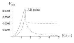
Figure 1: Global structure of vacuum. Solid and dashed curves show the evolutions of the potential energies at the monopole and left(right) dyon points for $0\leq{\rm Re}(a_{1})<\Lambda/(2\sqrt{2})$. The potential energies at the right dyon(dotted) and quark(dash-dotted) points for ${\rm Re}(a_{1})>\Lambda/(2\sqrt{2})$ are also plotted. We have fixed $\Lambda=2\sqrt{2}$.

As a result, we found the global SUSY minima at $a_{1}=0$ in the degenerated dyon and monopole singular points.

Next, let us turn on $\mu_{1}$ and $\lambda$. In the presence of the soft term, the gauge dynamics favors the monopole and the dyon points at $a_{1}=0$ as SUSY vacua besides the runaway vacua. It implies that if we add $\mu_{1}\not=0,\lambda\not=0$ terms which produce a vacuum at a point different from $a_{1}=0$ at the classical level, SUSY is dynamically broken as a consequence of the discrepancy of SUSY conditions between the classical and the quantum theories. Actually, turning on the mass $\mu_{1}$ and the FI parameter $\lambda$ realizes such a situation. In this case, the classical vacuum is at $a_{1}=-\lambda/\mu_{1}$, different from the point $a_{1}=0$ which the dynamics favors. A resultant SUSY breaking vacuum is realized at non-zero value of $a_{1}$. This is very similar to the SUSY breaking mechanism discussed in the Izawa-Yanagida-Intriligator-Thomas model in ${\cal N}=1$ SUSY gauge theory IzYa ; InTh . We show a schematic picture of our situation in Fig. 2.

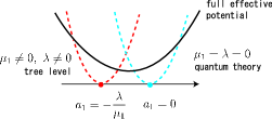
Figure 2: Schematic picture of SUSY breaking mechanism

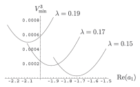
Figure 3: Local SUSY breaking minimum at the monopole singular point for $\mu_{1}=\mu_{2}=0.1$ and $\lambda=0.15,0.17,0.19$ from bottom to top. Here $0\leq\mathrm{Re}(a_{1})<\Lambda/2\sqrt{2}$.

Let us see in detail how this works for non-zero values of $\mu_{1},\mu_{2}$ and $\lambda$. Fig. 3 shows the evolution of the potential energies at the monopole point $V_{\mathrm{min}}^{3}$ for several values of $\lambda$ as a function of ${\rm Re}(a_{1})$ with $\mu_{1}=\mu_{2}=0.1$. The potential minimum is no longer realized at $a_{1}=0$, but the location is shifted to negative values of ${\rm Re}(a_{1})$ as is expected from the discussion in the previous paragraph. Furthermore, the potential energy has a non-zero value and therefore SUSY is dynamically broken. We find that the potential energies at the left and right dyon singular points also have the same structure. A qualitative picture of the evolutions of the potential minima is depicted in Fig. 4.

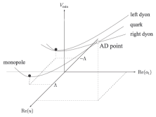
Figure 4: Qualitative picture of the evolutions of the potential minima.

In addition to these local minima, there are supersymmetric vacua on the Higgs branch which survive from the quantum corrections. We estimated the decay rate from our local minima to the SUSY vacua on the Higgs branch and found that the decay rate can be taken to be very small. This means our local minima are nothing but meta-stable SUSY breaking vacua.

References

• (1) K.ย Intriligator, N.ย Seiberg and D.ย Shih, JHEP 0604 (2006) 021 [arXiv:hep-th/0602239].
• (2) H.ย Ooguri, Y.ย Ookouchi and C.ย S.ย Park, arXiv:0704.3613 [hep-th].
• (3) J.ย Marsano, H.ย Ooguri, Y.ย Ookouchi and C.ย S.ย Park, Nucl.ย Phys.ย  B 798 (2008) 17 [arXiv:0712.3305 [hep-th]].
• (4) G.ย Pastras, arXiv:0705.0505 [hep-th].
• (5) M.ย Arai, C.ย Montonen, N.ย Okada and S.ย Sasaki, Phys.ย Rev.ย  D 76 (2007) 125009 [arXiv:0708.0668 [hep-th]].
• (6) M.ย Arai, C.ย Montonen, N.ย Okada and S.ย Sasaki, JHEP 0803 (2008) 004 [arXiv:0712.4252 [hep-th]].
• (7) N.ย Seiberg and E.ย Witten, Nucl.ย Phys.ย B 431 (1994) 484 [arXiv:hep-th/9408099].
• (8) K.ย I.ย Izawa and T.ย Yanagida, Prog.ย Theor.ย Phys.ย  95 (1996) 829 [arXiv:hep-th/9602180].
• (9) K.ย A.ย Intriligator and S.ย D.ย Thomas, Nucl.ย Phys.ย  B 473 (1996) 121 [arXiv:hep-th/9603158].