Abstract

The pressure, and the energy and entropy densities are determined for the $SU(3)$ gauge theory in $2+1$ dimensions from lattice Monte Carlo calculations in the interval $0.6\leq T/T_{c}\leq 15$. The finite temperature lattices simulated have temporal extent $N_{\tau}=2,4,6$ and 8, and spatial volumes $N_{S}^{2}$ such that the aspect ratio is $N_{S}/N_{\tau}=8$. To obtain the thermodynamical quantities, we calculate the averages of the temporal plaquettes $P_{\tau}$ and the spatial plaquettes $P_{S}$ on these lattices. We also need the zero temperature averages of the plaquettes $P_{0}$, calculated on symmetric lattices with $N_{\tau}=N_{S}$. We discuss in detail the finite size ($N_{S}$-dependent) effects. These disappear exponentially. For the zero temperature lattices we find that the coefficient of $N_{S}$ in the exponent is of the order of the glueball mass. On the finite temperature lattices it lies between the two lowest screening masses. For the aspect ratio equal to eight, the systematic errors coming from the finite size effects are much smaller than our statistical errors. We argue that in the continuum limit, at high enough temperature, the pressure can be parametrized by the very simple formula $p=T^{3}(a-b\,T_{c}/T)$ where $a$ and $b$ are two constants. Using the thermodynamical identities for a large homogeneous system, this parametrization then determines the other thermodynamical variables in the same temperature range.

1 Introduction

The determination of the thermodynamical variables in the high temperature phase of QCD is one of the main goals of lattice gauge theory. The values of those variables are of particular importance for the analysis of the data from high energy heavy ion collisions. Furthermore, the calculation of the free energy by straightforward perturbation theory is infrared divergent already at three loops. This divergence, which is connected to the electric screening mass, can be resummed, but at four loops new infrared divergences connected to the magnetic screening appear, which cannot be easily resummed. One may use dimensional reduction [1, 2, 3, 4], but the calculation of the free energy in this framework is a formidable task, which is not yet completely finished [5, 6, 7]. Therefore, at present a non perturbative theoretical method like lattice gauge theory is the only possibility to get quantitative results. This is particularly necessary below about twice the critical temperature, where perturbation theory even improved with dimensional reduction is not expected to work.

The numerical demand of lattice QCD with fermions makes it difficult to make a continuum extrapolation with controlled systematical errors. For improved staggered fermions, however, there exist new data for the timelike lattice spacings $N_{\tau}=4,6,8$ [8, 9]. In pure SU(3) gauge theory a continuum extrapolation has been performed a long time ago, but only up to $T=4T_{c}$[10]. In order to make contact with the different proposals for resummed perturbation theory, it would be very interesting to go to higher temperature. There are some recent results on this for $N_{\tau}=4$ with the Symanzik improved action [11].

In this article we study a closely related theory, namely pure SU(3) gauge theory in $2+1$ dimensions. This theory has many properties in common with $SU(3)$ gauge theory in $3+1$ dimensions. It has linear confinement and a deconfining phase transition at finite temperature. The infrared divergences in perturbation theory are stronger so that even the lowest non trivial order for the free energy is not calculable in straightforward perturbation theory[12].

We determine the thermodynamical variables and the equation of state by lattice Monte Carlo computations on several lattices. In our calculations we use the so called integral method [10, 13]. In order to change from the lattice coupling constant $\beta$ to the temperature $T$, we use a scaling function derived from values for the string tension $\sigma$ at zero temperature [14, 15, 16, 17]. Using the values for the critical couplings from Ref.[14], we may also express the above thermodynamical variables as functions of $T/T_{c}$. The method then gives directly the normalized trace of the energy momentum tensor, $(\epsilon-2p)/T^{3}$ as a function of $T/T_{c}$, where $\epsilon$ is the energy density and $p$ the pressure. Thermodynamical identities in a sufficiently large and homogeneous system means that the normalized pressure, $p/T^{3}$ can be derived directly from the trace through integration over $T$. From these two quantities further thermodynamical variables, like the energy density $\epsilon$ and the entropy density $s$ can be easily calculated. We determine the thermodynamical variables in the range $0.6\leq T/T_{c}\leq 15$, which in this theory means that the effective dimensionless coupling constant $g^{2}/T$ varies in the interval $3\geq g^{2}/T\geq 0.12$.

In Section 2 we present the problem and our adaptation of the integral method. In Section 3 we derive the $\beta$-function and determine its parameters. In Section 4 we present the results of our Monte Carlo calculation, and show that finite spatial lattice size effects are not present in the data. In Section 5 we discuss the results. Section 6, finally, is devoted to the conclusions.

2 The method

In this section we will first recapitulate some well known facts about thermodynamics and lattice gauge theory in $2+1$ dimensions. This serves essentially to fix our definitions and notations. We then describe the method employed to extract the thermodynamical quantities from lattice data, following ref. [10, 13]

We start with the Euclidean Lagrangian in the continuum theory,

$${\cal L}_{E}({\mathbf{A}}_{\mu}(x))=\frac{1}{2g^{2}}tr({\mathbf{F}}_{\mu\nu}(x){\mathbf{F}}_{\mu\nu}(x)).$$ (1)

Here, $x=(x_{0},x_{1},x_{2})$ is a three dimensional Euclidean vector. The dynamical variables are the gauge fields ${\mathbf{A}}_{\mu}(x)$, which are hermitean traceless matrices belonging to the algebra of the SU(3) group and

$${\mathbf{F}}_{\mu\nu}(x)=\partial_{\mu}{\mathbf{A}}_{\nu}(x)-\partial_{\nu}{\mathbf{A}}_{\mu}(x)+i[{\mathbf{A}}_{\mu}(x),{\mathbf{A}}_{\nu}(x)].$$ (2)

Note that $g^{2}$ has the dimension of mass in three dimensions.

The thermodynamics of the corresponding quantum theory is derived from the partition function, which is formally expressed as

$$Z(T,V,g^{2})=\int{\cal D}{\mathbf{A}}_{\mu}(x)e^{-\int^{1/T}_{0}dx_{0}\,\int_{V}d^{2}x{\cal L}_{E}({\mathbf{A}}_{\mu}(x))},$$ (3)

where $T$ is the temperature and $V$ the spatial volume.

From the partition function $Z$ we get the free energy

$$F(T,V,g^{2})=-T\log Z.$$ (4)

In the following we will use the pressure $p$, and the volume densities of the free energy, the internal energy and the entropy, and denote those by $f$, $\epsilon$ and $s$ respectively. We will assume that we have a large homogeneous system, in which case

$$p(T,g^{2}) = -f(T,g^{2}),$$ (5)

$$\epsilon(T,g^{2}) = T^{2}\frac{\partial}{\partial{T}}(p/T),$$ (6)

$$s(T,g^{2}) = \frac{\partial p}{\partial T}=\frac{\epsilon+p}{T}.$$ (7)

It follows that in $2+1$ dimensions we further have for the trace of the energy momentum tensor $\epsilon-2p$,

$$\frac{\epsilon-2p}{T^{3}}=T\frac{\partial}{\partial T}\left(\frac{p}{T^{3}}\right).$$ (8)

In fact we can use the left hand side as the basic quantity, from which the other thermodynamical quantities can be obtained apart from an integration constant.

In $2\,+\,1$ dimensions and for $g^{2}=0$ (the free gauge theory), the temperature $T$ is the only scale in the system, and the dimensionless quantities

$$\frac{p}{T^{3}},\frac{\epsilon}{T^{3}},\frac{s}{T^{2}},$$ (9)

are pure numbers. Thus, in this case the energy momentum tensor is traceless and

$$\epsilon = 2p,$$ (10)

$$s = \frac{3p}{T}.$$ (11)

The pressure for eight free gluons in two spatial dimensions is easily calculated to be

$$\frac{p}{T^{3}}=8\frac{1}{2\pi}\zeta(3)=1.5305...\,.$$ (12)

In this article we consider the theory regularized on a finite lattice with lattice spacing $a$ and with $N_{\tau}$ points in the (inverse) temperature direction, defined as the 0 direction and $N_{S}^{2}$ points in the space directions $1,2$. We denote the link variables starting from the site $x$ in the positive directions by $U_{\mu}(x),\mu=0,1,2$ and use the standard Wilson action:

$$S_{W}(U_{\mu}(x)) = \sum_{P}S(U_{P}),$$ (13)

$$S(U_{P}) = \beta\left(1-\frac{1}{3}Re\,Tr\,U_{P}\right),$$ (14)

where $P$ denotes one of the $3N_{\tau}\times N_{S}^{2}$ plaquettes on the lattice and $U_{P}$ is the product of the $U$-matrices around the plaquette. One should not confuse the dimensionless coupling constant $\beta$ with the inverse temperature, which we will not use with that notation. Defining $U_{\mu}(x)$ in terms of $A_{\mu}(x)$ by

$$U_{\mu}(x)\equiv e^{i\int^{x+a\hat{\mu}}_{x}\,A_{\mu}(x^{\prime})dx^{\prime}}\cong e^{iaA_{\mu}(x)},$$ (15)

one obtains the original Lagrangian from the classical limit of the lattice Lagrangian,

$$\lim_{a\rightarrow 0}\frac{S(U_{P})}{a^{4}} = \frac{\beta}{12}TrF_{\mu\nu}(x)F_{\mu\nu}(x),$$ (16)

$$\lim_{a\rightarrow 0}\,a\beta = \frac{6}{g^{2}}.$$ (17)

Furthermore we define the temperature and the volume on the lattice by

$$\frac{1}{T} = aN_{\tau},$$ (18)

$$V = (aN_{S})^{2}.$$ (19)

To obtain the thermodynamical quantities we need to calculate the free energy on the lattice,

$$p\, = \,-f\,=\,\frac{T}{V}\log Z,$$ (20)

$$Z = \int\prod_{x,\mu}\,dU_{\mu}(x)e^{-S_{W}(U_{\mu}(x))}.$$ (21)

The partition function cannot be calculated directly by Monte Carlo methods. Here we use the integral approach of Refs. [10, 13]. Thus we first calculate the derivative of $\log Z$ with respect to the lattice coupling constant $\beta$ at fixed $N_{\tau}$ and $N_{S}$. It is given by

$$\frac{d\log Z}{d\beta}=-N_{\tau}N_{S}^{2}\left\langle P_{S}+2P_{\tau}\right\rangle.$$ (22)

The negative sign may look strange, but we have not yet subtracted the pressure at zero temperature. Note that we define the plaquette average value $\left\langle P\right\rangle$ as

$$\left\langle P\right\rangle=\left\langle 1-\frac{1}{3}Re\,Tr\,U_{P}\right\rangle$$ (23)

and $P_{S}$ (resp. $P_{\tau}$) denotes a plaquette in the $\{1,2\}$ (resp. $\{0,1\}$ or $\{0,2\}$) plane. Averages $\left\langle\ldots\right\rangle$ are taken with respect to the Wilson weight corresponding to given lattice parameters. The averages containing either $P_{\tau}$ or $P_{S}$ are always taken on the finite temperature lattices $N_{\tau}<N_{S}$ and $\left\langle P_{0}\right\rangle$ will always denote average on the zero temperature lattice $N_{\tau}=N_{S}$.

Eqs. (20, 22) defines $p$ up to a constant with respect to $\beta$, so that for some $\beta^{0}$ to be chosen below we find

$$a^{3}\,p(\beta,N_{\tau},N_{S})=-\int^{\beta}_{\beta^{0}}\,d\beta^{\prime}\left\langle P_{S}+2P_{\tau}\right\rangle_{\beta^{\prime}}+a^{3}\,p(\beta^{0},N_{\tau},N_{S}).$$ (24)

We next subtract from this expression its value for $N_{\tau}=N_{S}$, which for $N_{S}$ large enough constitutes its zero temperature limit, and thus consider the quantity

$$a^{3}\,\biggl{(}p(\beta,N_{\tau},N_{S})-p(\beta,N_{S},N_{S})\biggr{)}$$

$$= \,\int^{\beta}_{\beta^{0}}\,d\beta^{\prime}\Biggl{(}3\,\left\langle P_{0}\right\rangle_{\beta^{\prime}}\,-\,\left\langle P_{S}+2P_{\tau}\right\rangle_{\beta^{\prime}}\Biggr{)}$$ (25)

$$+ a^{3}\,\biggl{(}p(\beta^{0},N_{\tau},N_{S})-p(\beta^{0},N_{S},N_{S})\biggr{)}.$$

The last term in this substracted expression for the pressure is still unknown, but it can be made negligible by choosing $\beta^{0}$ in such a way that $N_{\tau}$ is sufficiently larger than the correlation length at that value of $\beta$. To this extent then $p(\beta^{0},N_{\tau},N_{S}$) is insensitive to the replacement of $N_{\tau}$ by $N_{S}$ and the constant vanishes. Under this condition for $\beta^{0}$, our numerical estimate of the thermal (i.e. zero temperature subtracted) part of the pressure, which we denote by the same symbol $p$, is

$$\frac{p(\beta,N_{\tau},N_{S})}{T^{3}}\,=\,N_{\tau}^{3}\,\int^{\beta}_{\beta^{0}}\,d\beta^{\prime}\Delta S(\beta^{\prime},N_{\tau},N_{S}),$$ (26)

where

$$\Delta S(\beta,N_{\tau},N_{S})=3\left\langle P_{0}\right\rangle_{\beta}\,-\,\left\langle P_{S}+2P_{\tau}\right\rangle_{\beta}.$$ (27)

The above expression for the pressure is evaluated from simulations performed on $N_{\tau}\times N_{S}^{2}$ lattices, with the aspect ratio $N_{S}/N_{\tau}\geq 8$. In section 4 we will show that for this minimum aspect ratio we are sufficiently close to the thermodynamic limit, i.e. that the finite size corrections are smaller than our statistical errors.

In order to obtain the pressure from (26) as a function of $T/T_{c}$, where $T_{c}$ is the critical temperature of the continuum theory, we still need to relate $T/T_{c}$ to $\beta$,

$$\beta=\beta(T/T_{c}),$$ (28)

which will be discussed in Section 3. Finally we choose $\beta^{0}=\beta(T/T_{c}=0.6)$, after checking from the measurements that $N_{\tau}^{3}$ times the integrand in (26) is negligibly small at this temperature. According to (8,26,28), the normalized trace of the energy momentum tensor is finally given by

$$\frac{\epsilon-2p}{T^{3}} = T\frac{\partial}{\partial T}\left(\frac{p}{T^{3}}\right)$$ (29)

$$= N_{\tau}^{3}\,\Delta S\left(\beta\bigl{(}\frac{T}{T_{c}}\bigr{)},N_{\tau},N_{S}\right)\,T\frac{d\beta}{dT}.$$

From Eqs. (7), (26) and (29) one obtains the expressions for the energy and entropy densities $\epsilon$ and $s$.

3 Physical Scales for the Temperature

We need to express the thermodynamical variables, provided by (26) and (29) from lattice simulations, as functions of the lattice temperature $T$ defined in (18). This temperature has to be measured at some scale related to the continuum theory. The continuum coupling $g^{2}$ is such a scale, but it is interesting to consider other quantities of the same dimension, and thus proportional to $g^{2}$, which have a direct physical interpretation. Here we will use $\sqrt{\sigma}$, the square root of the zero temperature string tension, and $T_{c}$, the critical temperature, both in the continuum theory.

In this section, we construct the corresponding scaling functions which, given $N_{S}$ and $N_{\tau}$, represent the change of variable from $\beta$ to $T/\sqrt{\sigma}$, $T/T_{c}$ or $T/g^{2}$. We start with the former, namely

$$\beta\,=\,\beta_{\sigma}(T/\sqrt{\sigma})\quad\text{and its inverse}\quad\frac{T}{\sqrt{\sigma}}\,=\,\beta_{\sigma}^{\{-1\}}(\beta).$$ (30)

Passing from one scale to the other is just a multiplicative numerical factor, $T_{c}/\sqrt{\sigma}$, which must be also computed.

In the literature, there exist mainly two sets of data for the quantity

$$F_{\sigma}(\beta)\,=\,a\,\sqrt{\sigma},$$ (31)

obtained from lattice simulations in various domains of $N_{S}$ and $\beta$. A large set $\beta\in[8:50]$, referred to as $A$ in what follows, has been covered in [15, 16], while recent simulations [17], provide high accuracy data at three $\beta$ values only, 14.717, 21 and 40 (set $B$). Both sets are included in table 1. How we use them is explained below.

$\beta$	$N_{s}$	$F_{\sigma}(\beta)=a\sqrt{\sigma}$	ref.
8.156	16	0.5677(19)	[15]
10	24	0.42443(70)	[15]
12	24	0.33679(21)	[15]
14	24	0.27885(13)	[15]
14.7172		0.26101(9)	[17]
15	24	0.2570(15)	[16]
18	32	0.20712(24)	[15]
19	32	0.19447(23)	[15]
21		0.173948(75)	[17]
22	32	0.16555(24)	[15]
24	32	0.15112(23)	[15]
28	32	0.1275(2)	[16]
34	40	0.10379(26)	[16]
40		0.087046(75)	[17]
50	48	0.07021(5)	[15]

Table 1: Data for the string tension. Each line gives the values of $\beta$, $N_{S}$, and $F_{\sigma}(\beta)\,=\,a\,\sqrt{\sigma}$, and the corresponding reference.

For any value of $\beta$ occuring in Table 1, using Eqs. (31,18) gives directly

$$\frac{T}{\sqrt{\sigma}}\,=\,\frac{1}{N_{\tau}\,F_{\sigma}(\beta)}.$$ (32)

However, we need in practice to evaluate $T/\sqrt{\sigma}(\beta)$ for a denser and larger set ($\beta\in[8:400]$) of $\beta$ values. This is required in particular to obtain the pressure from the integral (26), in a range of temperatures $T/T_{c}$ from about 0.6 to 15. This we achieve by making fits to the data of Table 1. We use the form

$$F_{\sigma}(\beta)=\frac{c_{1}}{\beta}+\frac{c_{2}}{\beta^{2}}+\frac{c_{3}}{\beta^{3}}.$$ (33)

This choice is done for the sole purpose of representing properly the data, with no theoretical prejudice about the actual behaviour of $F_{\sigma}$ around $1/\beta$=0. An investigation shows that there exists a systematic although small discrepancy between the sets $A$ and $B$, and we found it adequate to fit them separately rather than altogether. Replacing the symbol $c_{i}$ of (33) by $a_{i}$ and $b_{i}$ respectively for $A$ and $B$, the two fits give

$$a_{1}=3.37(1)\quad a_{2}=3.90(25)\quad a_{3}=50.1(1.8)$$ (34)

$$b_{1}=3.34(1)\quad b_{2}=4.68(50)\quad b_{3}=39.8(5.0).$$ (35)

The relative difference of $1\%$ between $a_{1}$ and $b_{1}$ gives the order of magnitude of the systematic effect due to choosing $A$ or $B$ at large $\beta$. At low $\beta$, one might worry that the large cubic term found in both cases casts a doubt on the validity of the extrapolations. We note however that table 1 gives $F_{\sigma}$ = 0.568(2) at $\beta=8.156$ [15], less than $3\%$ away from the average values 0.564 and 0.553 one gets respectively (with larger errors) from $A$ and $B$. Furthermore, as we shall see in the next sections, such low values of $\beta$ are used only for $N_{\tau}\,=\,2$, which plays a very marginal role in our main physical results. With that in mind and for definiteness, we will use the parameters (35) corresponding to the high precision data [17]. The numerical value of $T/\sqrt{\sigma}$ given $\beta,N_{\tau}$ is thus obtained by inserting (33) in (32) with $c_{i}=b_{i}$, $b_{i}$ as in (35). The errors on $\sqrt{\sigma}$ in the input data imply an error on this change of variable, to be estimated (see below).

Our last task before that is to define $T$ using the scale $T_{c}$, the critical temperature in the continuum, that is in the limit $N_{\tau}$ and $N_{S}\to\infty$. Since we already know $T/\sqrt{\sigma}$ we thus compute $T_{c}/\sqrt{\sigma}$. From (32), we write

$$\frac{T_{c}}{\sqrt{\sigma}}\,=\,\lim_{N_{\tau}\to\infty}\,\frac{1}{N_{\tau}\,F_{\sigma}[\beta_{c}(N_{\tau})]},$$ (36)

where $\beta_{c}(N_{\tau})$ is the critical lattice coupling determined by lattice simulations at given $N_{\tau}$. In this expression, the $N_{S}=\infty$ limit should have been taken first. As will be shown in section 4 on the basis of our simulations, the value of $N_{S}$ (8$\times N_{\tau}$) for each $N_{\tau}$ is large enough to eliminate any finite $N_{S}$ effect. In order to perform the limit (36), we use the set of $\beta_{c}$ obtained in [15] for $N_{\tau}$=2, 4 and 6, that is respectively $\beta_{c}$=8.155(15), 14.74(5), and 21.34(4)(11). More recent data on $\beta_{c}(N_{\tau})$ at $N_{\tau}=2,3,4,5$ can be found in [18] and they do not modify our estimate, which is:

$$\frac{T_{c}}{\sqrt{\sigma}}\,=\,1.00(4).$$ (37)

The ratio to this constant of $T/\sqrt{\sigma}$ is $T/T_{c}$, which will be used as the temperature variable in the rest of the paper.

The error in (37), as well as any other error quoted in the present and subsequent sections have been estimated using the so-called bootstrap method (see [19, 20]). To be concrete, we describe it in detail for this very typical case.

The set of initial data, noted $x_{j}$ for short, consists of values and errors for $a\,\sqrt{\sigma}$ and $\beta_{c}$ at given values of external variables $\beta$ or $N_{\tau}$. All $x_{j}$ are assumed to be independent and gaussians. We performed the following steps

Step 1: From the last assumption, generate another equivalent set of input variables $y_{j}$.

Step 2: Fit the coefficients $c_{i}$ of (33) to the $y_{j}$ values. (Note that in the case where $y_{j}$ represents the data of [17], the 3 coefficients $a_{i}$ are exactly determined by the 3 $y_{j}$. Standard $\chi^{2}$ methods would not give any estimate of their errors).

Step 3: Compute $F_{\sigma}(\beta)$ for $\beta\,=\,\beta_{c}(N_{\tau})$

Step 4: Fit a quadratic form in $1/N_{\tau}$ to the 3 values obtained for the inverse of $N_{\tau}\,F_{\sigma}(\beta_{c}(N_{\tau}))$. From Eq. (37), its value at $1/N_{\tau}$=0 is an estimate of $T_{c}/\sqrt{\sigma}$.

Step 5: Repeat everything from Step 1 many times (100), each time with a new set of $y_{j}$.

Our result (37) gives the value of $T_{c}/\sqrt{\sigma}$ for $y_{i}\,=\,x_{i}$, with an error equal to the standard deviation measured within the set of estimates obtained at Step 5.

A different way to determine a $\beta$ function of the form (30) is to use directly the knowledge of $\beta_{c}$ available for various $N_{\tau}$ values. We expand $\beta$ as a Laurent series in $a\,g^{2}$, writing

$$\beta\,=\,\frac{6}{a\,g^{2}}\,+\,b\,+\,c\,a\,g^{2}\,+\,\cdots.$$ (38)

The first term corresponds to the classical limit of the lattice action. We include as many terms as there are known $\beta_{c}$ values, and consider the truncated series obtained as representing the first terms of an asymptotic series. We then replace the lattice spacing $a$ by $1/(N_{\tau}\,T)$ and introduce the scale $T_{c}$ to rewrite (38) as

$$\frac{\beta}{N_{\tau}}\,=\,\frac{6\,T_{c}}{g^{2}}\,\frac{T}{T_{c}}\,+\,\frac{b}{N_{\tau}}\,+\,c\,\frac{g^{2}}{T_{c}}\,\frac{T_{c}}{T}\,\frac{1}{N_{\tau}^{2}}\,+\,\cdots.$$ (39)

This expansion now constitutes an expansion in $1/N_{\tau}$, whose $1/N_{\tau}\,=\,0$ limit gives an estimate of $T_{c}$ in units of $g^{2}$ in the continuum limit.

From Eq. (39) and the values of $\beta_{c}$ quoted in [15] for $N_{\tau}=$ 2, 4, 6, namely 8.149(3), 14.74(5), 21.34(11) respectively, one finds

$$\frac{T_{c}}{g^{2}}\,=\,0.55(2)\,;\quad\quad b=1.5(6)\,;\quad\quad c\,=\,0.06(50).$$ (40)

We observe that the $1/N_{\tau}^{2}$ term is compatible with zero in the range of interest, which means that the $\beta$ function in terms of $T/g^{2}$ is essentially linear. Although the $\beta$ functions determined via the knowledge of the string tension and via Eqs. (39, 40) need not be the same at finite $N_{\tau}$, we find them very close one to the other, so that they can be used equivalently in the present work. In practice, an accurate representation of our findings for the $\beta$-function, valid in the whole range explored in $\beta$ and $N_{\tau}$ is

$$\frac{\beta}{N_{\tau}}=3.3\,\frac{T}{T_{c}}\,+\,\frac{1.5}{N_{\tau}}.$$ (41)

This formula is useful in order to jump easily from functions of $\beta$ to functions of $T/T_{c}$. Only when precise estimates of errors in final results is needed is it necessary to go through the process described above and apply the bootstrap method.

4 Results of the Simulations

The results of our simulations consist of high precision plaquette data, that is their average values and statistical errors, for zero and finite temperature lattices. These data are shown in the appendix Here we present and discuss the quantity $N_{\tau}^{3}\,\Delta S\,=\,N_{\tau}^{3}\,(3\left\langle P_{0}\right\rangle\,-\,\left\langle 2P_{\tau}+P_{S}\right\rangle)$ which was shown in section 2 to constitute the basis for all computations of the thermodynamical variables.

An important source of possible systematic errors for the quantities of physical interest resides in the finite size effects (FSE) at $\beta$ and $N_{\tau}$ fixed due to $N_{S}$ being finite. A reason for this is that although $\left\langle\operatorname{T}r{U_{P}}\right\rangle\,/\,3$ is of order one, very strong cancellations occur in $N_{\tau}^{3}\,\Delta S$. According to the definitions in section 2, $\left\langle P\right\rangle$ is expected to go to 0 as $\beta\to\infty$. Although its precise behaviour around $\beta^{-1}\,=\,0$ is unknown, we assume that it can be numerically represented by a (probably asymptotic) series in $\beta^{-1}$. We find that the linear term is absent and that $N_{\tau}^{3}\,\Delta S$ is of the form

$$N_{\tau}^{3}\,\Delta S\,\approx\,\frac{A}{\beta^{2}}+O(\beta^{-3}),$$ (42)

at large $\beta$, with $A$ a function of $N_{\tau}$ and $N_{S}$. This behaviour was verified to a high degree of precision from our data.

We, of course, have to make sure that the finite size effects occuring in the distinct measurements of $P_{0},P_{\tau},P_{S}$ are so small that the corresponding effects in $N_{\tau}^{3}\,\Delta S$ lead to acceptable errors, smaller than the statistical ones. These finite size effects should be related to the largest gauge invariant correlation length of the system, a priori different for $P_{0}$, and for $P_{S}$ and $P_{\tau}$. In the former case we are in the confined phase at $T=0$, where the largest correlation length is given by the inverse of the lowest glueball mass, whose measurement was reported in [16]. In the latter case, it is given by the screening length, measured in [21].

Here we report the results of a systematic study of the FSE observed in $P_{0},P_{\tau},P_{S}$, from simulations performed, at $N_{\tau}$=4 fixed, for a large set [15:150] of $\beta$ values and $N_{S}\in[6:48]$.

Each $\left\langle P\right\rangle$ at a given $\beta$ was analyzed as a function of $N_{S}$, and parametrized as

$$\left\langle P\right\rangle_{\beta,N_{S}}\,=\,A(\beta)\,-\,B(\beta)\,\exp(-\mu(\beta)\,N_{S}).$$ (43)

For a lattice spacing $a$, this corresponds to the assumption that an effective correlation length

$$\xi(\beta)\,=\,a/\mu(\beta)$$ (44)

leads to FSE which decay exponentially in the ratio $L/\xi$, where $L\,=\,a\,N_{S}$ is the spatial extent of the lattice. By fitting Eq. (43) to the data, we determined $A(\beta)$, the plaquette value on a spatially infinite lattice, the weight $B(\beta)$ of the exponential component, and the effective mass $\mu(\beta)$ in lattice units. Depending on the type of plaquette considered, the quantities $A,B,\mu$ are given the corresponding subscript $0$ or $\tau$ or $S$.

The general features of our findings on these FSE are the followings.

1. The parametrization (43) is always adequate. As an illustration, Fig. (1) shows how the data for $\left\langle P_{S}(\beta,N_{S})\right\rangle$ approach their $N_{S}=\infty$ limit, together with fits to Eq. (43).

   

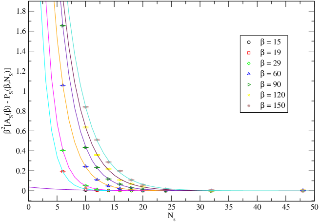
   Figure 1: The average spatial plaquette $\left\langle P_{S}(\beta,N_{S})\right\rangle$ approaches its limit $\left\langle P_{S}(\beta,\infty)\right\rangle$ from below, exponentially in $N_{S}$. For clarity of the figure, the quantity $A_{S}(\beta)\,-\,\left\langle P_{S}(\beta,N_{S})\right\rangle$ has been multiplied by $\beta^{2}$.

2. Close to $\beta_{c}$, the $B$ coefficients are of opposite signs in $P_{\tau}$ and $P_{S}$, and a partial cancellation of the FSE occurs. They are of the same positive sign in $P_{0}$ and $P_{S}$, which again lowers the overall FSE.

3. The mass parameter $\mu_{\tau}$, found to be around .45 for $\beta/N_{\tau}$ large is poorly determined. On the contrary, $\mu_{S}$ is well determined, and it lies in between the two screening masses $M_{S}$ and $M_{P}$ found in [21], as illustrated in Fig. (2). In the range $\beta\in[15:34]$ for which data on glueball masses exist [16], we find that $\mu_{0}$ is lower than those, but only by about $20\%$. In the whole range $\beta\in[15:150]$ we have approximate scaling, i.e. $\beta\,\mu_{0}(\beta)\propto\mu_{0}(\beta)/a$ is nearly constant.

4. Finally the comparison with the statistical errors of the effects due to $N_{S}$ finite shows that the latter can be neglected in our final measurements, all performed with the aspect ratio $\xi=N_{S}/N_{\tau}=8$. In the present exploration, we may compare the cases $\xi=4$ and $\xi=8$ corresponding respectively to $N_{S}$=16 and 32. Then for each $\left\langle P\right\rangle$, the $N_{S}-$dependent term in (43) is reduced by a factor $\exp(16\,\mu)$ if $\xi=8$, that is at least by two orders of magnitude in typical cases. Moreover,as mentioned in point 2 above, the contributions of these terms to $N_{\tau}^{3}\,\Delta S$ from different plaquettes tend to cancel each other. On the contrary the statistical errors are much larger in $N_{\tau}^{3}\,\Delta S$ than in $\left\langle P\right\rangle$ in relative value.

   

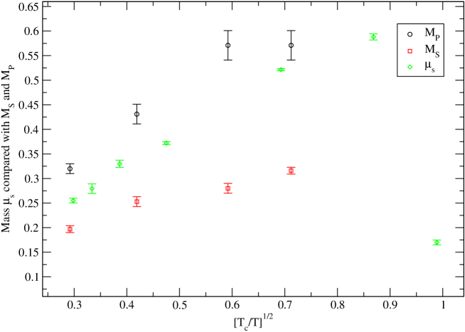
   Figure 2:

   Comparison of the inverse correlation length $\mu_{S}$ appearing in the FSE for $P_{S}$ with the screening masses $M_{S}$ and $M_{P}$ determined in Ref.[21].

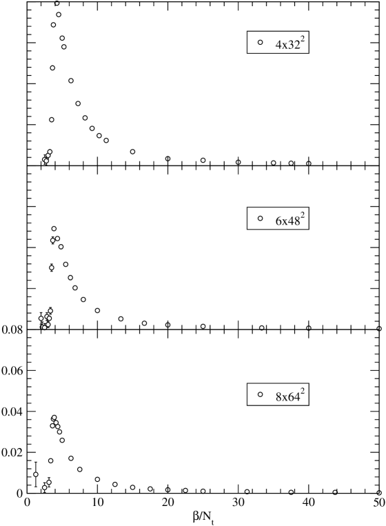
The results for $N_{\tau}^{3}\,\Delta S$, for those lattice sizes of particular interest in the final computation of the thermodynamical variables ($N_{\tau}=4,6,8$) are presented in figure 3. Their numerical values are given in the tables of the appendix, where the case $N_{\tau}=2$ is also included.

Figure 3: The average plaquette combination $N_{\tau}^{3}\Delta S$ for $N_{\tau}=4,6,8$. Their values and errors (in most cases smaller than the point sizes) are tabulated in the appendix. On each plot the horizontal scale is $\beta\,/\,N_{\tau}$ for easier comparison. The vertical scale is the same on all plots.

5 Thermodynamics

From the results presented, just above for $N_{\tau}^{3}\,\Delta S$ as a function of the lattice coupling $\beta$ and in section 3 for the scaling function relating $\beta$ to the temperature, the three thermodynamical variables $\epsilon,\,p$ and $s$ can be explicitly determined from the formulae of section 2.

For definitness, we choose to measure the temperature in units of the critical temperature. The temperature variable and the scaling function are then denoted

$$t\, = \,\frac{T}{T_{c}},$$ (45)

$$\beta\, = \,\beta(t).$$ (46)

On a given $N_{\tau}\,\times\,N_{S}^{2}$ lattice, the dimensionless energy and pressure densities $\epsilon/T^{3}$ and $p/T^{3}$ follow from Eqs. (26, 29) rewritten as

$$\frac{\epsilon-2p}{T^{3}}(t) = N_{\tau}^{3}\,\Delta S\,\biggl{(}\beta(t)\biggr{)}\,t\frac{d\beta}{dt},$$ (47)

$$\frac{p(t)}{T^{3}}\, = \,N_{\tau}^{3}\,\int^{\beta(t)}_{\beta(t_{0})}\,d\beta^{\prime}\Delta S(\beta^{\prime}).$$ (48)

In this integral, we choose $t_{0}\,=\,0.6$, a temperature below which the integrand is always negligible. From these equations one directly obtains $p/T^{3}$ and $\epsilon/T^{3}$; the entropy density $s/T^{2}$ follows from (7).

In order to use Eqs. (47) in practice, and in particular to perform the integral defining the pressure conveniently, we have interpolated $N_{\tau}^{3}\,\Delta S(\beta(t))$ via a smooth function $f(t)$. In the absence of any theoretical ansatz for the shape observed in figure 3, we choose the simplest parametrization adapted to the description of a sharp rise in the vicinity of the critical point $t$=1, and the $t^{-2}$ fall off at large t expected from Eqs.(42,41). The following function constitutes an accurate representation of $N_{\tau}^{3}\,\Delta S(\beta(t))$ within errors

$$f(t)=\frac{a_{1}t^{2}}{1+a_{2}t^{4}}\frac{1+a_{3}\,e^{a_{5}(t-1)}}{1+a_{4}\,e^{a_{5}(t-1)}}.$$ (49)

Figure 4: Trace of the energy momentum tensor.

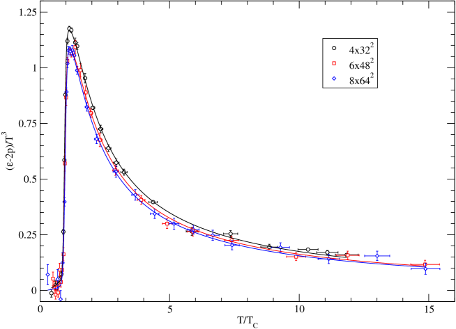
The adequacy of this function for our purposes is illustrated by the curves drawn through the data points in figure 4. The horizontal error bars represent the errors in the change of variable $\beta\,\to\,t=T/T_{c}$ described in section 3. They are of the order of 3 percents of $t$.

One may worry that choosing a specific function like (49) introduces a systematic error into subsequent calculations. A different choice was tried during this investigation. To the extent that it provided a comparable agreement with the data to which it was fitted, it leads, for example for the pressure, to differences much smaller than the statistical errors. However one must keep in mind that although $f(t)$ constitutes a good interpolation of the data within errors, the systematic errors attached to its use above $t\approx 15$ are not controlled.

Figure 5: The pressure measured on lattices with $N_{\tau}\,=\,2,4,6,8$ and $N_{S}\,=\,8\,N_{\tau}$

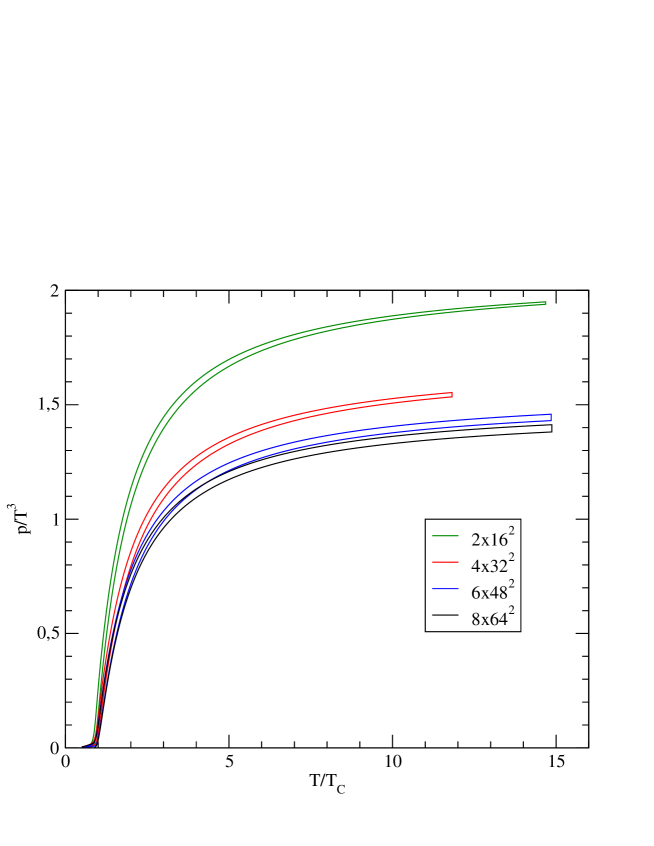
Our final results for the pressure at $N_{\tau}\,=\,2,4,6,8$ with $N_{S}\,=\,8\,N_{\tau}$ are shown in figure 5. The errors on the scale $t$, which we showed in figure 4, do not affect the pressure, which varies slowly where they become important (at large $t$). For the largest lattice considered ($N_{\tau}\,=\,8$), figure 6 compares the three thermodynamical variables, after multiplication by coefficients such that they would be the same in the free theory (see Eq. 10). The continuum Stefan-Boltzmann value for a free gas (horizontal dotted line) is also shown.

All the errors on the quantities plotted in figures 4, 5 and 6 have been estimated using the bootstrap method, similarly to the case described in section 3 for the calculation of $T/\sqrt{\sigma}$.

Figure 6: The pressure, and the energy and entropy densities for the largest lattice size ($8\text{x}64^{2}$).

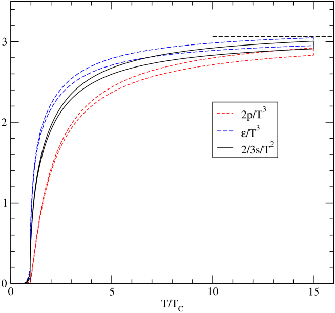
Let us now comment these results, whose extensions towards the continuum limit $1/N_{\tau}\,=\,0$ and to larger temperatures are highly desirable. A look at the results suggests that the continuum limit is nearly reached at $N_{\tau}=8$, the more so $t$ is large. We observe that the values of $(\epsilon-2p)/T^{3}$, at least above $t\approx 5$ hardly distinguish between $N_{\tau}\,=\,6$ and 8, and that the difference between the corresponding pressures does not exceed $\approx 2\sigma$. More quantitative statements however are hard to produce. Attempts at fitting quadratic functions in $1/N_{\tau}$ or $1/N_{\tau}^{2}$ to the pressure at fixed $t$ remained inconclusive, with no strong constraint on the continuum limit.

We then turn to the question of the high temperature behaviour. We already noticed (42) that the tail at large $\beta$ of $N_{\tau}^{3}\,\Delta S$ was compatible with $1/\beta^{2}$, which implies via (41)

$$\frac{\epsilon-2p}{T^{3}}\approx\frac{b}{t};\quad t>t_{1}.$$ (50)

for some large enough $t_{1}$. Since this appears to be true for any $N_{\tau}$, it is reasonable to expect that it is also valid in the continuum. We thus formulate the following ansatz: For $t$ larger than some $t_{min}$, the continuum limit of $(\epsilon-2p)/T^{3}$ is close to its value measured at $N_{\tau}\,=\,8$ and it can be parametrized there by $b/t$. We then obtain from Eqs. (47, 41)

$t_{min}$	$b$	$p/T^{3}(t_{min})$	$p/T^{3}(\infty)$
4.0	1.81(7)	1.13(2)	1.58
6.0	1.7(1)	1.27(2)	1.56
8.0	1.6(2)	1.34(2)	1.53

Table 2:

$$\frac{p}{T^{3}}(t) = \int_{t_{0}}^{t}\text{d}t\frac{1}{t}\frac{\epsilon-2p}{T^{3}}(t),$$ (51)

$$= a\,-\,\frac{b}{t},$$ (52)

$$a = \frac{p}{T^{3}}(t_{min})\,+\,\frac{b}{t_{min}}.$$ (53)

For $N_{\tau}=8$, the data between $t\approx 4$ and $t=15$ (the largest value explored) is compatible with a behaviour of the type (50). Suppose now that this remains true above $t$=15. Then from (52,53), we have

$$\frac{p}{T^{3}}(t=\infty)\,=\,\frac{p}{T^{3}}(t_{min})\,+\,\frac{b}{t_{min}}.$$ (54)

Given $t_{min}$, we get $b$ from $(\epsilon-2p)/T^{3}(t_{min})$, and $p/T^{3}(t_{min})$ is known from (51), so that a consistency check is that $p/T^{3}(t=\infty)$ is independent of $t_{min}$. In table  2, we report the values found for $b$ and $p/T^{3}(t=\infty)$ for $t_{min}$ = 4,6 and 8. We did not try to estimate any error on $p/T^{3}(t=\infty)$, certainly affected by uncontrolled systematics. Its value is stable with respect to $t_{min}$, and although it is obtained for $N_{\tau}$ finite, it is found close to the continuum Stefan-Boltzmann value for a free gas, 1.53.

6 Conclusions

In this article we have determined the thermodynamical quantities for SU(3) gauge theory in two spatial dimensions. This determination has been performed through lattice simulations, measuring the thermodynamical variables as functions of the lattice coupling $\beta$. We then constructed the scaling function connecting $\beta$ to the temperature expressed in units of various physical quantities, the square root $\sqrt{\sigma}$ of the zero temperature string tension, the coupling constant $g^{2}$ of the continuum theory and the critical temperature $T_{c}$. In particular, we determined the ratios $T_{c}/\sqrt{\sigma}$ and $T_{c}/g^{2}$ to be respectively 1.00(4) and 0.55(2). This construction has been discussed in detail, using published data on the string tension and on the critical lattice coupling $\beta_{c}$ .We finally kept $T_{c}$ as the temperature scale and presented the thermodynamical variables as functions of $T/T_{c}$.

We have determined the finite volume $N_{S}$ effects at fixed bare coupling constant $\beta$ by a careful analysis and shown that they are negligible compared to the statistical errors. We have further shown that those finite size effects fall off exponentially with $N_{S}$, and that the coefficient in the exponent multiplying $N_{S}$ is consistent within about $20\%$ with the longest correlation lengths expected on the various lattices, namely the inverse of the lowest glue ball mass on the zero temperature lattices, and the lowest screening length on the finite temperature lattices. This has lead us to choose the aspect ratio $N_{S}/N_{\tau}=8$, for which the finite size effects are much smaller then the statistical errors.

We investigated the finite lattice spacing effects by simulating lattices with extension in the temperature direction $N_{\tau}=2,4,6,8$. We found that $N_{\tau}=8$ is large enough to be near to the continuum limit. We have not presented attempts to extrapolate the thermodynamical variables to the continuum, because additional systematic errors appear. Instead we have analyzed the thermodynamical variables for $N_{\tau}=8$. We find that for large enough temperatures, well above the phase transition region, the pressure can be represented by a very simple function, namely $p=T^{3}\,(a-bT_{c}/T)$. Using the thermodynamical identities for a large homogeneous system we obtain the corresponding formulae for the other thermodynamical quantities.

Improving our findings in view of a quantitative determination of the continuum limit requires a more precise analysis of the $N_{\tau}$ dependence of the basic quantity $N_{\tau}^{3}\,\Delta S$. Larger statistics and/or larger lattices are possible ways in this direction.

7 Acknowledgements

This work is supported through by the European Community’s Sixth Framework Programme, network contracts MRTN-CT-2004-005616(ENRAGE) and CT-2004-517186(COCOS) and KBN grant 1P03B-04029. We thank the IPhT (CEA-Saclay) and the Institute of Physics at the Jagiellonian University ( Krakow) for their kind hospitality. Furthermore B.P. is grateful for the hospitality of the TIFR, Mumbai and for discussions with R. Gavai and Sourendu Gupta. P.B. thanks Fakultät für a Physik (University of Bielefeld) for kind hospitality and for discussions with O. Kaczmarek and E. Laermann.

Appendix A Data

The data were produced from a standard $SU(3)$ MC program. We used a mixture of heatbath and overrelaxation moves, with typically one heatbath sweep after 2 to 4 overrelaxation sweeps. All the simulations were done on the COCOS opteron cluster in the Institute of Physics, Jagiellonian University. This appendix presents the data for the plaquette averages $\left\langle P_{x}\right\rangle=1-\frac{1}{3}\operatorname{T}r\left\langle U_{P_{x}}\right\rangle$. The subscripts $S$ and $\tau$ denote spacelike and timelike plaquettes respectively, on finite temperature lattices ($N_{\tau}<N_{S}$). The subscript zero denotes plaquettes on zero temperature lattices ($N_{\tau}=N_{S}$). For each of the $N_{\tau}\,\times\,N_{S}^{2}$ or $N_{S}^{3}$ lattices, as functions of $\beta$ we list the values of $\left\langle P_{\tau}\right\rangle$, $\left\langle P_{S}\right\rangle$, $\left\langle P_{0}\right\rangle$, and $\left\langle N_{\tau}^{3}\Delta S\right\rangle$ from which the thermodynamical variables are finally computed. The errors were estimated using standard methods. We took care of strong correlations between $P_{\tau}$ and $P_{S}$, by first measuring the statistical errors for the combination $2P_{\tau}\,+\,P_{S}$, and adding them quadratically to those of the independent quantity 3$P_{0}$ to finally get the errors on $\left\langle\Delta S\right\rangle\,=\,\left\langle 3P_{0}-(2P_{\tau}\,+\,P_{S})\right\rangle$

$\beta$	$\left\langle P_{\tau}\right\rangle$	$\left\langle P_{S}\right\rangle$	$\left\langle P_{0}\right\rangle$	$\left\langle N_{\tau}^{3}\,\Delta S\right\rangle$
$4.00$	$0.715487(18)$	$0.715548(24)$	$0.715527(11)$	$0.00048(45)$
$6.00$	$0.541947(21)$	$0.542644(25)$	$0.542474(14)$	$0.00709(57)$
$6.50$	$0.498643(22)$	$0.499733(24)$	$0.499415(14)$	$0.00981(58)$
$7.00$	$0.457750(21)$	$0.459285(23)$	$0.458821(14)$	$0.01342(57)$
$7.50$	$0.420260(21)$	$0.422586(22)$	$0.422054(13)$	$0.02446(55)$
$8.00$	$0.382967(42)$	$0.389985(20)$	$0.3896419(97)$	$0.10405(77)$
$8.50$	$0.346390(21)$	$0.362726(18)$	$0.361541(11)$	$0.23293(49)$
$9.00$	$0.321171(16)$	$0.340272(16)$	$0.3372283(98)$	$0.23257(41)$
$9.50$	$0.300423(14)$	$0.320794(16)$	$0.3160913(90)$	$0.21306(36)$
$10.00$	$0.282596(13)$	$0.303523(15)$	$0.2975888(48)$	$0.19242(29)$
$11.00$	$0.253093(11)$	$0.274289(13)$	$0.2666359(42)$	$0.15545(25)$
$13.00$	$0.2100280(87)$	$0.230317(11)$	$0.2211848(33)$	$0.10545(20)$
$14.00$	$0.1936981(79)$	$0.213253(10)$	$0.2039362(31)$	$0.08928(19)$
$15.00$	$0.1797770(73)$	$0.1986216(94)$	$0.1892295(28)$	$0.07610(17)$
$16.00$	$0.1677617(67)$	$0.1858851(87)$	$0.1765258(26)$	$0.06535(16)$
$17.00$	$0.1572549(63)$	$0.1746807(82)$	$0.1654467(24)$	$0.05720(15)$
$18.00$	$0.1479903(59)$	$0.1647495(78)$	$0.1556880(22)$	$0.05067(14)$
$20.00$	$0.1324407(53)$	$0.1479638(70)$	$0.1392945(20)$	$0.04031(12)$
$21.00$	$0.1258401(49)$	$0.1407836(66)$	$0.1323299(19)$	$0.03621(12)$
$25.00$	$0.1049274(41)$	$0.1179602(56)$	$0.1103147(16)$	$0.025033(96)$
$29.00$	$0.0900011(35)$	$0.1015174(48)$	$0.0945963(13)$	$0.018155(82)$
$33.00$	$0.0788007(31)$	$0.0891024(42)$	$0.0828101(12)$	$0.013813(72)$
$37.00$	$0.0700760(27)$	$0.0793988(38)$	$0.0736427(10)$	$0.011019(64)$
$41.00$	$0.0631038(24)$	$0.0716004(34)$	$0.06630419(53)$	$0.008836(54)$
$45.00$	$0.0573848(22)$	$0.0652062(31)$	$0.06029866(84)$	$0.007362(52)$
$60.00$	$0.0428417(16)$	$0.0488355(23)$	$0.04501735(62)$	$0.004265(39)$
$80.00$	$0.0320233(12)$	$0.0365998(17)$	$0.03364921(47)$	$0.002410(29)$
$100.00$	$0.02556863(98)$	$0.0292673(14)$	$0.02686572(37)$	$0.001541(23)$
$120.00$	$0.02127680(81)$	$0.0243810(12)$	$0.02235950(44)$	$0.001152(21)$
$200.00$	$0.01273399(49)$	$0.01462132(70)$	$0.01338190(26)$	$0.000451(12)$

Table 3: Plaquette data for lattices of size $2\text{x}16^{2}$ and $16^{3}$.

Table 4: Plaquette data for lattices of size $4\text{x}32^{2}$ and $32^{3}$.

Table 5: Plaquette data for lattices of size $6\text{x}48^{2}$ and $48^{3}$.

Table 6: Plaquette data for lattices of size $8\text{x}64^{2}$ and $64^{3}$.

References

- [1] P. Ginsparg, Nucl. Phys. B170(1980)388.
- [2] T. Appelquist and R. Pisarski, Phys. Rev. D23(1981)2350.
- [3] T. Reisz, Z. Phys. C53(1992)169.
- [4] L. Kärkäinen, P. Lacock, B. Petersson and T. Reisz, Phys. Lett. 282B(1992)121, Nucl. Phys. B395(1993)733.
- [5] E. Braaten and A. Nieto, Phys. Rev. D53(1996)3421, [hep-ph/9510408].
- [6] K. Kajantie, M. Laine, K. Rummukainen and Y. Schröder, Phys. Rev. Lett. 86(2001)10, [hep-ph/0007109].
- [7] C. Torrero, M. Laine, Y. Schroder, F. DiRenzo and V. Miccio, [arXiv:0711.1176].
- [8] M. Cheng et.al., Phys. Rev. D77 (2008) 014511.
- [9] F. Karsch, to appear in the proceedings of Quark Matter 2008: 20th International Conference on Ultra-Relativistic Nucleus Nucleus Collisions (QM2008), Jaipur, India, 4-10 February 2008, [arXiv:0804.4148].
- [10] G. Boyd, J. Engels, F. Karsch, E. Laermann, C. Legeland, M. Luetgemeier and B. Petersson, Nucl. Phys. B469(1996)419, [hep-lat/9602007].
- [11] G. Endrodi, Z. Fodor, S. D. Katz and K. K. Szabo, PoS LATTICE2007, 228,2006. [arXiv:0710.4197]
- [12] E. D’Hoker, Nucl. Phys. B201(1982)401.
- [13] J. Engels, J. Fingberg, F. Karsch, D. Miller and M. Weber, Phys. Lett. B252(1990)625.
- [14] J.Engels, F. Karsch, E. Laermann, C. Legeland, M. Lütgemeier, B. Petersson, T. Scheideler, Nucl. Phys. Proc. Suppl. 53(1997)420, [hep-lat/9608099].
- [15] C. Legeland, Thesis, Bielefeld 1998.
- [16] M. Teper, Phys. Rev. D59(1999)014512, [hep-lat/9804008].
- [17] A. Athenodrou, B. Bringoltz and M. Teper Rhys. Lett. B656(2007)132, [arXiv:0709.0693].
- [18] J. Liddle and M. Teper, [hep-lat/0803.2128v1].
- [19] B. Efron ”The Jackknife, the Bootstrap and Other Resampling Plans”, Capital City Press, 6th edition (1994). ISBN 0-89871-179-7.
- [20] W.H. Press, S.A. Teukolsky, W.T. Vetterling and B.P. Flannery, ”Numerical Recipies in Fortran 77, second edition, Cambridge University Press (1992).
- [21] P. Bialas, A. Morel, B. Petersson, K. Petrov and T. Reisz, Nucl. Phys. B581(2000)477, [hep-lat/0003004].