DA 495 – an aging pulsar wind nebula

Abstract

We present a radio continuum study of the pulsar wind nebula (PWN) DA 495 (G65.7+1.2), including images of total intensity and linear polarization from 408 to 10550 MHz based on the Canadian Galactic Plane Survey and observations with the Effelsberg 100-m Radio Telescope. Removal of flux density contributions from a superimposed H II region and from compact extragalactic sources reveals a break in the spectrum of DA 495 at 1.3 GHz, with a spectral index ${\alpha}={-0.45~{}\pm~{}0.20}$ below the break and ${\alpha}={-0.87~{}\pm~{}0.10}$ above it (${S}_{\nu}\propto{\nu^{\alpha}}$). The spectral break is more than three times lower in frequency than the lowest break detected in any other PWN. The break in the spectrum is likely the result of synchrotron cooling, and DA 495, at an age of $\sim$20,000 yr, may have evolved from an object similar to the Vela X nebula, with a similarly energetic pulsar. We find a magnetic field of $\sim$1.3 mG inside the nebula. After correcting for the resulting high internal rotation measure, the magnetic field structure is quite simple, resembling the inner part of a dipole field projected onto the plane of the sky, although a toroidal component is likely also present. The dipole field axis, which should be parallel to the spin axis of the putative pulsar, lies at an angle of ${\sim}50\arcdeg$ east of the North Celestial Pole and is pointing away from us towards the south-west. The upper limit for the radio surface brightness of any shell-type supernova remnant emission around DA 495 is $\Sigma_{1\,GHz}\sim 5.4\times 10^{-23}$ Watt m^-2 Hz^-1 sr^-1 (assuming a radio spectral index of $\alpha=-0.5$), lower than the faintest shell-type remnant known to date.

1 Introduction

The Crab Nebula, the remnant of the supernova explosion of 1054, is an astrophysical laboratory of immense value where we can study the development of a young pulsar and the synchrotron nebula generated by the particles that it injects. The Crab Nebula has become the archetype of a class of objects earlier known as filled-center, plerionic, or Crab-like supernova remnants (SNRs), but now called pulsar wind nebulae (PWNe) in recognition of their energy source. PWNe are a minority in SNR catalogs, less than 10% in number, but if we include the composite SNRs, synchrotron nebulae centrally placed within the more usual SNR shell, their ranks swell to 15% of the Galactic SNR catalog (Green 2004).

PWNe are characterized by a flat radio spectral index, $\alpha$, in the range ${0}>{\alpha}>{-0.3}$ (where the flux density $S$ at frequency $\nu$ varies as ${S}\propto{{\nu}^{\alpha}}$) and a central concentration of emission gradually declining to the outer edge. Their appearance reflects the central energy source and their radio spectrum reflects the energy spectrum of the injected particles. The more common shell SNRs exhibit steep outer edges and steep radio spectra (generally ${\alpha}<{-0.3}$).

We have historical records of fewer than ten supernova events (Stephenson & Green 2002). By chance two of those have left PWNe, the Crab Nebula and 3C 58, with no detectable trace of accompanying shells, and one a composite remnant, G11.2$-$0.3. Thus we have three examples in which we can closely follow the evolution of young PWNe, but the relatively small number of known PWNe has provided little observational basis for our understanding of the evolution of these objects through later stages. This paper presents and analyzes new observations of DA 495 (G65.7+1.2), which seems likely to be a PWN of advanced age.

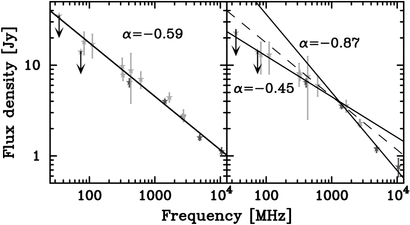
Figure 3: Integrated radio continuum spectrum of DA 495. Flux densities taken from the literature are displayed in gray and those determined in this publication in black. The left panel shows a spectrum constructed from the measured flux densities of Table 2. The indicated line, corresponding to ${\alpha}={-0.59}$, is a fit to all plotted points. The right panel shows the spectrum after allowance for the contribution of compact sources and the superimposed H II region. The solid lines corresponding to ${\alpha}={-0.45}$ and ${\alpha}={-0.87}$ are fits to points below and above 1 GHz respectively (see Section 3.2). The dashed line corresponds to ${\alpha}={-0.59}$, the fit from the left panel. The lengths of the arrows denoting the upper limits are not intended to indicate error estimates.

DA 495, while an outlier among PWNe, is without doubt a member of that class. Its radio appearance, first seen in the high-resolution images of Landecker & Caswell (1983), has the signature of a PWN, a central concentration of emission smoothly declining with increasing radius, with no evidence of a surrounding shell (although there is a depression in intensity near its center). The only indication that it might not be a PWN is its measured radio spectral index, ${\alpha}\approx{-0.5}$ (Kothes et al., 2006b), much steeper than is usual for this class of objects, and more closely resembling that of a shell-type SNR. Nevertheless, shell remnants have steep outer edges where kinetic energy is being converted to radio emission near the shock front, while in DA 495 the emissivity distribution is centrally concentrated (Landecker & Caswell, 1983, Fig. 3) indicating that the energy source is central. Nevertheless, on the basis of the central depression in intensity, Velusamy et al. (1989) argue that DA 495 might be a shell remnant with an exceptionally thick shell formed by a reverse shock interacting with an unusual amount of slowly moving ejecta.

Recent analysis of X-ray data for DA 495, obtained from the ROSAT and ASCA archives, dramatically confirms the PWN interpretation of this object by revealing a compact central object surrounded by an extended non-thermal X-ray region (Arzoumanian et al., 2004). Analysis of Chandra data (Arzoumanian et al., 2008) shows a non-thermal X-ray nebula of extent $\sim$30″ surrounding the central compact object. The compact source is presumably the pulsar (required to power the synchrotron nebula), and we shall refer to it as such (even though pulsed emission has not been detected). In this paper we present new radio images of DA 495 which include linear polarization information. Analysis of high-resolution radio images allows us to remove superimposed sources. After this the integrated spectrum of the source exhibits a spectral break characteristic of a synchrotron nebula, and the observed parameters allow an estimate of the strength of the magnetic field within the nebula. Polarization images reveal the structure of the field within this PWN.

2 Observations and Data Analysis

The DRAO observations at 408 and 1420 MHz are part of the Canadian Galactic Plane Survey (CGPS, Taylor et al., 2003). Data from single-antenna telescopes were incorporated with the Synthesis Telescope data to give complete coverage of all structures down to the resolution limit (details of the process can be found in Taylor et al., 2003). The one exception is the polarization data at 1420 MHz, for which no single-antenna data were available. However, the telescope is sensitive to all structures from the resolution limit (${\sim}1^{\prime}$) up to $45^{\prime}$. The absence of single-antenna data is not a concern for observations of DA 495, whose full extent is $\leq 30^{\prime}$. The CGPS polarization data were obtained in four bands (1407.0, 1413.0, 1427.6, and 1434.5 MHz) each of width 7.5 MHz, allowing derivation of rotation measures (RMs) between those frequencies.

The Effelsberg observations were carried out well before this investigation began, and were retrieved from archived data. Observations at 4850 and 10550 MHz were made at different times, but in each case in excellent weather. The receiver systems, installed at the secondary focus of the telescope, received both hands of circular polarization, with two feeds at 4850 MHz and four feeds at 10550 MHz. Standard data-reduction software based on the NOD2 package (Haslam et al., 1982) was employed throughout. Data reduction relied on “software beam switching” to reject atmospheric emission above the telescope (Morsi & Reich, 1986). Here every feed is equipped with its own amplifier to allow parallel recording of data. For each pair of feeds a difference map is calculated in which disturbing atmospheric effects are largely subtracted. These dual-beam maps are restored to the equivalent single-beam map with the algorithm described by Emerson et al. (1979). To reduce scanning effects, multiple maps – coverages – of the field were observed at different parallactic angles. These scanning effects arise from instrumental offsets and drifts that produce different baselevels for each individual scan, a typical result from raster scanning. Individual coverages were combined using the “plait” algorithm (Emerson & Gräve, 1988), by destriping the maps in the Fourier domain. We also used 2695 MHz data from the Effelsberg Galactic Plane Survey (Reich et al., 1990), whose angular resolution is 4$\farcm$3.

Characteristics of the new observations of DA 495, made with the DRAO Synthesis Telescope and the Effelsberg 100-m radio telescope, are presented in Table 1.

3 Results

3.1 DA 495 in total intensity

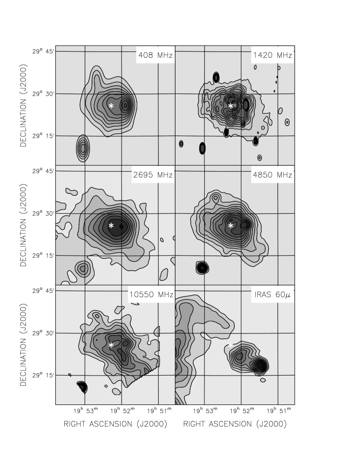
Figure 1: Total intensity maps of DA 495 at five radio frequencies, and the corresponding IRAS 60$\mu$m image. The position of the neutron star is shown in each panel by the white star. Contour levels are at: 10 K ($12\sigma$) to 100 K in steps of 10 K at 408 MHz (1 K = 8.5 mJy/beam); 0.5 K ($9\sigma$) to 5.0 K in steps of 0.5 K at 1420 MHz (1 K = 8.5 mJy/beam); 0.1 K ($5\sigma$) to 0.9 K in steps of 0.1 K at 2695 MHz (1 K = 400 mJy/beam); 5 mJy/beam ($20\sigma$) to 55 mJy/beam in steps of 5 mJy/beam at 4850 MHz (1 mJy/beam = 2.4 mK); 5 mJy/beam ($4\sigma$) to 40 mJy/beam in steps of 5 mJy/beam at 10550 MHz (1 mJy/beam = 0.5 mK); 20 MJy/sr to 28 MJy/sr in steps of 1 MJy/sr at 60$\mu$m.

Figure 1 presents total intensity images of DA 495 at 408, 1420, 4850, and 10550 MHz as well as data at 2695 MHz from the Effelsberg 11 cm survey (Reich et al., 1990) and a 60$\mu$m image from the IRAS Galaxy Atlas (IGA, Cao et al., 1997), which is part of the CGPS database. The 1420 MHz image is completely consistent with the earlier DRAO image published by Landecker & Caswell (1983), although the new image has lower noise by a factor of $\sim 3$. All the radio images show a diffuse source of full extent about $25\arcmin$. The high-resolution images at 1420, 4850, and 10550 MHz show the central depression reported by Landecker & Caswell (1983). Its position is RA(2000) = $19^{h}52^{m}10.4^{s}$, DEC(2000) = $+29\arcdeg 26\farcm 2$, and it is now apparent that the pulsar (1WGA J1952.2+2925) is not at the center of the depression (as postulated by Landecker & Caswell (1983)), but lies almost $2\arcmin$ east of it at RA(2000) = $19^{h}52^{m}17.0^{s}$, DEC(2000) = $+29\arcdeg 25\arcmin 53\arcsec$ (Arzoumanian et al., 2008). Clearly the explanation of the hole in the nebula cannot be quite as simple as a decline in emission from an aging pulsar. At larger radii, the emission drops off smoothly towards the outer edge without any sign of an outer shell at any frequency.

At 408 MHz DA 495 is quite circular in appearance. However, an extension of DA 495 to the south-west is evident at 1420 MHz and becomes increasingly prominent at higher frequencies. The IGA data shown in Figure 1 reveal an infrared source coincident with this part of the radio source. The simplest interpretation is that an H II region is superimposed on the PWN, and in the analysis we assume this to be the case.

3.2 The integrated spectrum of DA 495

We derived the integrated emission of DA 495 from each of the radio images in Figure 1, and identified a number of flux densities from the literature. All flux densities which we believe to be reliable are listed in Table 2. Flux density measurements at low radio frequencies are not easy, especially for sources of low surface-brightness; those that are available for DA 495 need to be discussed individually.

The area around DA 495 is covered by the 34.5 MHz survey of Dwarakanath & Udaya Shankar (1990), which has an angular resolution of $26\arcmin\times 44\arcmin$ at this declination. An apparently unresolved source of flux density 35 Jy is detected, offset from the position of DA 495 by 12$\farcm$5 in right ascension (to the west) and $5^{\prime}$ in declination (to the north). The offset may arise from compact sources included in the broad beam (see below). The nearby SNR G65.1+0.6 (Landecker et al., 1990) can be identified in the 34.5 MHz image. Its expected flux density at 34.5 MHz, extrapolated from higher frequency measurements, is of the order of 50 Jy, but its surface brightness is lower than that of DA 495 because of its larger size ($1.5\arcdeg\times 0.8\arcdeg$). We consider the 34.5 MHz data to be generally reliable in this area, and adopt an upper limit of 35 Jy for possible emission from DA 495 at 34.5 MHz. This is $\sim$7 times the rms sensitivity of 5 Jy quoted for the survey.

The best low-frequency data come from the new VLA Low-Frequency Sky Survey (VLSS, Cohen et al., 2007) at 74 MHz. We obtained an image of the area surrounding DA 495 from the VLSS data base. The angular resolution is $80\arcsec$, by far the best of any of our data points below 327 MHz, and fully adequate to isolate the small-diameter sources in the field. The survey is sensitive to structures up to $\sim$1^∘ in size, larger than DA 495. The survey noise is 100 mJy/beam, but in the area around DA 495 the noise is higher, about 150 mJy/beam, because of the proximity to Cygnus A. DA 495 is not visible in the 74 MHz image, not even after smoothing to a resolution of $3\arcmin$. To obtain an upper limit for the flux density at this frequency, we convolved our 1420 MHz image to this resolution, and added a scaled version to the 74 MHz image. The scaled image was just detectable when its integrated flux density was 14 Jy, and we adopted this value as the upper limit of the 74 MHz flux density of DA 495. We tested this upper limit by adding our extrapolated 1420 MHz image to areas around the position of DA 495 as well. This convinced us that we were not artificially lowering the upper limit by adding the 1420 MHz image to 74 MHz emission from DA 495 that is just slightly below the detection threshhold.

Flux densities for DA 495 at 83 and 111 MHz appear in the list published by Kovalenko et al. (1994). These observations were made with fan beams of extent a few degrees in the N–S direction. They should perhaps also be regarded as upper limits because of the possibility of confusion in the wide fan beams. We note that Kovalenko et al. (1994), while listing flux densities for DA 495, give only an upper limit for the flux density of G65.1+0.6.

Taking the measured flux densities in Table 2 at face value we derive the integrated spectrum shown in the left panel of Figure 3, fitted reasonably well over the entire frequency range by a spectral index of ${\alpha}={-0.59~{}\pm~{}0.1}$. However, the compact sources in the field around DA 495 and the superimposed H II region contaminate this spectrum. The compact sources are probably extragalactic and should mostly have spectral indices steeper than ${\alpha}={-0.59}$ (e.g. Condon, 1984); they will consequently contribute strongly to the low-frequency flux densities. The H II region will significantly contaminate the high-frequency flux densities because its spectral index is flatter than that of the non-thermal emission. We now proceed to derive an integrated spectrum for DA 495 corrected for these extraneous contributions.

We have obtained the flux densities of the three most prominent compact sources in the field shown in Figure 1 at frequencies between 74 MHz and 10550 MHz, using our new data and values from the literature. Flux densities of these sources are listed in Table 3 and their positions and fitted spectra in Table 4. The 74 MHz flux density for Source 1 is taken from the VLSS point source catalog; the flux densities for Sources 2 and 3 were derived by integration from the 74 MHz image. Flux densities for DA 495 after correction for compact sources are shown in the fourth column of Table 2.

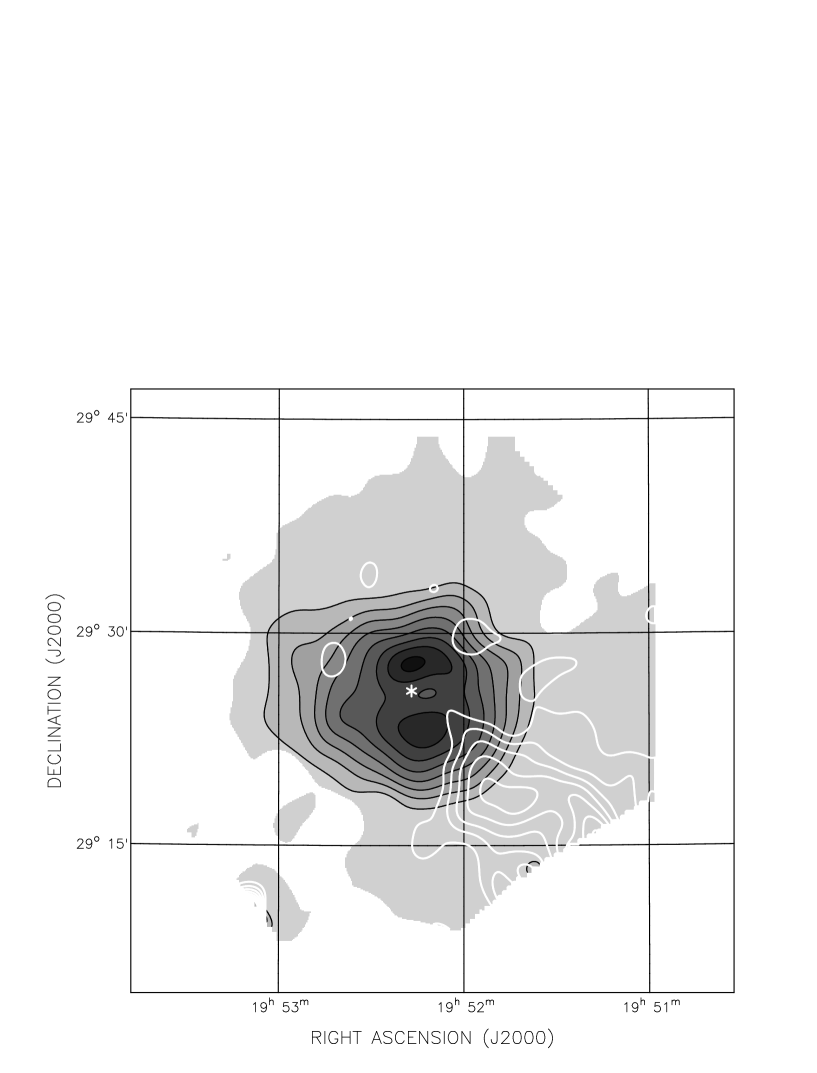
Figure 2: Separation of the total power emission at 1420 MHz into a non-thermal component (${\alpha}={-0.85}$ – shown as black contours and shading) and a thermal component (${\alpha}={-0.1}$ – white contours). Black contours are from 30 mJy/beam ($10\sigma$) to 170 mJy/beam in steps of 20 mJy/beam. White contours are from, 10 mJy/beam ($3\sigma$) to 40 mJy/beam in steps of 5 mJy/beam. The angular resolution is 2$\farcm$45 (see Section 3.2).

We expect the H II region to affect flux densities at high frequencies, because its spectral index should be ${\alpha}\approx{-0.1}$ for optically thin thermal emission. The contribution from the H II region was easily measured using our images at 1420 MHz and 10550 MHz. After convolving to an angular resolution of 2$\farcm$45, we plotted brightness temperature at 1420 MHz against that at 10550 MHz (using images from which compact sources had been subtracted) selecting only data from the north-east section of the PWN which is unlikely to be contaminated by H II region emission. The comparison implied a spectral index of $-$0.85 for this part of the PWN. Assuming that this is the spectral index of the non-thermal emission between 1420 and 10550 MHz, and that the H II region has a spectral index of $-$0.1, we made a point-by-point separation of emission into thermal and non-thermal contributions. The result is shown in Figure 2. The non-thermal emission has strong circular symmetry around the central depression, and closely resembles our 408 MHz image, where we expect the contribution of the thermal component to be negligible. The thermal component is confined to the south-west, and coincides closely with the infrared source, as expected. Because of the similarity of the non-thermal map in Fig. 2 and the 408 MHz image in Fig. 1, the coincidence of the location of the thermal source in Fig. 2 and the infrared source in Fig. 1, and the successful separation, we can be confident that our assumption of a constant spectral index for both the thermal and the non-thermal emission components is appropriate.

The contribution of the H II region to the flux density of DA 495 is $440\pm 100$ mJy at 1420 MHz. We used this value with a spectral index of $-$0.1 to calculate the contribution of emission from the H II region at frequencies of 1420 MHz and higher, and subtracted the calculated value to obtain an integrated flux density for the emission from the PWN alone. At lower frequencies we did not take the emission from the H II region into account, since the contribution of the thermal emission should become negligible and we cannot determine the frequency at which the thermal emission becomes optically thick. Flux densities for DA 495 after correction for the contribution of the H II region are shown in the fifth column of Table 2.

The right panel of Figure 3 shows the integrated spectrum of DA 495 after correction for both compact sources and the superimposed H II region. The corrected data strongly suggest a break in the spectrum of DA 495 at about 1 GHz. Fitting spectra to frequency points below 1 GHz yields a spectral index of ${\alpha}={-0.45~{}\pm~{}0.10}$. Fitting to flux densities above 1 GHz yields ${\alpha}={-0.87~{}\pm~{}0.10}$. We consider the spectrum above 1 GHz to be well determined with a two-parameter fit to 6 well defined flux density measurements. Below the break we have seven measured flux densities two of which are upper limits. There are possible errors in the spectral index below the break because of the poor angular resolution in that frequency range. The quoted error ($\pm~{}0.10$) is the formal $1\sigma$-error in the fit, but there are probably larger systematic errors which we have difficulty estimating; somewhat arbitrarily, we adopt a probable error of 0.20.

These reservations notwithstanding, we believe that this analysis has demonstrated convincingly that DA 495 has a spectral break at $1.3^{+0.3}_{-0.2}$ GHz of ${\Delta\alpha}=0.42\pm 0.22$. The spectral break may be larger than 0.4, since the low-frequency flux densities are probably upper limits, not definite measurements. Further, we have subtracted the contributions of only three compact sources. Some contribution from such sources will remain in our data, so that the plotted values are again to some extent upper limits. The location of the break frequency, however, should be well defined. Its determination is dominated by the higher frequency fluxes of the low frequency part of the spectrum. These values are well constrained, while some of the low frequency fluxes are upper limits. These affect only the slope of the spectrum below the break.

3.3 Polarization images and rotation measure

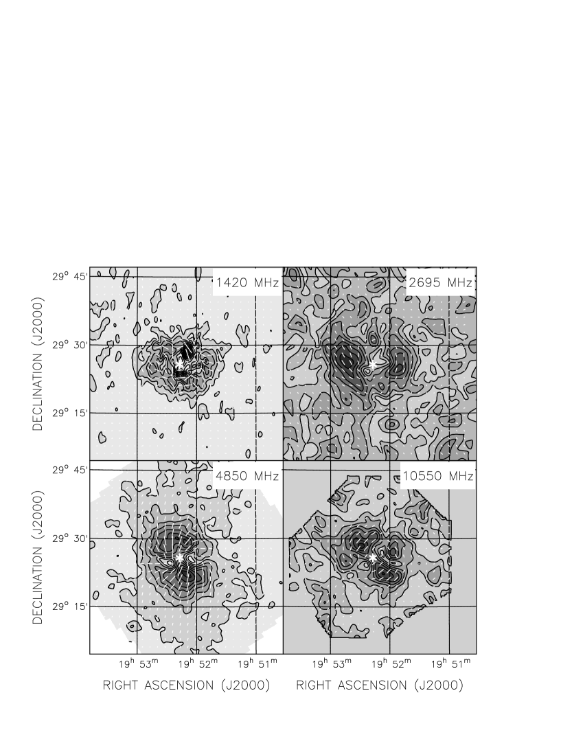
Figure 4: Polarized intensity of the emission from DA 495 and its surroundings at four frequencies, shown by contours and grayscale. The orientation of the E-field is shown by the superimposed vectors. The location of the pulsar is indicated in each panel by the star. Contour levels are at: 1.5 mJy/beam ($4\sigma$) to 12 mJy/beam at 1420 MHz; 6 mJy/beam ($2\sigma$) to 42 mJy/beam in steps of 6 mJy/beam at 2695 MHz; 1.2 mJy/beam ($6\sigma$) to 9.6 mJy/beam in steps of 1.2 mJy/beam at 4850 MHz; 0.8 mJy/beam ($2\sigma$) to 5.6 mJy/beam in steps of 0.8 mJy/beam at 10550 MHz.

Figure 4 shows our polarization images for the area around DA 495, together with data from the Effelsberg 2695 MHz survey (Duncan et al., 1999). At all frequencies the polarized emission is confined to a roughly circular region about $15\arcmin$ in diameter. No polarized emission is seen corresponding to the south-west extension, supporting the identification of this as thermal emission. No depolarization effects can be associated with this thermal emission either, and the H II region which generates it is likely more distant than DA 495.

Integrated over the entire source, the fractional polarization at the higher frequencies is about 25% (Table 5). Even at 1420 MHz the integrated polarization has dropped only to 12%, still half the value at the higher frequencies. At 1420 MHz a RM variation of only 36 rad/m² is required to rotate the polarization angle by $90\arcdeg$, and superposition of two signals whose polarization angles differ by $90\arcdeg$ produces a net signal with no apparent polarization. (At our other frequencies RM variations of about 130 rad/m² at 2695 MHz, 400 rad/m² at 4850 MHz, and 1900 rad/m² at 10550 MHz are required to generate a Faraday rotation of $90\arcdeg$.) This implies that there cannot be any rapid changes in rotation measure on scales smaller than the 1420 MHz beam, because otherwise the 1420 MHz emission would be beam depolarized.

At the two highest frequencies the polarized intensity has a remarkable bipolar distribution, seen particularly well in the 4850 MHz image (Fig. 4). Inspection shows that the bipolar structure is centered on the pulsar, immediately suggesting that the polarization structure is determined by the geometry of the magnetic field, itself tied to the pulsar. We see two prominent lobes of polarized emission, north-east and south-west of the pulsar. At the three high frequencies, from 10550 to 2695 MHz, the location of these lobes seems to rotate systematically clockwise, in the sense opposite to the rotation of polarization angle that arises from the positive RM (see below). Symmetrically on either side of the central ridge at 4850 and 10550 MHz there are small regions of low polarized intensity. The total intensity remains high at these locations, and we interpret the low fractional polarization as an indication that polarized emission generated at deeper layers within the source is superimposed on emission generated in closer layers with a significantly different polarization angle; vector averaging reduces the net polarization. This is largely an emission effect rather than a Faraday rotation effect because it is seen at high radio frequencies where Faraday rotation is low.

With linear polarization observations at four frequencies we should be able to investigate the structure of RM across the source. To this end, all observations were convolved to the lowest resolution, $4\farcm 3$, that of the 2695 MHz measurement. However, it proved impossible to calculate a RM map: at many points the calculation failed to fit a slope to the four measured polarization angles within acceptable error limits. The probable cause is “Faraday thickness” at the lower frequencies, an effect analogous to optical thickness. Depth depolarization - also known as differential Faraday rotation (Burn, 1966; Sokoloff et al., 1998) - causes the emission from the deeper levels of the source to be totally depolarized at low frequencies, so that the polarized emission we observe comes only from the nearer layers of the source. Faraday thickness seems to affect the polarization images at 2695 MHz and 1420 MHz.

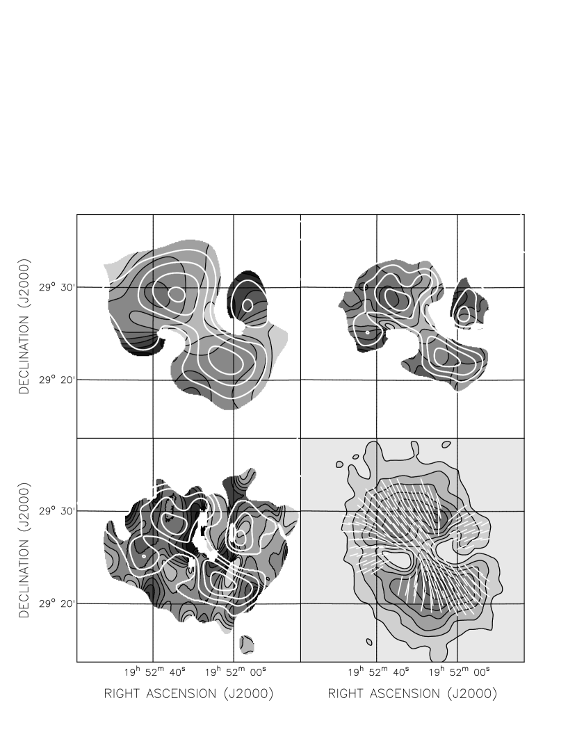
Figure 5: Upper panels: Maps of rotation measure between 4850 MHz and 10550 MHz, at the resolution of the 2695 MHz map, $4\farcm 3$ (left) and at a resolution of $2\farcm 45$ (right). Black contours represent rotation measure, with values 140, 180, 220, 260, 300, 340, 380, and 420 rad/m². White contours indicate polarized intensity at 10550 MHz at the appropriate resolution. Lower panels: Left: Map of rotation measure between the four frequency bands of the CGPS at $2\farcm 45$ (left). Contour levels are the same as in the other RM maps. Right: Map of polarized intensity at 4850 MHz shown by contours and grayscale, with levels 1.2 mJy/beam to 9.6 mJy/beam in steps of 1.2 mJy/beam. Overlaid white vectors indicate the intrinsic magnetic field directions calculated using the RM map at the top right.

Confining our attention to 4850 and 10550 MHz, we calculated a map of RM at a resolution of 4$\farcm$3, displayed in Figure 5. RM varies from 200 to 250 rad/m² on the two major emission lobes, north-east and south-west of the pulsar, to as much as 400 rad/m² in the structures to the east and west. To identify the Faraday thin and Faraday thick areas we calculated the expected polarization angles at 2695 MHz by extrapolating from the observed angles at 4850 and 10550 MHz and compared the results with values actually observed at the lower frequency. The polarization angle in the south-western lobe is as predicted, while the angle in the north-eastern lobe is about $50^{\circ}$ from the predicted value. Observed polarization angle in two patches lying approximately $4^{\prime}$ east and west of the pulsar (these patches are prominent in the 10550 MHz image of Figure 4) is about $90^{\circ}$ from the predicted value. Faraday thickness is clearly significant in this object. We also calculated a RM map between 4850 and 10550 MHz at the higher resolution of $2\farcm 45$ to examine RM fluctuations on smaller scales. The RM maps at the lower and higher resolution look virtually identical, confirming our impression that there are no strong RM fluctuations on small scales. We also calculated intrinsic polarization angles at the highest resolution and derived a map of the magnetic field (projected to the plane of the sky). This is also shown in Fig. 5.

Even though DA 495 is Faraday thick at frequencies of 2695 MHz and below, we calculated a RM map from the four bands of the CGPS 1420 MHz polarization data (Fig. 5). Surprisingly, these values of RM, which probe only the nearer layers of the source, are of the same order ($\sim 200$ rad/m²) as the values derived between 4850 and 10550 MHz where the entire line of sight through the PWN is contributing. If RM was positive right through the source the values at high frequencies should be higher than the values near 1420 MHz. This indicates that there must be regions of negative RM in the deeper layers whose effects are canceled by positive rotation nearer the front surface. A possible field configuration that could produce this is a dipole field with the dipole axis pointing away from us. Almost the entire front part of the nebula would contain magnetic field lines that point towards us, explaining why we observe only positive rotation measure at 1420 Mhz. However, deeper inside the nebula we would find magnetic field lines pointing away from us, and the Faraday rotation produced by that part of the field would partially cancel rotation produced in the near part. The exact RM configuration seen would depend on how deep we can look inside the nebula at 1420 MHz or other frequencies.

4 Discussion

4.1 Is DA 495 a PWN or a Shell SNR?

In the introduction we reviewed the arguments for the classification of DA 495 as a PWN. In brief, the emissivity is centrally concentrated and drops smoothly to zero at the outer edge without any sign of a steep shell, indicating a central energy source. This conclusion is corroborated by X-ray observations (Arzoumanian et al., 2004, 2008) that show a central compact object surrounded by a non-thermal nebula. Velusamy et al. (1989) suggest that DA 495 could be a shell remnant with an unusually thick shell. While this is a conceivable interpretation, there is no evidence of a steep outer edge to the shell and the central compact source discovered in X-ray is not located inside the radio hole, but about 2 $\arcmin$ away from it suggesting that the radio hole is not in the centre of the nebula.

This paper provides further evidence. The structure in polarized intensity is bipolar with mostly radial B-vectors at the outer edge, while for a shell-type remnant we would expect a shell structure in polarized emission with tangential B-vectors. A young shell-type SNR would have radial B-vectors, but integrated polarization would be very low and a young remnant would have bright X-ray emission coming from the expanding shell. The break in the integrated spectrum of DA 495 also provides strong evidence that the object is a PWN. Every known example of such a nebula exhibits such a break, while virtually all shell remnants have spectra characterized by a single power law. While spectral breaks have been claimed for some shell remnants, these claims are gradually melting away in the face of new data with improved sensitivity to extended emission. The only SNR where such a break has been convincingly established is S 147 (G180.0$-$1.7) which has a break in its integrated spectrum at $\sim$1.5 GHz (Fürst & Reich, 1986; Xiao et al., 2008). S 147 is a very old SNR, probably well into the isothermal stage of its evolution; it bears no resemblance to DA 495.

The only tenable conclusion is that DA 495 is a pulsar wind nebula, and we will proceed on that basis.

4.2 Distance, Size, and Emission Structure

A distance to DA 495 was measured by Kothes et al. (2004) on the basis of absorption by H I of the polarized emission from the PWN. The distance obtained, $d\approx 1.5$ kpc, was derived kinematically using a flat rotation model for the Milky Way with a Galactocentric radius of R${}_{\sun}=8.5$ kpc for the Sun and its velocity v${}_{\sun}=220$ km/s around the Galactic center. The latest measurements of the Sun’s galactocentric distance give R${}_{\sun}\approx 7.6$ kpc which is used in the new distance determination method of Foster & MacWilliams (2006, and reference therein). This method uses a model for the spatial density and velocity field traced by the distribution of H I in the disk of the Galaxy to derive a distance–velocity relation that can be used to calculate a distance to any object with a known systemic velocity. The H I absorption measurements indicate for DA 495 a systemic velocity of about $+12$ km/s. Two distances, about 1 and 5 kpc, correspond to this velocity, one closer than the tangent point and the other beyond it. Since Kothes et al. (2004) found no absorption of the PWN at the tangent point and DA 495 exhibits low foreground absorption in the X-ray observations (Arzoumanian et al., 2004, 2008) we adopt the closer distance as the more likely result. We proceed to use a distance of $1.0\pm 0.4$ kpc to determine physical characteristics of the PWN. The error contains the uncertainty in the fit and a velocity dispersion of 4 km s^-1.

To determine a reliable value for the radius we fitted a three-dimensional model of emissivity to the total-intensity observations at 1420 MHz. Our method is similar to that used by Landecker & Caswell (1983), a method developed by Hill (1967). While Landecker & Caswell (1983) centered their calculation on the depression near the middle of the nebula, we centered our new calculation on the position of the pulsar, as measured by Arzoumanian et al. (2008). In the center there is an emissivity depression with a radius of about $2\arcmin$, and so a physical radius of 0.6 pc. Outside, the emissivity is nearly constant to a radius of $7\farcm 5$, where it drops abruptly, almost to zero. This translates to an outer radius of 2.2 pc. Landecker & Caswell (1983) found that the emissivity increased from the outer edge towards the centre. This difference can be explained by the different location assumed for the centre and the contamination by the H II region (removed from our calculation but included in that of Landecker & Caswell (1983)).

Landecker & Caswell (1983) assumed that the prominent depression marked the center of the PWN, but we know now that the pulsar lies at one edge of that depression (Arzoumanian et al., 2004, 2008), not at its center. One might suppose that the pulsar has moved since it was formed, but we see from Figs. 4 and 5 that the structure in polarized intensity, and so the magnetic field structure, is centered on the pulsar. Since the radio appearance of the nebula is dominated by particles injected early in the life of the pulsar (see Section 4.3), it appears that the pulsar has not moved significantly, and we must find another explanation.

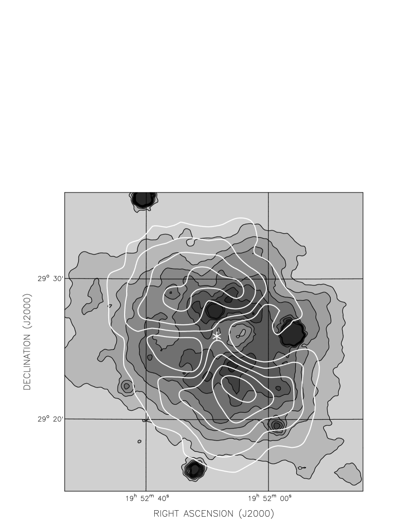
Figure 6: Map of total intensity at 1420 MHz made by merging the CGPS 1420 MHz map with a map taken from the NVSS (see Section 4.2). The resolution is about $45\arcsec$. Contour levels are at 0.8 ($8\sigma$), 1.6, 2.4, 3.2, 4.0, 4.8, and 5.6 K. Overlaid white contours indicate the polarized intensity at 4850 MHz with levels at 7, 10, 13, 16, and 19 mJy/beam.

In order to achieve higher angular resolution at 1420 MHz, we merged the 1420 MHz map from Fig. 1 with data from the NRAO VLA Sky Survey (NVSS; Condon et al., 1998). The NVSS has a resolution of about $45\arcsec$. The resulting map is shown in Fig. 6. Inspection of Fig. 6 shows evidence of a second less obvious depression in total intensity, at RA(2000) = 19^h 52^m 33^s, DEC(2000) = 29^∘ 26^′. This eastern depression is further from the pulsar than the more obvious, and deeper, hole to the west, and the nebula appears to extend to slightly larger radius beyond the eastern hole. Nevertheless, we regard the eastern depression as a significant feature. In order to produce these two emissivity depressions, there must be a region around the pulsar which is relatively free of magnetic field and/or particles. This brings to mind the Crab Nebula’s “synchrotron bays”. Fesen et al. (1992) ascribe them to an equatorial torus of material ejected by the progenitor star before it exploded. They suggest that the magnetic field of the nebula is wrapped around this torus preventing relativistic particles from entering it. A saddle-shaped depression in total power emission that connects the two holes in DA 495 (see Fig. 6) supports a torus as an explanation for these features. In the Crab Nebula the synchrotron bays are located at the edge of the emission region, but DA 495 is probably much older and the nebula has had time to flow around the torus. The distance between the two holes is about $5\arcmin$ translating to 1.45 pc at a distance of 1 kpc. This indicates an average expansion velocity of about 70 $\frac{10000\,yr}{t}$ km/s, where $t$ is the age of DA 495. For an age of 10000 yr this expansion velocity would be about 10 % of that of the Crab Nebula’s synchrotron bays, which are expanding at about 900 and 600 km/s for the western and eastern bay respectively (Fesen et al., 1992). We cannot completely rule out that movement of the pulsar is responsible for the off-center location of the pulsar between the two holes, but a difference in expansion velocity between the two sides, similar to that observed in the Crab Nebula, could explain this asymmetry.

4.3 The Nature of the Spectral Break

To investigate the nature of the break in the radio spectrum of DA 495 we first estimate the nebula’s age by comparing its energetics with the properties of other PWNe of known age. We assume for the moment that the pulsar has a symmetrical pulsar wind and that equipartition between particle and magnetic field energies has been established. We follow the analysis made by Kothes et al. (2006a) of the PWN G106.65+2.96, although, unlike that case, we have no information on the characteristic age of the DA 495 pulsar, which has not been detected. Nevertheless, we can get an estimate of the current energy loss rate of the pulsar from Arzoumanian et al. (2008): $\dot{E}_{\rm DA\,495}\approx 10^{35}$ erg/s. We now confine our attention to pulsars in historical SNRs for which we know the exact age, the Crab Nebula (SN 1054), 3C 58 (SN 1181), and G11.2$-$0.3 (SN 386) (Green, 2004). We also add three pulsar wind nebulae for which Kothes et al. (2006a) have calculated the real ages from the location of the cooling breaks in their radio spectra. We extrapolate their evolution to $\dot{E}_{\rm DA\,495}$ to determine possible properties of the pulsar in DA 495.

The evolution of the energy loss rate, $\dot{E}$, of a pulsar is defined by (e.g. Pacini & Salvati, 1973):

$$\dot{E}(t)=\frac{\dot{E_{0}}}{(1+\frac{t}{\tau_{0}})^{\beta}},$$ (1)

where $\beta$ is related to the nature of the braking torque ($\beta=\frac{n+1}{n-1}$, and $n$ is the braking index of the pulsar), $t$ is the real age of the pulsar, $\dot{E_{0}}$ is its energy loss rate at the time it was born, and $\tau_{0}$ is its intrinsic characteristic age ($\tau_{0}=\frac{P_{0}}{2\dot{P}_{0}}$, where $P_{0}$ is the period of the pulsar at the time it was born). Using the information about the current characteristic age $\tau$ and $\dot{E}$ for the six pulsars taken from the ATNF Pulsar Catalogue (Manchester et al., 2005) and their real age we can derive their initial parameters, $\tau_{0}$ and $\dot{E}_{0}$. For the Crab Pulsar and the pulsar in Vela X the braking indices are known, yielding a $\beta$ of 2.3 (Lyne et al., 1988) and 6.0 (Lyne et al., 1996), respectively. For the other four pulsars we assume a pure dipole field, implying a $\beta$ of 2. For Vela X the age depends on the assumed value of $\beta$, since we calculate it from the spectral break frequency. The resulting intrinsic pulsar properties are listed in Table 7. To indicate how much our calculations depend on this factor we used different values of $\beta$ as indicated in Table 7. Using equation 1 and taking the energy loss rate of the pulsar in DA 495 as $\dot{E}_{\rm DA\,495}\approx 10^{35}$ erg/s, we can calculate the current age, $t_{\rm DA\,495}$, of the nebula and the current characteristic age, $\tau_{\rm DA\,495}$, of its pulsar using the initial values for each of the six pulsars. The results are given in Table 8. For the Crab and the Vela X pulsars we extrapolated the energy loss rate with two different $\beta$ values as indicated in Table 8. Whatever basis we adopt for the calculation, the age of DA 495 exceeds 20,000 yr, which makes this nebula an old object. This derived age is valid regardless of the mechanism responsible for the break in the radio spectrum. All known PWNe detected at radio wavelengths contain energetic pulsars, so the low energy loss rate of the DA 495 pulsar is in all likelihood the result of age, not of intrinsically low energy.

We will now proceed by examining the different possibilites for a spectral break in the synchrotron spectrum of a pulsar wind nebula. Virtually all PWNe exhibit breaks in their spectra, at frequencies ranging from X-rays to a few GHz. Table 6 lists the break frequencies that have been identified to date. The spectral break in DA 495 occurs at 1.3 GHz, significantly lower than for any other pulsar wind nebula. A spectral break in a PWN can arise in two ways: it may reflect a break in the injected electron spectrum, and so be a mostly pulsar-dependent effect, or it may arise from synchrotron cooling, in which case the break frequency depends on the magnetic field strength and the age of the relativistic electrons in the nebula. Of course, both mechanisms should be at work in all PWNe. The suspected nature of each spectral break is indicated in Table 6.

We first consider the possibility that the break in the radio spectrum results from a break in the injected electron spectrum. Such breaks in the spectra of PWNe are known (e.g. in the Crab Nebula and 3C 58), but they are imperfectly understood. Since the electron population in the nebula is dominated by early injection, the break must have been created early in the life of the pulsar. The energy at which the break occurs depends on conditions in the area in which electrons are accelerated. Its location in the electron spectrum remains relatively fixed throughout the life of the nebula. In contrast, a break due to cooling, starts at high energy and moves with time towards lower energies (e.g. Weiler & Panagia, 1980) ultimately perhaps passing by the break produced by the injected spectrum. If the magnetic field decays with time, through expansion or other causes, both kinds of break will migrate towards lower frequencies in the radio spectrum. Their relative positions will not be affected.

A likely location for an injected break is at the energy where the electron acceleration timescale equals the synchrotron loss time, which is in essence a kind of cooling break. The difference between this situation and the normal synchrotron cooling break is that the number of high energy electrons is never high at any stage. Thus, the synchrotron spectrum should steepen by much more than the 0.5 typical of normal synchrotron cooling, which is actually the case for the intrinsic breaks identified in other PWNe. For DA 495 we found that the spectrum steepens by about 0.4.

There are two other arguments that make an injected break an unlikely interpretation for the break in the radio spectrum of DA 495. First, the X-ray synchrotron spectrum has a spectral index of $-0.63\pm 0.27$ (Arzoumanian et al., 2008, calculated from the photon index $\Gamma$: $\alpha=-(\Gamma-1)$), flatter than the synchrotron radio spectrum above the break ($-$0.87). This is impossible if the radio break arises from an injected break. The only mechanism that can affect the synchrotron spectrum beyond an intrinsic break is cooling or some other energy loss effect, which can only steepen the spectrum but cannot flatten it. A new round of particle acceleration late in the life of the PWN, an unlikely event, would affect low-energy and high-energy electrons alike. Second, there is no injected break frequency known that is even remotely as low as the 1.3 GHz we have found in DA 495.

We now consider the possibility that the break at 1.3 GHz is caused by synchrotron cooling. We will assume that the magnetic field throughout DA 495 is relatively constant or at least that there is a dominating magnetic field creating the cooling break. There are several lines of evidence supporting this assumption. First, our calculation of the synchrotron emissivity from the total-intensity images shows that emissivity is nearly constant in the majority of the nebula (Section 4.2). Second, the break in the total spectrum is very sharp and there is no significant variation of spectral index across the source (DA 495 has the same appearance at all radio frequencies, see also section 3.2: the separation into thermal and non-thermal components). Whatever the cause of the spectral break, it is the magnetic field that translates a break in the electron energy spectrum to a break in the emission spectrum. If the magnetic field varied significantly, the break would be smeared across a wide range of frequency; the break frequency has a very strong dependence on field strength (see Equation (2) below).

Chevalier (2000) found that the cooling frequency, $\nu_{c}$, corresponding to $\gamma$ (the Lorentz factor of the electron) at which the electrons are able to radiate their energy over the age of a PWN, is defined by

$$\nu_{c}[{\rm GHz}]=1.187\cdot B^{-3}[{\rm G}]\cdot t^{-2}[{\rm yr}],$$ (2)

where $B$ is the magnetic field strength inside the synchrotron nebula. Using the break frequency of $\nu_{c}\approx 1.3$ GHz and the various interpolated ages, $t_{\rm DA\,495}$, we can calculate $B_{\rm{req}}$, the required magnetic field inside the nebula (Table 8). Integrating equation (1) over the age of the nebula gives the total energy inside it and, assuming equipartition and a circular structure, we can calculate the magnetic field, $B_{\rm{max}}$. We denote this field value $B_{\rm{max}}$ because we have not accounted for any energy loss in the course of the evolution of the PWN. Comparing the results based on the six pulsars listed in Table 8, we see that it is only in the calculation based on the Crab pulsar and the pulsar in Vela X that the maximum magnetic field exceeds the magnetic field required for the spectral break. If our assumption is valid, then the pulsar in DA 495 must have been very energetic with a high energy loss rate at the time of formation, like the Crab pulsar or the pulsar in Vela X. Given the age of the Vela supernova remnant and the fact that $B_{\rm{max}}$ is significantly higher than $B_{\rm{req}}$ for any $\beta$ it is more reasonable to assume that the pulsar in DA 495 is an older version of the Vela pulsar. If we shrank the Vela X nebula with its current energy content to the size of DA 495, its cooling break at 100 GHz would decrease to about 2.5 GHz due to the resulting increase in the magnetic field strength. A few thousand years later the break frequency would reach 1.3 GHz.

Even though we cannot completely rule out the possibility that the break in the radio spectrum of DA 495 at 1.3 GHz is caused by a break in the injected electron spectrum, all the available evidence indicates that synchrotron cooling is the most likely explanation, and that DA 495 is probably an aging Vela X nebula. In this case DA 495 is about 20,000 yr old and contains a strong magnetic field of about 1.3 mG. This can easily account for the high rotation measure we have observed.

4.4 The magnetic field structure inside DA 495

The structure of the PWN in total intensity is very regular, especially once the confusing H II region is removed (see Figure 2). However, in polarized intensity the appearance is very different, and at the high frequencies DA 495 is very structured. Percentage polarization, even at the high frequencies, varies over a wide range across the source. The challenge faced in this section is to deduce something about the structure of the magnetic field inside DA 495 and to explain as many of the observed characteristics as possible. While we cannot uniquely determine the field configuration we show that one relatively simple and plausible model, a dipole field with a superimposed toroidal component, is consistent with the observations.

4.4.1 The foreground Faraday rotation

In Figure 7 we have plotted the foreground RM observed to all pulsars within $15\arcdeg$ of DA 495 as a function of distance from us in kpc. The pulsar data were taken from the ATNF Pulsar Catalog (Manchester et al., 2005). All pulsars within about 5 kpc have negative RM values, except for one for which ${\rm{RM}}={+7{\rm{~{}rad/m}}^{2}}$; we will disregard this exception because it lies at a Galactic latitude of $+14\arcdeg$. The negative RM values are consistent with the known local magnetic field orientation, away from the Sun. Pulsars more distant than 5 kpc have positive RMs, as expected from the well-known field reversal between the local and Sagittarius spiral arms (e.g. Simard-Normandin & Kronberg, 1979; Lyne & Smith, 1989). Averaged over the nearby pulsars the line-of-sight component of the magnetic field is around $-$2.5 $\mu$G. Using the models of Taylor & Cordes (1993) and Cordes & Lazio (2002) for the distribution of free electrons in the Galaxy, and the distance to DA 495 of 1.0 kpc we determine the average foreground dispersion measure to be ${\rm DM}\approx 15$ cm^-3 pc. With an average foreground magnetic field of $-$2.5 $\mu$G parallel to the line of sight this produces a foreground RM of $-$30 rad/m². The positive RM values determined from the emission of DA 495 must arise from Faraday rotation within the PWN itself or occur in a discrete foreground magneto-ionic object which does not itself produce enough emission to be detected in our observations. Since we find that almost all of the polarized emission from DA 495 is Faraday thick at 2695 MHz, most of the positive RM must originate in DA 495, because Faraday thickness can only be produced if the rotation is generated in the same volume elements as the polarized emission itself. A foreground object can merely rotate or beam depolarize the entire emission coming from behind it.

4.4.2 Magnetic field configurations inside DA 495

The magnetic field distribution seen in Figure 5 is the projection onto the plane of the sky of the three-dimensional field within DA 495, as deduced from our observations at 4850 and 10550 MHz on the assumption that the source is Faraday thin at these frequencies. The first impression is of a highly regular elongated magnetic field configuration with field lines following a central bar and spreading out radially to the north and south. This strongly resembles the inner part of a dipole field projected onto the plane of the sky. The field lines must close, presumably at large radius. However, in Figure 5 we are seeing only the component perpendicular to the line of sight. The relatively low percentage polarization even at very high frequencies of about 25 % - intrinsically it should be about 70 % - cannot be explained by depolarization caused by Faraday rotation, because at high frequencies this effect is negligible: a RM of 400 rad/m², the highest we have detected, rotates the polarization angle by a mere $20^{\circ}$ at 10550 MHz. Hence, the depolarization must be caused by the superposition of polarized emission generated at different points along the line of sight with intrinsically different polarization angles, averaging to a low net polarized fraction. In a pure dipole field the component perpendicular to the line of sight, which determines the observed polarization angle, does not change significantly along different lines of sight through the nebula. There must be an additional magnetic field present that also creates synchrotron emission but has an intrinsic magnetic field configuration perpendicular to, or at least very different from, the dipole field. A toroidal field component wrapped around the axis of the dipole would match that description. Toroidal field structures have been observed in Vela X (Dodson et al., 2003) and in the PWN in SNR G106.3$+$2.7 (Kothes et al., 2006a), although most other pulsar wind nebulae show only an elongated radial field, indicating the presence of a dipole. The patches of polarized emission to the east and west of the pulsar have a magnetic field structure perpendicular to that expected for a pure dipole field and could be a hint of a toroidal magnetic field. The two prominent “holes” in polarized intensity would then mark areas where the polarized emission generated by the dipole component and that generated by the toroidal component are equally strong but have orthogonal polarization angles so that the net emission is intense but unpolarized. Even though both magnetic field configurations may be present it is clear that the dipole field is the dominant one for emission, as seen in the magnetic field projected to the plane of the sky, and for Faraday rotation. If most of the RM was produced by the toroidal field one half of the nebula would show a negative RM and the other a positive one.

One possible magnetic field configuration that could explain the radio polarization observations of DA 495 is shown in Fig. 8. This is no more than a naive sketch, but it fits the available observations remarkably well. A similar combination of dipole and toroidal field components can explain the polarization appearance of other PWNe; the polarized emission structure, the magnetic field vectors projected to the plane of the sky, the fractional polarization, and the Faraday rotation structure all depend on the viewing angle and which one of the two components is dominant (Kothes et al., 2006a).

4.4.3 The apparent rotation of the polarization structure

One curious feature of the radio emission from DA 495 is the seemingly systematic rotation with frequency of almost the entire polarized emission structure. At the three higher frequencies we can see the two prominent lobes rotating from north-east and south-west at 10550 MHz to west and east at 2695 MHz. Near the center the two polarization holes (or, equivalently, the emission ridge) also rotate clockwise. At 2695 MHz we can no longer see this rotation near the center, probably because of the larger beam. This effect must be the product of depth depolarization in a highly ordered magnetic field structure.

A possible explanation is the following. At the intrinsic (zero wavelength) location of the polarization holes the magnetic field lines of the toroidal and dipole fields are perpendicular, and the polarization averages out. Close to the center of the PWN the dipole field lines are almost all parallel, while the toroidal field lines change with azimuthal angle within the torus. If the Faraday rotation of emission generated in the toroidal field differs from that generated in the dipole field then, at lower frequencies, this averaging no longer occurs at the “intrinsic” location but at a location where the dipole and toroidal field lines are at some angle other than 90^∘. The location of the holes then moves systematically with frequency, in the sense opposite to Faraday rotation, as observed.

If the apparent rotation of the polarized structure is a Faraday rotation effect, then it should show a $\lambda^{2}$ dependence, and we can test this. We define $\psi$ as the position angle of a line through the centers of the lobes ($\psi$ increasing from north to east). For 10550 MHz ${\psi}={45\arcdeg}$ and for 4850 MHz ${\psi}={15\arcdeg}$. Drawing a second line through the polarization holes, and assuming it is perpendicular to the line through the lobes, we find ${\psi}={38\arcdeg}$ at 10550 MHz and ${\psi}={10\arcdeg}$ at 4850 MHz. Averaging these estimates, we derive a “structural rotation” of about $-170$ rad/m² between 10550 and 4850 MHz and an intrinsic $\psi$ of $50\arcdeg$. As a test, we extrapolated to 2695 MHz, and predict ${\psi}={-70\arcdeg}$, which is very close to the $-90\arcdeg$ we observe. A second test comes from comparison with our RM map (Figure 5). Faraday rotation seems to be dominated by the dipole field, and the RM should then show a maximum or minimum at the center of the lobes because in those directions the angle between the line of sight and the field lines is smallest. A line from the RM peak in the north-eastern lobe to the pulsar has an angle of $55\arcdeg$ with north, comparable with the intrinsic $\psi$ of $50\arcdeg$ calculated above.

Since the spin axis of the pulsar is the only axis of symmetry in the rotating pulsar frame, we can assume that it is parallel to the axis of the nebula’s dipole field, which then would reflect the rotation-averaged pulsar field. We conclude that the spin axis of the pulsar, the main axis of the toroidal field, and the axis of the dipole magnetic field component all have an angle $\psi\approx{50\arcdeg}$ projected onto the plane of the sky. Further, the viewing angle, $\theta$, between the line of sight and the equatorial plane of the dipole (see Fig. 9), must be larger than $0\arcdeg$. At ${\theta}={0\arcdeg}$ the toroidal field component would be constant projected onto the plane of the sky and we would not observe the structural rotation effect.

4.4.4 Orientation of the dipole field

In this section we develop a simple model of the magnetic field configuration in DA 495. We test the model by computing RM along a few selected lines of sight through the nebula, and achieve plausible agreement with measurements. We have not attempted detailed modeling of the field.

At a distance of 1.0 kpc the diameter of DA 495 is 4.4 pc; we assume this is the maximum path length through the nebula. We deduced an internal field of about 1.3 mG from our comparisons with the Vela X nebula (Section 4.1 and Table 8) and we assume that the field is constant at this value throughout the nebula. We know the projected field distribution (Figure 5) and we know that the dipole field should be the dominating factor for the internal Faraday rotation. For these calculations we assume a dipole field as displayed in Figure 9. We confine our attention to the main axis of the dipole, because any toroidal component will be perpendicular to the line of sight and will not contribute to RM (and so we ignore the complication of the toroidal component). Magnetic field strength and synchrotron emissivity are assumed constant throughout the nebula (the evidence for these assumptions is presented in Sections 4.2 and 4.3), and the intrinsic polarization angle is set to be constant at all points along every line of sight through the nebula. We calculate the electron density $n_{e}$ within the nebula needed to generate the observed RM after correction for the foreground. We make this calculation for various viewing angles, $\theta$. In our calculations we are looking from the right hand side of Fig. 9 into the nebula. We consider we have succeeded if we can find an electron density within the nebula, assumed constant, and a viewing angle which together provide RM values reasonably consistent with the observed RM along different lines of sight. The foreground RM of approximately $-$30 rad/m² is taken as a measure of the acceptable uncertainty.

Consider first the appearance at ${\theta}={0^{\circ}}$. In the northern half the emission generated in the deeper levels first passes through a magnetic field that is directed away from us on the far side of the axis and then through a region where it is pointing towards us on the near side. Since the emission is generated uniformly along the line of sight, the bulk of the emission passes through the magnetic field that is pointing towards us and the resulting rotation measure is positive. However, in the bottom half the structure is reversed, and this should lead to a negative RM. We would expect to see a symmetrical RM map, positive to the north and negative to the south with peaks of RM of equal absolute value. Now consider the appearance at an angle ${\theta}>{0^{\circ}}$ as portrayed in Figure 9. For lines of sight above the center of the nebula, positive RM dominates, as above. For lines of sight passing below the center the emission from the far side of the nebula emerges with a strong positive RM because the path is long; there is some path through the near side that contributes negative rotation, and there is some reduction of net RM, but the path through the near side is relatively short, so that the final RM value remains strongly positive, indeed more positive than in the upper lobe. Our observations do show positive RM throughout, but with a higher RM value on the north-east lobe. Therefore to represent the observed situation, the field distribution in Figure 9 must be rotated by 180^∘ around the line of sight, so that the dipole is directed downwards and away from us.

In order to test whether this simple model can predict the observed properties of DA 495, we calculated the RM values that would be observed between 10550 and 4850 MHz for three different paths through the nebula, through the center and 1.2 pc above and below the center. At the center we observe a rotation measure of about 170 rad/m², which amounts to 200 rad/m² after correction for the foreground RM. At the RM peak on the north-eastern lobe, 1.2 pc above the center, we observe about 310 rad/m² and at the same distance on the south-western lobe we find about 250 rad/m². We calculated the electron density, n_e, required to produce these RM values for the three lines of sight through the nebula for varying viewing angles $\theta$. The results are displayed in Fig. 10. We find that the model, although approximate, can reproduce the observed RM values with reasonable values for the parameters. The small rectangles identify the region of satisfactory agreement. Within the limitations of our assumptions, the electron density in the nebula lies between 0.3 and 0.4 cm^-3 and the viewing angle $\theta$ is between 33^∘ and 40^∘.

In our model we assumed constant magnetic field throughout the nebula. Even though the total emissivity and hence the total magnetic field strength inside the nebula must be relatively constant, we know that the magnetic field strength in a dipole field decreases with distance from the centre. We use another simple model, going to the other extreme, to assess the effect of this assumption: we collapse all the rotation measure along the line of sight onto the central axis of the dipole. All the emission generated beyond the axis is rotated and then added to the emission from the near side. Due to the symmetry of the dipole, the collapsed RMs at the two positions above and below the centre used in our calculations would be the same. However, by changing the viewing angle $\theta$ we would change the pathlength through the nebula in front of and beyond the central axis. For constant emissivity we derive an angle $\theta$ of $10\arcdeg$, in contrast to the ${\sim}36\arcdeg$ derived above. Under both assumptions, and also under conditions of varying emissivity within the nebula, the dipole must be directed away from us towards the south.

Finally, in Fig. 11 we illustrate the three dimensional orientation of the dipole field inside DA 495 as determined in this section. On the left hand side we display the magnetic field projected to the plane of the sky. The magnetic field axis has an angle of about $50\arcdeg$ east of north and the magnetic field is pointing south-west. On the right hand side the dipole field orientation along the line of sight is shown, indicating that the dipole is pointing away from us towards the south-west.

4.5 Limits on a surrounding shell-type SNR

Is DA 495 a pure pulsar wind nebula, like the Crab Nebula, or does it have a surrounding SNR shell? With our new data we were able to search for such a shell. None was found, and we can place sensitive upper limits on any such emission. The noise in the area around DA 495 in our 1420 MHz image, which is the most sensitive we have for such a search, is about 40 mK rms. A $3\sigma$ signal would be about 1.0 mJy/beam, and we would need this peak flux density for a positive detection. If the inner edge of this shell is at the outer edge of the PWN and its shell thickness is 10%, typical for an adiabatically expanding SNR shell, the upper limit for the total flux density is about 90 mJy at 1420 MHz. An older remnant would have higher compression and a thinner shell, resulting in an even lower flux density limit. The 1 GHz flux density limit is about 100 mJy, using a spectral index of $\alpha=-0.5$, which is a typical value for a shell-type SNR. This translates to a maximum radio surface brightness of $\Sigma_{\rm 1~{}GHz}^{\rm max}=5.4\times 10^{-23}$ Watt m^-2 Hz^-1 sr^-1, slightly lower than the lowest radio surface-brightness known, that of the SNR G156.2$+$5.7 which has ${\Sigma_{\rm 1~{}GHz}}={6\times 10^{-23}}$ Watt m^-2 Hz^-1 sr^-1 (Reich et al., 1992).

The 60$\mu$m image of the DA 495 field (Fig. 1) shows infrared emission to the north-east of the SNR. We found H I in the CGPS data, which is likely related to this emission, because it exhibits a similar shape. This H I, however, is found at velocities near the tangent point, far removed from the systemic velocity of DA 495. We do not believe that any of this infrared emission is related to the SNR.

5 Conclusions

We have imaged the radio emission from the pulsar wind nebula DA 495 in total intensity and polarized emission across a range of frequencies from 408 to 10550 MHz. After correcting for the flux contribution of extraneous superimposed sources we have demonstrated that there is a break in the spectrum at about 1.3 GHz which we can convincingly attribute to synchrotron cooling. The spectral break at such a low frequency, the lowest known for any PWN, can only be produced if the pulsar originally was very energetic, with a high energy loss rate. We consider that DA 495 is an aging pulsar wind nebula which has a pulsar that in its earlier stages resembled the Crab pulsar or the pulsar in Vela X. The magnetic field inside the nebula is remarkably well-organized and has the topology of a dipole field centered on the pulsar; the field probably also has a toroidal component, wrapped around the dipole axis. The rotation measure is high, as would be expected in a nebula where the magnetic field has the high value of $\sim$1.3 mG, and the nebula becomes Faraday thick at a very high frequency. We have set a very low upper limit for the surface brightness for any shell of SNR emission surrounding DA 495. The absence of a shell implies that the SN explosion occurred in a low-density environment, and this also explains how the magnetic field structure has remained so regular to an age of $\sim$20,000 yr.

6 Acknowledgments

The Dominion Radio Astrophysical Observatory is a National Facility operated by the National Research Council. The Canadian Galactic Plane Survey is a Canadian project with international partners, and is supported by the Natural Sciences and Engineering Research Council (NSERC). This research is based on observations with the 100-m telescope of the MPIfR at Effelsberg. SSH acknowledges support by the Natural Sciences and Engineering Research Council and the Canada Research Chairs program. ZA was supported by NASA grant NRA-99-01-LTSA-070. The VLSS is being carried out by the (USA) National Radio Astronomy Observatory (NRAO) and the Naval Research Lab. The NRAO is operated by Associated Universities, Inc. and is a Facility of the (USA) National Science Foundation.

Table 1: Observation characteristics

Frequency [MHz]	408	1420	4850	10550
Telescope	DRAO	DRAO	Effelsberg	Effelsberg
Observation Date	January	January	February	January
				to July
	2002	2002	1996	1990
Half-power beam (′)	$2.9\times 5.95$	$0.82\times 1.75$	2.45	2.45a
	(R.A. $\times$ Dec.)	(R.A. $\times$ Dec.)
rms noise, $I$, [mJy/beam]	7	0.4	0.5	$<1.5^{b}$
rms noise, $PI$, [mJy/beam]		0.4	0.3	0.4
Calibrators, $I$, (Flux Density, Jy)	3C48 (38.9)	3C48 (15.7)	3C286 (7.5)	3C286 (4.5)
	3C147 (48.0)	3C147 (22.0)
	3C295 (54.0)	3C295 (22.1)
Calibrators $Q,U$		3C286	3C286	3C286
Linear Pol. [%]		9.25	11.3	11.7
Pol. Angle [$\arcdeg$]		33	33	33
Coveragesc			14	5

^a Original resolution 1$\farcm$15. Smoothed to 2$\farcm$45 for presentation.

^b Estimated. There is no region in the image entirely free of emission.

^c Effelsberg observations only.

Table 2: Integrated flux densities of DA 495

Frequency [MHz]	Beam	$S_{meas}$ [Jy]	$S_{cs-r}$ [Jy]	$S_{HII-r}$ [Jy]	reference
34.5	$26^{\prime}\times~{}44^{\prime}$	$<35.0$	$<$24.8		1
74	$1\farcm 33\times 1\farcm 33$		$<$14		5
83	$0.2^{\circ}\times~{}5.2^{\circ}$	$18\pm~{}5$	13.0 $\pm$ 5		2
111	$0.15^{\circ}\times~{}3.9^{\circ}$	$17\pm~{}5$	13.0 $\pm$ 5		2
318	$14^{\prime}\times~{}16^{\prime}$	$9.7\pm~{}2.2$	8.1 $\pm$ 2.2		3
327	1$\farcm$1 $\times$ 0$\farcm$6		$7.8\pm~{}1.0$		4
408	2$\farcm$8 $\times$ 5$\farcm$7		$6.5\pm~{}0.6$		5
430	8$\farcm$4 $\times$ 9$\farcm$6	$8.7\pm~{}4.9$	$7.5\pm~{}4.9$		3
610.5	$16^{\prime}\times~{}18^{\prime}$	$7.0\pm~{}1.5$	$6.0\pm~{}1.5$		6, 7
1420	0$\farcm$8 $\times$ 1$\farcm$6		$4.0\pm~{}0.2$	$3.6\pm~{}0.3$	5
1665	$22^{\prime}$	$4.4\pm~{}0.5$	$4.0\pm~{}0.5$	$3.6\pm~{}0.5$	7
2695	4$\farcm$3		$2.7\pm~{}0.2$	$2.3\pm~{}0.3$	8
2735	4$\farcm$9 $\times$ 5$\farcm$7	$2.8\pm~{}0.4$	$2.7\pm~{}0.4$	$2.3\pm~{}0.4$	7
4850	2$\farcm$45		$1.59\pm~{}0.1$	$1.2\pm~{}0.1$	5
10550	1$\farcm$15		$1.12\pm~{}0.1$	$0.76\pm~{}0.18$	5

Notes: $S_{meas}$ is the measured integrated flux density of DA 495. $S_{cs-r}$ is the measured flux density minus the total flux density of the three brightest compact sources (see text) appropriately scaled with frequency. For the new data presented in this paper, and for other high-resolution measurements, this is the integrated flux density of DA 495 without the compact sources. $S_{HII-r}$ is the integrated flux density minus an allowance for the H II region which overlaps the SNR (see text).

References: (1) Dwarakanath & Udaya Shankar (1990), (2) Kovalenko et al. (1994), (3) Dickel & DeNoyer (1975), (4) Velusamy et al. (1989), (5) present work, (6) Dickel et al. (1971), (7) Willis (1973), (8) Reich et al. (1990)

Table 3: Flux densities of compact sources [mJy]

Frequency, MHz	Source 1	Source 2	Source 3	Reference
74	1470 $\pm$ 180	1200 $\pm$ 400	900 $\pm$ 300	3 & 10
330	613 $\pm$ 50	711 $\pm$ 70	328 $\pm$ 30	1
365	557 $\pm$ 67	739 $\pm$ 52	294 $\pm$ 28	2
408	650 $\pm$ 80	504 $\pm$ 50	200 $\pm$ 40	3
1420	139 $\pm$ 5	280 $\pm$ 8	93 $\pm$ 5	4
1420	131 $\pm$ 5	244 $\pm$ 25	80 $\pm$ 6	5
1420	134 $\pm$ 8	288 $\pm$ 15	83 $\pm$ 6	3
2695		160 $\pm$ 32		6
4850	50 $\pm$ 10			7
4850		102 $\pm$ 15		8
4850		89 $\pm$ 10		9
4850	58 $\pm$ 10	108 $\pm$ 5	36 $\pm$ 4	3
10550	15 $\pm$ 4	60 $\pm$ 10	17 $\pm$ 5	3

References: (1) WENSS (Rengelink et al., 1997), (2) Texas (Douglas et al., 1996), (3) present work, (4) NVSS (Condon et al., 1998), (5) Landecker & Caswell (1983), (6) Reich et al. (1990), (7) MIT-GB (Langston et al., 1990), (8) 87GB (Gregory & Condon, 1991), (9) GB6 (Gregory et al., 1996), (10) VLSS (Cohen et al., 2007)

Table 4: Positions and spectra of compact sources

	Source 1	Source 2	Source 3
RA(2000)	19h 51m 52.1s	19h 53m 3.1s	19h 52m 40.8s
Dec(2000)	$29^{\circ}~{}26^{\prime}~{}7^{\prime\prime}$	$29^{\circ}~{}10^{\prime}~{}36^{\prime\prime}$	$29^{\circ}~{}35^{\prime}~{}47^{\prime\prime}$
A	5.05 $\pm$ 0.09	4.69 $\pm$ 0.07	4.58 $\pm$ 0.11
B	$-$0.92 $\pm$ 0.03	$-$0.72 $\pm$ 0.02	$-$0.83 $\pm$ 0.04

log(S[mJy]) = A + B log($\nu$[MHz])

Table 5: Integrated polarization properties

Frequency [MHz]	Polarized Intensity [Jy]	Fractional Polarization [%]
1420	$0.44\pm~{}0.02$	$12\pm~{}2$
2695	$0.59\pm~{}0.05$	$26\pm~{}4$
4850	$0.29\pm~{}0.03$	$24\pm~{}4$
10550	$0.18\pm~{}0.02$	$24\pm~{}6$

Fractional polarization is computed using integrated flux densities corrected for compact sources and the superimposed H II region. See Table 2

Table 6: Breaks in the spectra of pulsar wind nebulae

SNR	Break Frequency	injected/coolinga	reference
Crab Nebula	40 keV & 1000 Å	i	Woltjer et al. (1997)
Crab Nebula	14000 GHz	c	Strom & Greidanus (1992)
W44	8000 GHz	c	Petre et al. (2002)
Vela X	100 GHz	c	Weiler & Panagia (1980)
G29.7$-$0.3	55 GHz	i	Bock & Gaensler (2005)
3C 58	50 GHz	i	Salter et al. (1989); Green (1994)
G21.5$-$0.9	$\sim 30$ GHz	?	Salter et al. (1989)
G16.7+0.1	26 GHz	i	Bock & Gaensler (2005)
CTB 87	10 GHz	c	Morsi & Reich (1987)
G27.8$+$0.6	5-10 GHz	c	Reich et al. (1984)
G106.3+2.7	4.5 GHz	c	Kothes et al. (2006a)
DA 495	1.3 GHz	c	this paper

^a i denotes spectral break due to a break in the injected electron spectrum; c denotes spectral break due to synchrotron cooling

Table 7: Present day and birth properties of the six pulsars for which a reliable age can be found. For a description of individual parameters see Section 4.2.

SNR	Pulsar	$\tau$ [yr]	$\dot{E}$ [erg/s]	$\tau_{0}$ [yr]	$\dot{E}_{0}$ [erg/s]	$t$ [yr]
Crab Nebula	B0531+21	1270	$4.4\times 10^{38}$	320	$1.0\times 10^{40}$	950
3C 58	J0205+6449	5370	$2.7\times 10^{37}$	4550	$3.8\times 10^{37}$	820
G11.2$-$0.3	J1811$-$1925	23300	$6.4\times 10^{36}$	21680	$7.4\times 10^{36}$	1620
Vela X ($\beta=2.0$)	B0833-45	11300	$6.9\times 10^{36}$	110	$7.3\times 10^{40}$	11200
Vela X ($\beta=6.0$)	B0833-45	11300	$6.9\times 10^{36}$	3000	$2.0\times 10^{40}$	8300
G106.3+2.7	J2229+6114	10460	$2.2\times 10^{37}$	6560	$5.6\times 10^{37}$	3900
W 44	B1853+01	20300	$4.3\times 10^{35}$	13300	$1.0\times 10^{36}$	7000

Table 8: Properties of DA 495 extrapolated from birth properties of the six pulsars in Table 7.

Basis	$t_{\rm DA\,495}$ [yr]	$\tau_{\rm DA\,495}$ [yr]	$B_{\rm req}$ [mG]	$E_{\rm tot}$ [erg]	$B_{\rm max}$ [mG]
Crab Nebula ($\beta=2.0$)	100900	101200	0.45	$1.0\times 10^{50}$	0.98
Crab Nebula ($\beta=2.3$)	47600	47900	0.74	$7.8\times 10^{49}$	0.86
3C 58	84100	88700	0.51	$5.2\times 10^{48}$	0.22
G11.2$-$0.3	165000	186000	0.32	$4.5\times 10^{48}$	0.22
Vela X ($\beta=2.0$)	93900	94000	0.47	$2.5\times 10^{50}$	1.56
Vela X ($\beta=6.0$)	20000	23000	1.32	$3.8\times 10^{50}$	1.91
G106.3+2.7	149000	155000	0.35	$1.1\times 10^{49}$	0.32
W 44	28800	42100	1.03	$2.3\times 10^{47}$	0.05

Figure 7: Foreground rotation measure for all pulsars within $15\arcdeg$ of DA 495 as a function of distance from us in kpc. See Section 4.4.1 for source of data.

Figure 8: Sketch of a possible magnetic field configuration inside DA 495, which contains a dipole and a toroidal component. Dashed contours represent the polarized emission as observed at 4850 MHz.

Figure 9: Sketch of the dipole field configuration adopted as a model of one component of the magnetic field in DA 495. The field lines have been assumed to have a dipole configuration that is stretched vertically by a factor of 2.5. The direction of the magnetic field $\vec{\rm B}$ is indicated. The spin axis of the pulsar should be aligned with the dipole axis. The viewing angle $\theta$ is defined as shown. In Section 4.4.4 we consider this configuration viewed from the right.

Figure 10: The required electron density $n_{e}$ as a function of viewing angle $\theta$. The dashed lines in both panels correspond to the line of sight through the center of the dipole (Fig. 9), the lower line for the observed rotation measure of +170 rad/m² and the upper line for +200 rad/m², which is the observed value corrected for the foreground RM. The solid lines represent the line of sight through the dipole at a distance of 1.2 pc from the center, looking through the top of the dipole (left) and the bottom of it (right) as displayed in Fig. 9. The three lines were calculated from the top for rotation measures of +350, +300, and +250 rad/m². The small dotted rectangles delineate the range of parameter values for which the model can provide a reasonable match to observed values of RM.

Figure 11: Orientation of the dipole field inside DA 495, as determined in Sections 4.3 and 4.4. On the left the projection of the dipole field onto the plane of the sky is shown. On the right the line of sight orientation is indicated with view from the right hand side.

References

- Arzoumanian et al. (2004) Arzoumanian Z., Safi-Harb S., Landecker T.L., Kothes R., 2004, ApJ, 610, L101
- Arzoumanian et al. (2008) Arzoumanian Z., Safi-Harb S., Landecker T.L., Kothes R., Camilo, F., 2008, ApJ, accepted, ArXiv Astrophysics e-prints arXiv:0806.3766
- Blondin et al. (2001) Blondin J.M., Chevalier R.A., Frierson D.M., 2001, ApJ, 563, 806
- Bock & Gaensler (2005) Bock D. C.-J., Gaensler, B.M., 2005, ApJ, 626, 343
- Burn (1966) Burn, B.J., 1966, MNRAS, 133, 67
- Cao et al. (1997) Cao, Y., Terebey, S., Prince, T.A., Beichman, C.A., 1997, ApJS, 111, 387
- Chevalier (2000) Chevalier R.A., 2000, ApJ, 539, L45
- Cohen et al. (2007) Cohen A.S., Lane W.M., Cotton W.D., Kassim N.E., Lazio T.J.W., Perley R.A., Condon J.J., Erickson W.C., 2007, AJ, 134, 1245
- Condon et al. (1998) Condon J.J., Cotton W.D., Greisen E.W., Yin Q.F., Perley R.A., Taylor G.B., Broderick J.J., 1998, AJ, 115 1693
- Condon (1984) Condon J.J., 1984, ApJ, 287, 461
- Cordes & Lazio (2002) Cordes, J. M. & Lazio, T. J. W., 2002, ArXiv Astrophysics e-prints, astro-ph/0207156
- Dickel & DeNoyer (1975) Dickel J.R., DeNoyer L.K., 1975, AJ, 80, 437
- Dickel et al. (1971) Dickel J.R., Webber J.C., Yang K.S, Staff, 1971, AJ, 76, 294
- Dodson et al. (2003) Dodson R., Lewis D., McConnell D., Deshpande A. A., 2003, MNRAS, 343, 116
- Douglas et al. (1996) Douglas J.N., Bash F.N., Bozyan F.A., Torrence G.W., Wolfe C., 1996, AJ, 111, 1945
- Duncan et al. (1999) Duncan, A.R., Reich P., Reich W. Fürst E., 1999, A&A, 350, 447
- Dwarakanath & Udaya Shankar (1990) Dwarakanath K.S., Udaya Shankar N., 1990, J. Astrophys. Astr., 11, 323
- Emerson & Gräve (1988) Emerson D.T., Gräve R., 1988, A&A190, 353
- Emerson et al. (1979) Emerson D.T., Klein U., Haslam C.G.T. 1979, A&A, 76, 92
- Fesen et al. (1992) Fesen, R.A., Martin, C.L., Shull, J.M., 1992, ApJ, 399, 599
- Foster & MacWilliams (2006) Foster, T., MacWilliams, J. 2006, ApJ, in press (May, 2006, ApJ, 642)
- Fürst & Reich (1986) Fürst, E., Reich, W. 1986, A&A163, 185
- Green (1987) Green D.A., 1987, MNRAS, 225, L11
- Green (1994) Green, D.A., 1994, ApJS, 90, 871
- Green (2004) Green D.A., 2004, Bulletin of the Astronomical Society of India, 32, 335 (also available on the World Wide Web at http://www.mrao.cam.ac.uk/surveys/snrs)
- Gregory & Condon (1991) Gregory P.C., Condon J.J., 1991, ApJS, 75, 1011
- Gregory et al. (1996) Gregory P.C., Scott W.K., Douglas K., Condon J.J., 1996, ApJS, 103, 427
- Haslam et al. (1982) Haslam C.G.T., Stoffel H., Salter C.J., Wilson W.E., 1982, A&AS47, 1
- Hill (1967) Hill E.R., 1967, AuJPh, 29, 29
- Kothes et al. (2004) Kothes R., Landecker T.L., Wolleben M., 2004, ApJ, 607, 855
- Kothes et al. (2006a) Kothes, R., Reich, W., Uyanıker, B., 2006a, ApJ, 638, 225
- Kothes et al. (2006b) Kothes, R., Fedotov, K., Foster, T.J., Uyanıker, B., 2006b, A&A, 457, 1081
- Kovalenko et al. (1994) Kovalenko A.V., Pynzar A.V., Udal’tsov V.A., 1994, Astr. Rep., 38, 95