Abundances of Sr, Y, and Zr in Metal-Poor Stars and Implications for Chemical Evolution in the Early Galaxy

Abstract

Studies of nucleosynthesis in neutrino-driven winds from nascent neutron stars show that the elements from Sr through Ag with mass numbers $A\sim 88$–110 are produced by charged-particle reactions (CPR) during the $\alpha$-process in the winds. Accordingly, we have attributed all these elements in stars of low metallicities (${\rm[Fe/H]}\lesssim-1.5$) to low-mass and normal supernovae (SNe) from progenitors of $\sim 8$–$11\,M_{\odot}$ and $\sim 12$–$25\,M_{\odot}$, respectively, which leave behind neutron stars. Using this rule and attributing all Fe production to normal SNe, we previously developed a phenomenological two-component model, which predicts that ${\rm[Sr/Fe]}\geq-0.32$ for all metal-poor stars. The high-resolution data now available on Sr abundances in Galactic halo stars show that there is a great shortfall of Sr relative to Fe in many stars with ${\rm[Fe/H]}\lesssim-3$. This is in direct conflict with the above prediction. The same conflict also exists for two other CPR elements Y and Zr. The very low abundances of Sr, Y, and Zr observed in stars with ${\rm[Fe/H]}\lesssim-3$ thus require a stellar source that cannot be low-mass or normal SNe. We show that this observation requires a stellar source leaving behind black holes and that hypernovae (HNe) from progenitors of $\sim 25$–$50\,M_{\odot}$ are the most plausible candidates. Pair-instability SNe from very massive stars of $\sim 140$–$260\,M_{\odot}$ that leave behind no remnants are not suitable as they are extremely deficient in producing the elements of odd atomic numbers such as Na, Al, K, Sc, V, Mn, and Co relative to the neighboring elements of even atomic numbers, but this extreme odd-even effect is not observed in the elemental abundance patterns of metal-poor stars.

If we expand our previous phenomenological two-component model to include three components (low-mass and normal SNe and HNe) and use for example, the observed abundances of Ba, Sr, and Fe to separate the contributions from these components, we find that essentially all of the data are very well described by the new model. This model provides strong constraints on the evolution of [Sr/Fe] with [Ba/Fe] in terms of the allowed domain for these abundance ratios. This model also gives an equally good description of the data when any CPR element besides Sr (e.g., Y or Zr) or any heavy $r$-process element besides Ba (e.g., La) is used. As the stars deficient in Sr, Y, and Zr are dominated by contributions from HNe, they define the self-consistent yield pattern of that hypothecated source. This inferred HN yield pattern for the low-$A$ elements from Na through Zn ($A\sim 23$–70) including Fe is almost indistinguishable from what we had previously attributed to normal SNe. As HNe are plausible candidates for the first generation of stars and are also known to be ongoing in the present epoch, it is necessary to re-evaluate the extent to which normal SNe are substantial contributors to the Fe inventory of the Galaxy. We conclude that HNe are important contributors to the abundances of the low-$A$ elements over the history of the universe. We estimate that they contributed $\sim 24\%$ of the bulk solar Fe inventory while normal SNe contributed only $\sim 9\%$ (not the usually assumed $\sim 33\%$). This implies a greatly reduced role of normal SNe in the chemical evolution of the low-$A$ elements.

1 Introduction

In this paper we consider that the elements from Sr through Ag in metal-poor stars represent the products of nucleosynthesis in neutrino-driven winds from forming neutron stars. This approach allows us to obtain information on the stellar sources that contributed to the chemical enrichment of the interstellar medium (ISM) in the Galaxy and the intergalactic medium (IGM) at early and recent times. We previously proposed a phenomenological two-component model (Qian & Wasserburg 2007; hereafter QW07) to account for the abundances of heavy elements in metal-poor stars. That model focused on the elements commonly considered to be produced by the generic “$r$-process”. It specifically attributed all the elements from Sr through Ag in metal-poor stars to the charged-particle reactions (CPR) in the neutrino-driven winds from nascent neutron stars and used this as a diagnostic of the sources for these CPR elements. In contrast, the true $r$-process elements (e.g., Ba and higher atomic numbers) are produced by extensive rapid neutron capture. It was assumed in the two-component model that Fe was only produced by normal supernovae (SNe) from progenitors of $\sim 12$–$25\,M_{\odot}$, which leave behind neutron stars, and that the heavy $r$-process elements ($r$-elements) with mass numbers $A>130$ were formed in low-mass SNe from progenitors of $\sim 8$–$11\,M_{\odot}$, which also leave behind neutron stars but produce no Fe. Thus the CPR elements would be produced by both low-mass and normal SNe and the corresponding yields were estimated (QW07). It follows that if these SNe were the only sources, then the presence of Fe should always be associated with that of the CPR elements. A more extensive study of the available observational data shows that some low-metallicity stars have Fe but essentially no Sr. In particular, Fulbright et al. (2004) found a star with ${\rm[Fe/H]}=\log{\rm(Fe/H)}-\log{\rm(Fe/H)}_{\odot}=-2.88$ and $\log\epsilon({\rm Sr})=\log({\rm Sr/H})+12<-2.6$ in the dwarf galaxy Draco. From the two-component model we would have estimated $\log\epsilon({\rm Sr})=-0.28$ for this star, which is far above the observational upper limit. These results clearly indicate that if the CPR elements are always produced during the formation of neutron stars, then there must be an additional stellar source contributing Fe that does not leave behind neutron stars, or else the above model for the production of the CPR elements is in error.

Utilizing a more extensive data base than QW07 and especially treating the data on stars very deficient in Sr, Y, and Zr relative to Fe at ${\rm[Fe/H]}<-3$, the present paper will show that a third source in addition to the two sources (low-mass and normal SNe) in the model of QW07 is required to account for the elemental abundances in metal-poor stars. It will be argued that the third source producing Fe but no CPR elements is most likely associated with hypernovae (HNe) from progenitors of $\sim 25$–$50\,M_{\odot}$, which leave behind black holes instead of neutron stars. It is then shown that essentially all of the stellar data on elemental abundances at ${\rm[Fe/H]}\lesssim-1.5$ can be decomposed in terms of three distinct types of sources. This decomposition also identifies a yield pattern for the elements from Na through Zn including Fe that is attributable to HNe. An important conclusion is that this HN yield pattern is almost indistinguishable from what is attributed to normal SNe. Further, the discovery of extremely energetic HNe associated with gamma-ray bursters (e.g., Galama et al. 1998; Iwamoto et al. 1998) in the present universe requires that contributions from this source must be considered both in early epochs and on to the present. This leads to a reassessment of the contributions from different sources to the Galactic Fe inventory, which shows that ongoing HNe must play an important role and that the usual attribution of $\sim 1/3$ of the solar Fe inventory to normal SNe is not valid.

We aim to present a phenomenological three-component (low-mass and normal SNe and HNe) model for the chemical evolution of the early Galaxy that may provide a quantitative, self-consistent explanation for many of the results from stellar observations. We focus on three groups of elements: the low-$A$ elements from Na through Zn ($A\sim 23$–70), the CPR elements from Sr through Ag ($A\sim 88$–110), and the heavy $r$-elements ($A>130$, Ba and higher atomic numbers). In §2 we give a brief outline of the two-component model of QW07 with low-mass and normal SNe represented by the $H$ and $L$ sources, respectively. In §3 we present the data on abundances of Sr and Ba as well as Y and La for a large sample of metal-poor stars, and show that the two-component model fails at ${\rm[Fe/H]}\lesssim-3$ and that an additional source producing Fe but no Sr or heavier elements is required to account for the data at such low metallicities. This source is identified with HNe. It is then shown that the extended three-component model with HNe, $H$, and $L$ sources gives a good representation of nearly all the data on the CPR elements Sr, Y, and Zr, but leads to the conclusion that the HN yield pattern is indistinguishable from that of the $L$ source for all the low-$A$ elements. Considering that HNe not only represent the first massive stars (Population III stars) but also must continue into the present epoch, we reinterpret the yields attributed to the hypothetical $L$ source as the combined contributions from normal SNe, which we designate as the $L^{*}$ source, and HNe. In §4 we show that the three-component model with HNe, $H$, and $L^{*}$ sources gives a very good representation of essentially all the data on the CPR elements Sr, Y, and Zr and further discuss the characteristics of these sources and their roles in the chemical evolution of the universe. We give our conclusions in §5.

2 The Two-Component Model with the $H$ and $L$ Sources

The two-component model of QW07 was based on the observations of elemental abundances in metal-poor stars and a basic understanding of stellar evolution and nucleosynthesis. It was directed toward identifying the stellar sources for the heavy $r$-elements. The following are the key assumptions and inferences of this model:

(1) The heavy $r$-elements must be produced by an $H$ source that contributes essentially none of the low-$A$ elements including Fe. The $H$ source is most likely associated with low-mass SNe from progenitors of $\sim 8$–$11\,M_{\odot}$ that undergo O-Ne-Mg core collapse.

(2) The low-$A$ elements are produced by an $L$ source associated with normal SNe from progentiors of $\sim 12$–$25\,M_{\odot}$ that undergo Fe core collapse. (It was assumed that this source provided $\sim 1/3$ of the bulk solar Fe inventory.)

(3) The so-called light “$r$”-elements from Sr through Ag, especially Sr, Y, and Zr, in metal-poor stars must have been produced by CPRs in the $\alpha$-process (Woosley & Hoffman, 1992) that occurs as material expands away from a nascent neutron star in a neutrino-driven wind (e.g., Duncan et al. 1986). Thus, the CPR elements are not directly related to the $r$-process (i.e., they are not the true $r$-elements). Instead, their production is a natural consequence of neutron star formation in low-mass and normal SNe associated with the $H$ and $L$ sources, respectively, as proposed by QW07.

The above points were incorporated in the two-component model of QW07 to account for the elemental abundances in metal-poor stars. For ${\rm[Fe/H]}\lesssim-1.5$, Type Ia SNe (SNe Ia) associated with low-mass stars (typically of several $M_{\odot}$) in binaries had not contributed significantly to the Fe group elements in the ISM. Similarly, there were no significant contributions to Sr and heavier elements in the ISM of this early regime from the $s$-process in asymptotic giant branch (AGB) stars. Thus, it was considered in QW07 that for ${\rm[Fe/H]}\lesssim-1.5$, the $H$ source is solely responsible for the heavy $r$-elements such as Eu and the $L$ source is solely responsible for the low-$A$ elements such as Fe while both sources produce the CPR elements. The yield pattern for the prototypical $H$ source was taken from the data on a star (CS 22892–052, Sneden et al. 2003) with extremely high enrichment in the heavy $r$-elements relative to the low-$A$ elements. In contrast, the yield pattern for the prototypical $L$ source was taken from the data on a star (HD 122563, Honda et al. 2006) with very little enrichment in the heavy $r$-elements relative to the low-$A$ elements and the abundances of the latter elements in this star were attributed to the $L$ source only. For this two-component model, the (number) abundance of an element E in the ISM at ${\rm[Fe/H]}\lesssim-1.5$ can be calculated as

$$\left(\frac{\rm E}{\rm H}\right)=\left(\frac{\rm E}{\rm Eu}\right)_{H}\left(\frac{\rm Eu}{\rm H}\right)+\left(\frac{\rm E}{\rm Fe}\right)_{L}\left(\frac{\rm Fe}{\rm H}\right),$$ (1)

where (E/Eu)_H and (E/Fe)_L are the (number) yield ratios of E to Eu and Fe for the $H$ and $L$ sources, respectively. Given these yield ratios, the abundances of all the other elements (relative to hydrogen) in a star can be obtained from the above equation using only the observed abundances of Eu and Fe in that star. The results from the above model were in good agreement with the data on a large sample of metal-poor stars. We note that so long as there are no significant $s$-process contributions to the ISM (which is the case for ${\rm[Fe/H]}\lesssim-1.5$) or the star has not undergone mass transfer from an AGB companion in a binary, the element Ba can also be used as a measure of the $r$-process contributions. The yield ratios (E/Eu)_H and (E/Fe)_L for the heavy $r$-elements and the CPR elements, as well as the yield ratios (E/Ba)_H for the CPR elements, are given in Tables 1 and 2.

We emphasize the phenomenological nature of the two-component model and its extension presented below. As discussed above, the yield patterns for the $H$ and $L$ sources were taken from the observed abundance patterns in two template stars. The validity of the model should be judged by its predictions for the abundances in other metal-poor stars. Insofar as the predictions agree with the data, the model can be considered to have identified some key characteristics of nucleosynthesis in the relevant stellar sources. This approach cannot replace the ab initio models of stellar nucleosynthesis, but is complimentary to the latter.

We note that the production of the low-$A$ elements including Fe in normal SNe from progentiors of $\sim 12$–$25\,M_{\odot}$ ($L$ source) is demonstrated by extensive modeling of SN nucleosynthesis (e.g., Woosley & Weaver 1995; Thielemann et al. 1996; Chieffi & Limongi 2004), and so is the production of the CPR elements in the neutrino-driven wind associated with neutron star formation ($H$ and $L$ sources; e.g., Meyer et al. 1992; Takahashi et al. 1994; Woosley et al. 1994; Hoffman et al. 1997). However, the theoretical yields of the low-$A$ elements, especially the Fe group, are subject to the many uncertainties in modeling the evolution and explosion of massive stars. In the absence of a solid understanding of the SN mechanism, the explosion is artificially induced and the associated nucleosynthesis is parametrized by a “mass cut” (e.g., Woosley & Weaver 1995) or constrained to fit the yields of ⁵⁶Ni inferred from SN light curves (e.g., Chieffi & Limongi 2004). For the CPR elements, no reliable quantitative yields are yet available. QW07 concluded that the neutrino-driven wind does not play a significant role in the production of the heavy $r$-elements and suggested that another environment with rapid expansion timescales inside low-mass ($\sim 8$–$11\,M_{\odot}$) SNe from O-Ne-Mg core collapse ($H$ source) is responsible for making these elements. Subsequent work by Ning et al. (2007) showed that the propagation of a fast shock through the surface layers of an O-Ne-Mg core can provide the conditions leading to the production of the heavy $r$-elements. However, the required shock speed is not obtained in the current SN models (Janka et al., 2007) based on the pre-SN structure of a $1.38\ M_{\odot}$ core calculated by Nomoto (1984, 1987). Clearly, more studies of the pre-SN evolution of O-Ne-Mg cores and their collapse are needed to test whether the heavy $r$-elements can indeed be produced in the shocked surface layers of such cores. In the following we assume that low-mass SNe from O-Ne-Mg core collapse are the $H$ source solely responsible for producing the heavy $r$-elements and that the CPR elements are produced by both the $H$ and $L$ sources. At the present time, stellar models cannot calculate the absolute yields from first principles for any of the sources discussed above and some ad hoc parametric treatment is required for modeling the nucleosynthesis of these sources.

3 Failure of the Two-Component Model and Requirement of HNe

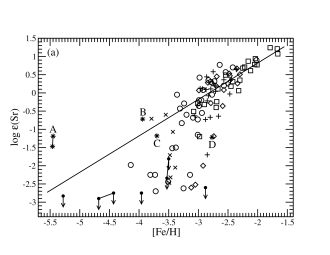
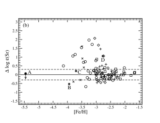
Figure 1: (a) High-resolution data on $\log\epsilon({\rm Sr})$ vs. [Fe/H] (squares: Johnson & Bolte 2002, pluses: Honda et al. 2004, diamonds: Aoki et al. 2005, circles: François et al. 2007, crosses: Cohen et al. 2008, asterisks representing stars with very high C and O abundances and anomalous abundance patterns of the low-$A$ elements: Aoki et al. 2006 (A, HE 1327–2326); Depagne et al. 2002 (B, CS 22949–037); Aoki et al. 2002 (C, CS 29498–043); Aoki et al. 2007 (D, BS 16934–002), downward arrows indicating upper limits: Christlieb et al. 2004; Fulbright et al. 2004; Frebel et al. 2007; Cohen et al. 2007; Norris et al. 2007). Symbols connected with a line indicate results for the same star assuming two different atmospheric models (subgiant vs. dwarf). Typical observational errors in $\log\epsilon({\rm Sr})$ are $\sim 0.2$–0.3 dex. The solid line is for an ISM with well-mixed $H$ and $L$ contributions. The data mostly cluster around this line but drastically depart to low $\log\epsilon({\rm Sr})$ values for ${\rm[Fe/H]}\lesssim-3$. (b) Comparison of the two-component model of QW07 and the observations in terms of $\Delta\log\epsilon({\rm Sr})\equiv\log\epsilon_{\rm cal}({\rm Sr})-\log\epsilon_{\rm obs}({\rm Sr})$ as a function of [Fe/H] for those stars shown in (a) that have observed Ba abundances. In general, the model grossly overestimates the Sr abundance below ${\rm[Fe/H]}\sim-2.7$. However, the calculated Sr abundance for HE 1327–2326 with ${\rm[Fe/H]}=-5.45$ (asterisk A) using the upper limit on its Ba abundance appears to be in good agreement with its observed Sr abundance. Measurement of the exact Ba abundance in this star will provide an extremely important test of the model.

In Figure 1a we show the data on $\log\epsilon({\rm Sr})$ from an extensive set of the available high-resolution observations over the wide range of $-5.5\lesssim{\rm[Fe/H]}\lesssim-1.5$ (squares: Johnson & Bolte 2002; pluses: Honda et al. 2004; diamonds: Aoki et al. 2005; circles: François et al. 2007; crosses: Cohen et al. 2008; asterisks: Depagne et al. 2002; Aoki et al. 2002, 2006, 2007; downward arrows indicating upper limits: Christlieb et al. 2004; Fulbright et al. 2004; Frebel et al. 2007; Cohen et al. 2007; Norris et al. 2007). All the data are for stars in the Galactic halo except for the downward arrow at ${\rm[Fe/H]}=-2.88$, which is for a star (Draco 119, Fulbright et al. 2004) in the dwarf galaxy Draco.

We now use the two-component model of QW07 to analyze the data shown in Figure 1a. We first apply equation (1) to calculate the $H$ and $L$ contributions to the solar Sr abundance assuming that the $H$ source provided all of the solar Eu abundance and the $L$ source provided 1/3 of the solar Fe abundance. Further assuming that the sun represents the sampling of a well-mixed ISM, we can show that such an ISM has [Sr/Fe]${}_{\rm mix}=-0.10$ resulting from the mixing of $H$ and $L$ contributions only (see Appendix A and Table 3). This Sr/Fe ratio corresponds to

$$\log\epsilon({\rm Sr})={\rm[Fe/H]}+2.82,$$ (2)

shown as the solid line in Figure 1a. It can be seen from this figure that the bulk of the data lie close to the solid line, but for ${\rm[Fe/H]}\lesssim-3$, almost all of the data depart greatly from this line.

There is a lack of Eu data for many stars with $[{\rm Fe/H}]<-3$. As Ba data are more readily available for such stars, we use Ba instead of Eu as the index heavy $r$-element to identify the contributions from the $H$ source (this is robust so long as there are no $s$-process contributions). Then equation (1) can be rewritten for Sr as

$$\left(\frac{\rm Sr}{\rm H}\right)=\left(\frac{\rm Sr}{\rm Ba}\right)_{H}\left(\frac{\rm Ba}{\rm H}\right)+\left(\frac{\rm Sr}{\rm Fe}\right)_{L}\left(\frac{\rm Fe}{\rm H}\right).$$ (3)

The yield ratios (E/Ba)_H and (E/Fe)_L for Sr and other CPR elements are given in Table 2. Using these yield ratios and the above equation, we calculate the $\log\epsilon_{\rm cal}{\rm(Sr)}$ values for those stars shown in Figure 1a that have observed Ba and Fe abundances. The differences $\Delta\log\epsilon({\rm Sr})\equiv\log\epsilon_{\rm cal}{\rm(Sr)}-\log\epsilon_{\rm obs}{\rm(Sr)}$ between the calculated and observed values are shown in Figure 1b. Note that for ${\rm[Fe/H]}>-2.7$, the agreement between the model predictions and the data is very good. However, for ${\rm[Fe/H]}\lesssim-2.7$, there is great discrepancy in the sense that the calculated $\log\epsilon_{\rm cal}{\rm(Sr)}$ values for many stars far exceed the observed values. It is this discrepancy that we will focus on in this paper.

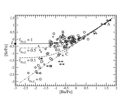
Figure 2: Evolution of [Sr/Fe] with [Ba/Fe]. Data symbols are the same as in Figure 1 except that the left-pointing arrows indicate the upper limits on [Ba/Fe]. Typical observational errors in [Sr/Fe] and [Ba/Fe] are $\sim 0.1$–0.25 dex. The curves show ${\rm[Sr/Fe]}=\log\left(10^{{\rm[Sr/Ba]}_{H}+{\rm[Ba/Fe]}}+f_{{\rm Fe},L}\times 10^{{\rm[Sr/Fe]}_{L}}\right)$ based on the three-component model with the $H$ and $L$ sources and a third source (HNe) for $f_{{\rm Fe},L}=0$ (dot-dot-dashed), 0.1 (dashed), 0.5 (dot-dashed), and 1 (solid). The parameter $f_{{\rm Fe},L}$ is the fraction of Fe contributed by the $L$ source ($f_{{\rm Fe},L}=0$ corresponds to all the Fe being from the third source). The filled circle labeled “$L$” indicates the value of [Sr/Fe]${}_{L}=-0.32$ for the $L$ source. Almost all of the data lie within the allowed region of the model. Note the presence of quite a few data on the curve for $f_{{\rm Fe},L}=0$ as well as the abundant data near the curve for $f_{{\rm Fe},L}=1$.

The large disgreement between the model predictions and the data for ${\rm[Fe/H]}\lesssim-2.7$ shown in Figure 1b is caused by assigning all the Fe to the $L$ source. If there is an additional source producing Fe but no Sr or heavier elements at such low metallicities, then equation (3) overestimates the Sr abundances. The requirement of such a source can also be seen from the Sr/Fe ratios for the stars. The yield ratio (Sr/Fe)_L corresponds to [Sr/Fe]${}_{L}=-0.32$ (see Table 3). Of the $H$ and $L$ sources, both produce Sr but only the latter can produce Fe. Thus any mixture of the contributions from these two sources should have ${\rm[Sr/Fe]}\geq-0.32$. Figure 2 shows [Sr/Fe] vs. [Ba/Fe] for those stars in Figure 1 that have observed Ba abundances or upper limits. It can be seen that many stars have ${\rm[Sr/Fe]}\ll-0.32$ and quite a few have ${\rm[Sr/Fe]}\lesssim-2$. These observations are in direct conflict with the two-component model and can only be accounted for if there is an additional source for Fe (and the associated elements) that produce none or very little of Sr and heavier elements. If we expand the framework of QW07 to include this third source, then a self-consistent interpretation of all the data may be possible.

3.1 Effects of the Third Source

In the extended model including the third source in addition to the $H$ and $L$ sources, only a fraction $f_{{\rm Fe},L}$ of the Fe is produced by the $L$ source. Then equation (3) becomes

$$\left(\frac{\rm Sr}{\rm H}\right)=\left(\frac{\rm Sr}{\rm Ba}\right)_{H}\left(\frac{\rm Ba}{\rm H}\right)+\left(\frac{\rm Sr}{\rm Fe}\right)_{L}\left(\frac{\rm Fe}{\rm H}\right)f_{{\rm Fe},L}.$$ (4)

For $f_{{\rm Fe},L}=1$ the extended model reduces to the two-component model. For $f_{{\rm Fe},L}=0$ only the $H$ source and the third source are relevant with the latter being the sole contributor of the low-$A$ elements such as Fe and the former being the sole contributor of Sr and heavier elements. Equation (4) can be rewritten as

$${\rm[Sr/Fe]}=\log\left(10^{{\rm[Sr/Ba]}_{H}+{\rm[Ba/Fe]}}+f_{{\rm Fe},L}\times 10^{{\rm[Sr/Fe]}_{L}}\right).$$ (5)

Note that the above equation represents very strong constraints on the evolution of [Sr/Fe] with [Ba/Fe] in the extended model. Whether a system starts with the initial composition of big bang debris or with an initial state inside the region defined by the curves representing equation (5) for $f_{{\rm Fe},L}=0$ and 1, it cannot have [Sr/Fe] and [Ba/Fe] values outside this region upon further evolution so long as only the $H$ and $L$ sources and the third source contribute metals.

The curves representing equation (5) for $f_{{\rm Fe},L}=0$, 0.1, 0.5, and 1 are shown along with the data on [Sr/Fe] vs. [Ba/Fe] in Figure 2. Most of the data lie between the curves for $f_{{\rm Fe},L}=0$ and 1 with a clustering of the data around the curve for $f_{{\rm Fe},L}=1$. There are also quite a few data on the curve for $f_{{\rm Fe},L}=0$. Some data lie distinctly above the curve for $f_{{\rm Fe},L}=1$. This could be partly due to observational uncertainties. We also note that all SNe associated with the $H$ and $L$ sources are assumed here to have fixed yield patterns. If there were variations in the yield ratios by a factor of several, then some “forbidden” region above the curve for $f_{{\rm Fe},L}=1$ would be accessible. In §4 we will show that with a reinterpretation of the $L$ source there is no longer a need to call upon such variabilities. In any case, we consider that the comparison between the theoretical model curves for $f_{{\rm Fe},L}=0$ to 1 and the data shown in Figure 2 justifies the extended model where a third source is producing Fe but no Sr or heavier elements.

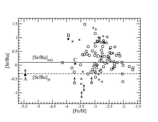
Figure 3: Data on [Sr/Ba] vs. [Fe/H]. Symbols are the same as in Figure 1 except that the upward arrows represent lower limits on [Sr/Ba]. Typical observational errors in [Sr/Ba] are $\sim 0.2$–0.3 dex. The dashed line shows the lower bound of [Sr/Ba]${}_{H}=-0.31$ for pure $H$ contributions and the solid line shows the value of [Sr/Ba]${}_{\rm mix}=0.10$ for an ISM with well-mixed $H$ and $L$ contributions. Data above the solid line represent higher proportions of $L$ contributions than in the well-mixed case. Note that considering observational uncertainties, there are no serious exceptions to the rules of Fe, Sr, and Ba production for the $H$ and $L$ sources and the third source (HNe) in the three-component model.

With no production of Sr or heavier elements assigned to the third source, the Sr/Ba ratio is determined exclusively by the $H$ and $L$ sources. As both these sources produce Sr but only the $H$ source can produce Ba, any mixture of the contributions from these two sources should have ${\rm[Sr/Ba]}\geq{\rm[Sr/Ba]}_{H}$. Figure 3 shows the data on [Sr/Ba] vs. [Fe/H] along with two reference lines, one corresponding to [Sr/Ba]${}_{H}=-0.31$ (see Table 3) and the other to [Sr/Ba]${}_{\rm mix}=0.10$ for an ISM with well-mixed $H$ and $L$ contributions (see Appendix A and Table 3). An excess of $L$ over $H$ contributions relative to the well-mixed case displaces [Sr/Ba] above the line for [Sr/Ba]_mix. It can be seen from Figure 3 that almost all of the data are compatible with the lower bound of ${\rm[Sr/Ba]}\geq{\rm[Sr/Ba]}_{H}$ and that a substantial fraction of the stars did not sample a well-mixed ISM. Excluding the lower limits, we note that some data lie below the line for [Sr/Ba]_H. However, the deviation below [Sr/Ba]_H is $\lesssim 0.4$ dex, which is comparable to the observational uncertainties and does not represent serious violation of the lower bound. It is important to note that the four stars shown as asterisks A, B, C, and D in Figures 1, 2, and 3 appear to be well behaved in terms of Sr and Ba although they have very high abundances of C and O and anomalous abundance patterns of the low-$A$ elements (see §4.3).

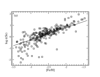
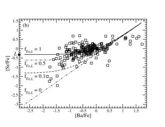
Figure 4: (a) Medium-resolution data on $\log\epsilon({\rm Sr})$ vs. [Fe/H] from the HERES survey (Barklem et al., 2005). Typical observational errors in $\log\epsilon({\rm Sr})$ are $\sim 0.3$ dex. The data in general follow the same distribution as presented in Figure 1a for the high-resolution data, where the same solid line for an ISM with well-mixed $H$ and $L$ contributions is also shown. The majority of the data cluster around the solid line but there is a great dispersion below ${\rm[Fe/H]}\sim-2.5$. (b) Evolution of [Sr/Fe] with [Ba/Fe] for the HERES sample. Typical observational errors in [Sr/Fe] and [Ba/Fe] are $\sim 0.3$ dex. The data distribution is again quite similar to the case for the high-resolution data presented in Figure 2, where the same curves are shown. A number of data lie far to the right of and below the curve for $f_{{\rm Fe},L}=0$. We consider that the corresponding stars (HE 0231–4016, HE 0305–4520, HE 0430–4404, HE 1430–1123, HE 2150–0825, HE 2156–3130, HE 2227–4044, and HE 2240–0412) may have received large $s$-process contributions. This can be tested by high-resolution observations covering more elements heavier than Ba.

To further test the robustness of the extended model including the third source, we have carried out a similar analysis of the medium-resolution data from the HERES survey of metal-poor stars (Barklem et al., 2005). This sample contains 253 stars of which eight have neither Sr nor Ba data. Five of the remaining stars were clearly recognized from their Ba/Eu ratios as having dominant $s$-process contributions (Barklem et al., 2005) and are excluded. This leaves 240 stars to be analyzed here. The data on $\log\epsilon({\rm Sr})$ vs. [Fe/H] are shown in Figure 4a analogous to Figure 1a. It can be seen that the bulk of the data again cluster around the line for an ISM with well-mixed $H$ and $L$ contributions but there are again many stars with ${\rm[Fe/H]}\lesssim-3$ showing a great deficiency in Sr. The description for the evolution of [Sr/Fe] with [Ba/Fe] by the extended model is compared with the medium-resolution data in Figure 4b. In general, these medium-resolution data are in accord with the results presented above for the high-resoltuion data shown in Figure 2, but with some exceptions. There are a number of data that lie well above the upper bound for $f_{{\rm Fe},L}=1$ (e.g., the data at ${\rm[Ba/Fe]}=-0.87$, ${\rm[Sr/Fe]}=0.68$ and ${\rm[Ba/Fe]}=-0.62$, ${\rm[Sr/Fe]}=0.70$ representing HE 0017–4838 and HE 1252–0044, respectively). This may be partly due to observational uncertainties, but it will be shown in §4 that a reinterpretation of the $L$ source raises the upper bound above essentially all the data. There are also a number of data that lie far to the right of and below the lower bound for $f_{{\rm Fe},L}=0$. We consider that the corresponding stars most plausibly have large $s$-process contributions to the Ba (these stars are: HE 0231–4016, HE 0305–4520, HE 0430–4404, HE 1430–1123, HE 2150–0825, HE 2156–3130, HE 2227–4044, and HE 2240–0412). This explanation can be tested by high-resolution observations covering more elements heavier than Ba. While not showing as clear-cut a case as the high-resolution data, the bulk of the HERES data appear to be in broad accord with the requirement of a third source producing Fe but no Sr or heavier elements as presented above.

3.2 Requirement of a Third Source from Data on Y and La as well as Zr and Ba

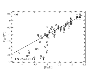
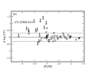
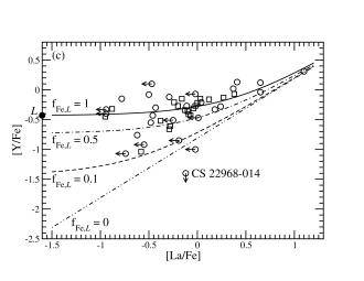
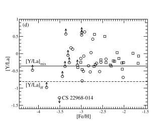
Figure 5: (a) High-resolution data on $\log\epsilon({\rm Y})$ vs. [Fe/H] (squares: Johnson 2002; circles: François et al. 2007). Downward arrows indicate upper limits. The solid line is for an ISM with well-mixed $H$ and $L$ contributions. Note that many stars with [Fe/H] $\lesssim-3$ lie below this line. (b) Comparison of the two-component model of QW07 and the observations in terms of $\Delta\log\epsilon({\rm Y})\equiv\log\epsilon_{\rm cal}({\rm Y})-\log\epsilon_{\rm obs}({\rm Y})$ as a function of [Fe/H] for the stars shown in (a). For those stars with only upper limits on the La abundance, only the $L$ contributions to Y are calculated to give the lower limits on $\Delta\log\epsilon({\rm Y})$ shown as the upward arrows. The two-component model grossly overestimates the Y abundances at ${\rm[Fe/H]}\lesssim-3$ but describes the observations very well at ${\rm[Fe/H]}>-3$. (c) Evolution of [Y/Fe] with [La/Fe] for those stars shown in (a) that have observed Y abundances. Left-pointing arrows indicate upper limits on [La/Fe]. The curves are calculated from the three-component model with the $H$ and $L$ sources and a third source (HNe) for $f_{{\rm Fe},L}=0$ (dot-dot-dashed), 0.1 (dashed), 0.5 (dot-dashed), and 1 (solid). The filled circle labeled “$L$” indicates the value of [Y/Fe]${}_{L}=-0.43$ for the $L$ source. Note that the data mostly lie between the curves for $f_{{\rm Fe},L}=0$ and 1. The anomalous star CS 22968–014 is an exception. (d) Data on [Y/La] vs. [Fe/H] for the stars shown in (c). Except for CS 22968–014, all the other stars are consistent with the lower bound of ${\rm[Y/La]}\geq{\rm[Y/La]}_{H}=-0.81$ from the three-component model. Typical observational errors in $\log\epsilon({\rm Y})$ [see (a)], [Y/Fe], [La/Fe], and [Y/La] are $\sim 0.1$–0.3 dex.

As a final test for the requirement of a third source and the robustness of the extended model including this source, we repeat the analysis using the high-resolution data on Y and La in metal-poor stars. Like Sr and Ba, these two elements represent the CPR elements and the heavy $r$-elements, respectively. The abundances of Y and La in a star are generally much lower than those of Sr and Ba, respectively. Consequently, there are much fewer data on Y and La than on Sr and Ba in metal-poor stars. On the other hand, the abundances of Y and La are less susceptible to uncertainties in the spectroscopic analysis if they can be measured and therefore, may be better indicators for the trends of chemical evolution (e.g., Simmerer et al. 2004). In Figure 5a we show the data on $\log\epsilon({\rm Y})$ from the high-resolution observations of Johnson (2002) (squares) and François et al. (2007) (circles) over the wide range of $-4.1\lesssim[{\rm Fe/H}]\lesssim-1.5$. The solid line in this figure represents

$$\log\epsilon({\rm Y})=[{\rm Fe/H}]+1.97,$$ (6)

which corresponds to [Y/Fe]${}_{\rm mix}=-0.24$ for an ISM with well-mixed contributions from the $H$ and $L$ sources only (see Appendix A and Table 3). It can be seen from Figure 5a that the bulk of the data again cluster around the solid line, but there are again many stars with [Fe/H] $\lesssim-3$ showing a great deficiency in Y.

The failure of the two-component model with the $H$ and $L$ sources as found for Sr can also be shown by comparing the Y abundances predicted from this model with the data on metal-poor stars. The yield patterns of the $H$ and $L$ sources given in Tables 1 and 2 correspond to $\log({\rm Y/La})_{H}=0.27$ and $\log({\rm Y/Fe})_{L}=-5.67$. Using these yield ratios and the La and Fe data on the stars shown in Figure 5a, we calculate the Y abundances for these stars from

$$\left(\frac{\rm Y}{\rm H}\right)=\left(\frac{\rm Y}{\rm La}\right)_{H}\left(\frac{\rm La}{\rm H}\right)+\left(\frac{\rm Y}{\rm Fe}\right)_{L}\left(\frac{\rm Fe}{\rm H}\right)$$ (7)

and show the differences $\Delta\log\epsilon({\rm Y})\equiv\log\epsilon_{\rm cal}({\rm Y})-\log\epsilon_{\rm obs}({\rm Y})$ between the calculated and observed values in Figure 5b. As many stars lack La data, their $\log\epsilon_{\rm cal}({\rm Y})$ values are calculated from the $L$ contributions only. The resulting $\Delta\log\epsilon({\rm Y})$ values represent lower limits and are shown as symbols with upward arrows [the value of $\log({\rm Y/Fe})_{L}=-5.67$ should represent the minimum value of $\log({\rm Y/Fe})=\log\epsilon({\rm Y})-\log\epsilon({\rm Fe})$ predicted for metal-poor stars based on the two-component model]. It can be seen from Figure 5b that there is again good agreement between the two-component model and the data for ${\rm[Fe/H]}>-3$ but the model tends to greatly overpredict Y abundances (by up to $\sim 1.3$ dex) for ${\rm[Fe/H]}\lesssim-3$.

As discussed using just the Sr and Ba data, the two-component model must be modified by including a third source producing Fe but no CPR or heavier elements in order to account for the observations. The effects of such a source are shown in Figure 5c for the CPR element Y and the heavy $r$-element La analogous to Figures 2 and 4b for Sr and Ba. The data on the evolution of [Y/Fe] with [La/Fe] shown in Figure 5c are for the stars shown in Figure 5a except for those with only upper limits on both Y and La abundances. The distribution of the data on Y and La with respect to the curves calculated from the three-component model for $f_{{\rm Fe},L}=0$, 0.1, 0.5, and 1 is similar to those discussed in §3.1 for the evolution of [Sr/Fe] with [Ba/Fe] and shown in Figures 2 and 4b. There is one exceptional star, CS 22968–014, which is indicated by the downward arrow labeled as such in Figure 5c. This star has an anomalously high abundance of La corresponding to $\log({\rm La/Ba})=0.7$ (François et al., 2007), which greatly exceeds the yield ratio of $\log({\rm La/Ba})_{H}=-0.71$ assumed for the $H$ source (see Table 1). If the measured La/Ba ratio were correct, then CS 22968–014 must have sampled an extremely anomalous event producing the heavy $r$-elements. However, the Ba and La abundances for this star were derived from a single line for either element (François et al., 2007), and therefore, could be in error. More observations of these two elements in this star are needed to resolve this issue. In any case, we consider that the overall comparison between the theoretical model curves for $f_{{\rm Fe},L}=0$ to 1 and the data shown in Figure 5c justifies the three-component model where the third source is producing Fe but no CPR or heavier elements.

With no production of CPR or heavier elements assigned to the third source, the Y/La ratio is determined exclusively by the $H$ and $L$ sources. Any mixture of the contributions from these two sources should have ${\rm[Y/La]}$ exceeding ${\rm[Y/La]}_{H}=-0.81$ (see Table 3). An ISM with well-mixed $H$ and $L$ contributions should have [Y/La]${}_{\rm mix}=-0.36$ (see Appendix A and Table 3). The data on [Y/La] for the stars shown in Figure 5c are displayed in Figure 5d analogous to Figure 3. It can be seen from Figure 5d that except for the anomalous star CS 22968–014 noted above, all other data are compatible with the lower bound of ${\rm[Y/La]}\geq{\rm[Y/La]}_{H}$ and that a large fraction of the stars did not sample a well-mixed ISM.

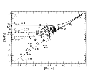
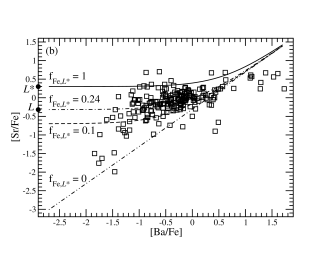
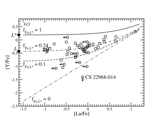
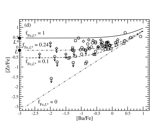
Figure 7: (a) Evolution of [Sr/Fe] with [Ba/Fe] in the three-component model with HNe, $H$, and $L^{*}$ sources compared with the high-resolution data (analogous to Figure 2). (b) The same relationships compared with the medium-resolution data (analogous to Figure 4b). (c) Evolution of [Y/Fe] with [La/Fe] compared with the high-resolution data (analogous to Figure 5c). (d) Evolution of [Zr/Fe] with [Ba/Fe] compared with the high-resolution data (squares: Johnson 2002; diamonds: Aoki et al. 2005; circles: François et al. 2007). Typical observational errors in [Zr/Fe] and [Ba/Fe] are $\sim 0.1$–0.25 dex. The parameter $f_{{\rm Fe},L^{*}}$ is the fraction of Fe contributed by the $L^{*}$ source. The filled circles labeled “$L$” indicate the (number) yield ratios of [Sr/Fe]${}_{L}=-0.32$ (a) and (b), [Y/Fe]${}_{L}=-0.43$ (c), and [Zr/Fe]${}_{L}=-0.16$ (d) for the $L$ source, while those labeled “$L^{*}$” indicate the yield ratios of [Sr/Fe]${}_{L^{*}}=0.30$ (a) and (b), [Y/Fe]${}_{L^{*}}=0.19$ (c), and [Zr/Fe]${}_{L^{*}}=0.46$ (d) for the $L^{*}$ source (see Table 3). The increase from the $L$ to the $L^{*}$ yield ratio is the same for all the CPR elements. Note that except for the data points far to the right of and below the curve for $f_{{\rm Fe},L^{*}}=0$ in (b), which may represent stars with large $s$-process contributions, and the anomalous star CS 22968–014 noted in the text, essentially all the data lie inside the allowed region bounded by the curves for $f_{{\rm Fe},L^{*}}=0$ and 1.

Based on the analysis of the Sr and Ba data as well as the Y and La data, we consider that a three-component model including a third source producing Fe but no CPR or heavier elements is adequately justified. Our analysis of the Zr and Ba data (not presented in detail here) is in full accord with the three-component model and leads to the same quantitative conclusion (see §4 and Figure 7d). We will now pursue the consequences of this approach.

3.3 HNe as the Third Source

Star formation in the early universe responsible for the enrichment of metal-poor stars is still not well understood. Simulations indicate that the first stars were likely to be massive, ranging from $\sim 10$ to $\sim 1000\,M_{\odot}$ [see Abel et al. (2002); Bromm & Larson (2004) for reviews of earlier works and Yoshida et al. (2006); O’Shea & Norman (2007); Gao et al. (2007) for more recent studies]. It is generally thought that stars form in the typical mass range of $\sim 1$–$50\,M_{\odot}$ subsequent to the epoch of the first stars. Below we assume this simple scenario of star formation and focus on considerations of nucleosynthesis to identify the stellar types for the third source.

The assumed third source produces the low-$A$ elements including Fe but no CPR elements such as Sr or heavier elements. As the CPR elements are here considered to be produced in the neutrino-driven wind from nascent neutron stars, there are two main candidates for the third source : (1) pair-instability SNe (PI-SNe) from very massive ($\sim 140$–$260\,M_{\odot}$) stars (VMSs), in which the star is completely disrupted by the explosion and no neutron star is produced, and (2) massive SNe with progenitors of $\sim 25$–$50\,M_{\odot}$, in which a black hole forms either directly by the core collapse or through severe fallback onto the neutron star initially produced by the core collapse. There is observational evidence that massive SNe have two branches: HNe and faint SNe with the latter thought to be much rarer. Compared with normal SNe, HNe have up to $\sim 50$ times higher explosion energies and $\sim 7$ times higher Fe yields while faint SNe have several times lower explosion energies and $\gtrsim 10$ times lower Fe yields [see Iwamoto et al. (1998) for interpretation of SN 1998bw as an HN, Turatto et al. (1998) for the case of SN 1997D as a faint SN, and Nomoto et al. (2006) and references therein for other studies of HNe and faint SNe]. It is important to note that HNe are ongoing events in the present universe as evidenced by the occurrences of the associated gamma-ray bursts [see e.g., Galama et al. (1998) for the discovery of SN 1998bw, an HN associated with a gamma-ray burst].

In our assumed scenario of star formation, PI-SNe can only occur at zero metallicity but HNe and faint SNe can occur at all epochs. In addition, these three types of events have very different yield patterns of the low-$A$ elements. Compared with HNe and faint SNe, PI-SNe have extremely low production of those low-$A$ elements with odd atomic numbers such as Na, Al, K, Sc, V, Mn, and Co relative to their neighboring elements with even atomic numbers (see Figure 3 in Heger & Woosley 2002). This is because unlike HNe and faint SNe that occur after all stages of core burning, PI-SNe occur immediately following core C-burning and there is not sufficient time for weak interaction to provide the required neutron excess for significant production of the low-$A$ elements with odd atomic numbers (e.g., Heger & Woosley 2002). Further, the production of the low-$A$ elements from Na through Mg relative to those from Si through Zn differs greatly between HNe and faint SNe. This is because the former elements are produced by hydrostatic burning during the pre-explosion evolution and the latter ones by explosive burning. The extremely weak explosion of faint SNe would lead to very high yield ratios of the hydrostatic burning products relative to the explosive burning products.

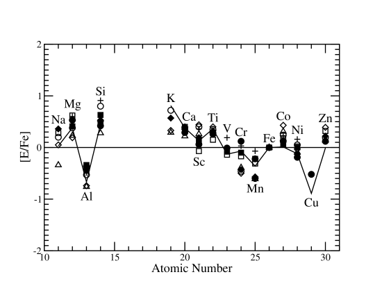
Figure 6: Comparison of the abundance patterns of the low-$A$ elements for the third source (HNe) and the $L$ source. The patterns for the third source are taken from five stars that lie on the curve for $f_{{\rm Fe},L}=0$ in Figure 2 (open square: BD $-18^{\circ}5550$, ${\rm[Fe/H]}=-2.98$, Johnson 2002; open circle: CS 30325–094, ${\rm[Fe/H]}=-3.25$, open diamond: CS 22885–096, ${\rm[Fe/H]}=-3.73$, open triangle: CS 29502–042, ${\rm[Fe/H]}=-3.14$, Cayrel et al. 2004; plus: BS 16085–050, ${\rm[Fe/H]}=-2.85$, Honda et al. 2004). Those for the $L$ source are from three stars that lie on the curve for $f_{{\rm Fe},L}=1$ in Figure 2 (filled square: BD $+4^{\circ}2621$, Johnson 2002; filled circle: HD 122563, Honda et al. 2004, 2006; filled diamond: CS 29491–053, Cayrel et al. 2004). The solid curve represents a star (BD $+17^{\circ}3248$, Cowan et al. 2002) with a relatively high value of ${\rm[Fe/H]}=-2$. Typical observational errors in [E/Fe] are $\sim 0.1$–0.25 dex. All the patterns shown are essentially indistinguishable.

The decomposition of elemental abundances in terms of three components discussed in §3.1 and §3.2 identifies those stars in which the Fe is exclusively the product of the third source. Such stars lie on the curve for $f_{{\rm Fe},L}=0$ representing the mixture of contributions from the $H$ source and the third source in Figure 2. As the $H$ source produces none of the low-$A$ elements, these elements in the stars lying on the $f_{{\rm Fe},L}=0$ curve should be attributed to the third source. The abundance patterns of these elements in five such stars (open square: BD $-18^{\circ}5550$, ${\rm[Fe/H]}=-2.98$, Johnson 2002; open circle: CS 30325–094, ${\rm[Fe/H]}=-3.25$, open diamond: CS 22885–096, ${\rm[Fe/H]}=-3.73$, open triangle: CS 29502–042, ${\rm[Fe/H]}=-3.14$, Cayrel et al. 2004; plus: BS 16085–050, ${\rm[Fe/H]}=-2.85$, Honda et al. 2004) are shown in Figure 6. It can be seen that all the abundance patterns of the low-$A$ elements assigned to the third source are quasi-uniform. By quasi-uniformity, we mean that for element E, the [E/Fe] values for different stars are within $\sim 0.3$ dex of some mean value. It is also clear that there are no drastic variations in the [E/Fe] values either between the elements with odd and even atomic numbers or between the hydrostatic and explosive burning products. We conclude that neither PI-SNe nor faint SNe can be the third source. This leaves HNe as the third source.

The abundance patterns of the low-$A$ elements in those stars that lie on the curve for $f_{{\rm Fe},L}=1$ in Figure 2 should represent the yield pattern of these elements for the hypothecated $L$ source. The patterns for three such stars (filled square: BD $+4^{\circ}2621$, Johnson 2002; filled circle: HD 122563, Honda et al. 2004, 2006; filled diamond: CS 29491–053, Cayrel et al. 2004) are compared with those assigned to the third source in Figure 6. It can be seen that the third source (now taken to be HNe) and the $L$ source are indistinguishable in terms of their assigned contributions to the low-$A$ elements. This is also reflected by the fact that essentially all the stars in the region bounded by the curves for $f_{{\rm Fe},L}=0$ and 1 shown in Figure 2 have the same quasi-uniform abundance patterns of the low-$A$ elements as established by the observations of Cayrel et al. (2004) (see §4.3 for discussion of the exceptional stars). As an example, we show in Figure 6 the pattern for BD $+17^{\circ}3248$ (solid curve, Cowan et al. 2002) with a relatively high value of ${\rm[Fe/H]}=-2$. We are thus left with a most peculiar conundrum: the yield pattern of the low-$A$ elements attributed to the third source is the same as that attributed to the $L$ source. This is the same result that we (Qian & Wasserburg, 2002) found earlier in attempting to estimate the yield patterns of the stellar sources contributing in the regime of ${\rm[Fe/H]}\lesssim-3$ using the data of McWilliam et al. (1995) and Norris et al. (2001). The recent more extensive and precise data of Cayrel et al. (2004) lead to the same conclusion.

We have associated the third source with HNe and the $L$ source with normal SNe. As HNe and normal SNe are concurrent in our assumed scenario of star formation and cannot be distinguished based on their production of the low-$A$ elements, the contributions to these elements, especially Fe, that we previously assigned to the $L$ source only may well be a combination of the contributions from both HNe and normal SNe. In this case, the Sr/Fe ratio assigned to the $L$ source represents a mixture of Sr contributions from normal SNe and Fe contributions from both HNe and normal SNe. In what follows, we designate normal SNe as the $L^{*}$ source and consider the $L$ source as a combination of HNe and the $L^{*}$ source ($L\to{\rm HNe}+L^{*}$). The apparent near identity in the abundance patterns of the low-$A$ elements attributed to HNe and the $L$ source may mean that the dominant contributor to these elements is HNe. The stellar types and the nucleosynthetic characteristics assigned to HNe, $H$, and $L^{*}$ sources are summarized in Table 4.

In our earlier efforts to decompose the stellar sources of elemental abundances at low metallicities, we recognized that there must be a source producing Fe and other low-$A$ elements but none of the $r$-elements (Qian & Wasserburg, 2002). We therefore proposed a source that only occurred in very early epochs and did not occur later. This inference, in conjunction with the rather sharp break in the observed abundances of the heavy $r$-elements at ${\rm[Fe/H]}\sim-3$, led us to propose that PI-SNe from VMSs might be the source. It was argued that VMSs were the first stars and that the very disruptive PI-SNe associated with them provided a baseline of metals to the IGM at a level of ${\rm[Fe/H]}\sim-3$. This apparent baseline was also found in damped Lyman $\alpha$ systems (Qian et al., 2002). However, in the framework of hierarchical structure formation, for halos that are not disrupted by explosions of massive stars (see §4.2), the initial rate of growth in metallicity is so rapid that it would be very rare to find stars with ${\rm[Fe/H]}<-3$ (Qian & Wasserburg, 2004). It is thus plausible that the rarity of ultra-metal-poor stars with ${\rm[Fe/H]}<-3$ results from the initial phase of rapid metal enrichment in all bound halos and is not due to a general “prompt inventory” in the IGM. In addition, as discussed above, none of the metal-poor stars with ${\rm[Fe/H]}\lesssim-3$ exhibit the abundance patterns calculated for PI-SNe, which are extremely deficient in the elements with odd atomic numbers such as Na, Al, K, Sc, V, Mn, and Co (e.g., Heger & Woosley 2002). Further, the search for ultra-metal-poor stars has shown that while stars with ${\rm[Fe/H]}<-3$ are rare, they do occur and show some evidence of elements heavier than the Fe group in their spectra (see Christlieb et al. 2002; Frebel et al. 2007 for the discovery of the two most metal-poor stars with ${\rm[Fe/H]}<-5$). Thus, low-mass stars must be able to form from a medium with ${\rm[Fe/H]}\ll-3$. Based on all the above considerations, we now must withdraw the “prompt inventory” hypothesis and must consider an IGM with widely variable “metal” content and that ${\rm[Fe/H]}\sim-3$ represents a transition to the regime where halos are no longer disrupted by the explosions of massive stars.

4 The Three-Component Model with HNe, $H$, and $L^{*}$ Sources

With the revised interpretation of the $L$ source as a combination of HNe and the $L^{*}$ source, we can relate ${\rm[Sr/Fe]}_{L}=-0.32$ (see Table 3) to the yield ratio of Sr to Fe for the $L^{*}$ source. For example, if we assume that 24% of the Fe in the $L$ mixture is from the $L^{*}$ source (see §4.1), this corresponds to ${\rm[Sr/Fe]}_{L^{*}}={\rm[Sr/Fe]}_{L}-\log 0.24=0.30$. Equation (5) now becomes

$${\rm[Sr/Fe]}=\log\left(10^{{\rm[Sr/Ba]}_{H}+{\rm[Ba/Fe]}}+f_{{\rm Fe},L^{*}}\times 10^{{\rm[Sr/Fe]}_{L^{*}}}\right),$$ (8)

where $f_{{\rm Fe},L^{*}}$ is the fraction of the Fe in a star contributed by the $L^{*}$ source. The curves representing the above equation for ${\rm[Sr/Fe]}_{L^{*}}=0.30$ and $f_{{\rm Fe},L^{*}}=0$, 0.1, 0.24, and 1 are shown along with the data in Figures 7a (high-resolution data) and 7b (medium-resolution data) analogous to Figures 2 and 4b. It can be seen from Figures 7a and 7b that essentially all the data lie inside the allowed region for the evolution of [Sr/Fe] with [Ba/Fe] bounded by the curves for $f_{{\rm Fe},L^{*}}=0$ and 1 (as mentioned near the end of §3.1, the exceptional data points far to the right of and below the curve for $f_{{\rm Fe},L^{*}}=0$ in Figure 7b most likely represent stars that received large $s$-process contributions to Ba).

Assuming that 24% of the Fe in the $L$ mixture is from the $L^{*}$ source as for Figures 7a and 7b, we obtain ${\rm[Y/Fe]}_{L^{*}}={\rm[Y/Fe]}_{L}-\log 0.24=0.19$ (see Table 3). Using this yield ratio, we show the curves representing

$${\rm[Y/Fe]}=\log\left(10^{{\rm[Y/La]}_{H}+{\rm[La/Fe]}}+f_{{\rm Fe},L^{*}}\times 10^{{\rm[Y/Fe]}_{L^{*}}}\right)$$ (9)

for $f_{{\rm Fe},L^{*}}=0$, 0.1, 0.24, and 1 along with the data in Figure 7c analogous to Figure 5d. It can be seen from Figure 7c that with the exception of the anomalous star CS 22968–014 as noted in §3.2, all other data again lie inside the allowed region for the evolution of [Y/Fe] with [La/Fe] bounded by the curves for $f_{{\rm Fe},L^{*}}=0$ and 1.

For completeness, we also show the high-resolution data on the evolution of [Zr/Fe] with [Ba/Fe] (squares: Johnson 2002; diamonds: Aoki et al. 2005; circles: François et al. 2007) in Figure 7d along with the curves representing

$${\rm[Zr/Fe]}=\log\left(10^{{\rm[Zr/Ba]}_{H}+{\rm[Ba/Fe]}}+f_{{\rm Fe},L^{*}}\times 10^{{\rm[Zr/Fe]}_{L^{*}}}\right)$$ (10)

for $f_{{\rm Fe},L^{*}}=0$, 0.1, 0.24, and 1. In the above equation, we take [Zr/Ba]${}_{H}=-0.20$ and [Zr/Fe]${}_{L^{*}}=0.46$ (see Table 3). The latter yield ratio again assumes that 24% of the Fe in the $L$ mixture is from the $L^{*}$ source as for Figures 7a, 7b, and 7c. It can be seen from Figure 7d that essentially all the data again lie inside the allowed region for the evolution of [Zr/Fe] with [Ba/Fe] bounded by the curves for $f_{{\rm Fe},L^{*}}=0$ and 1.

Based on the comparison of the theoretical model curves and the data on Sr, Y, and Zr shown in Figure 7, we consider that the three-component model with HNe, $H$, and $L^{*}$ sources provides a very good description of the elemental abundances in metal-poor stars. For an overwhelming portion of the metal-poor stars shown in this figure, their inventory of Fe and other low-$A$ elements received significant but not dominant contributions from the $L^{*}$ source (normal SNe) as indicated by the corresponding low values of $f_{{\rm Fe},L^{*}}$. We conclude that the bulk of the low-$A$ elements including Fe in metal-poor stars with ${\rm[Fe/H]}\lesssim-1.5$ was provided by HNe. This may explain why wide fluctuations in the abundance patterns of the low-$A$ elements expected from the contributions of just a few normal SNe are not actually observed. The matter remains as to what the detailed yield patterns of the $L^{*}$ source are for the low-$A$ elements. This is not easily addressable from the observations of metal-poor stars as the $L^{*}$ contributions only constitute a small fraction of the total abundances of these elements. It appears that we must rely on stellar model calculations (e.g., Woosley & Weaver 1995; Chieffi & Limongi 2004) to estimate the $L^{*}$ yield patterns of the low-$A$ elements.

A straightforward application of the three-component model is to calculate the contributions from the $H$ and $L^{*}$ sources to the solar inventory of the CPR elements. Assuming that all of the Eu in the sun was provided by the $H$ source and a fraction $f_{{\rm Fe},L^{*}}^{\odot}=0.08$ of the solar Fe inventory was provided by the $L^{*}$ source ($f_{{\rm Fe},L^{*}}^{\odot}=0.24f_{{\rm Fe},L}^{\odot}$ with $f_{{\rm Fe},L}^{\odot}=1/3$ being the fraction contributed by sources other than SNe Ia as usually assumed), we calculate the $H$ and $L^{*}$ contributions to a CPR element E in the sun from

$$\left(\frac{\rm E}{\rm H}\right)_{\odot,HL^{*}}=\left(\frac{\rm E}{\rm Eu}\right)_{H}\left(\frac{\rm Eu}{\rm H}\right)_{\odot}+\left(\frac{\rm E}{\rm Fe}\right)_{L^{*}}\left(\frac{\rm Fe}{\rm H}\right)_{\odot}f_{{\rm Fe},L^{*}}^{\odot}\ ,$$ (11)

where the yield ratios (E/Eu)_H and (E/Fe)${}_{L^{*}}$ are given in Table 2. We present the results in terms of $\log\epsilon_{\odot,HL^{*}}({\rm E})$ in Table 5, where the corresponding fraction $f_{{\rm E},HL^{*}}^{\odot}$ of the solar inventory contributed by the $H$ and $L^{*}$ sources is also given. The fraction $f_{{\rm E},HL^{*}}^{\odot}$ is in approximate agreement with the fraction $1-f_{{\rm E},s}^{\odot}$ attributed to non-$s$-process sources by Arlandini et al. (1999) and Travaglio et al. (2004) for the elements Mo, Ru, Rh, Pd, and Ag with small to moderate $s$-process contributions (see Table 5). For the elements Sr, Y, Zr, and Nb with large $s$-process contributions, the fraction $f_{{\rm E},HL^{*}}^{\odot}$ is a factor of $\approx 2$ larger than the fraction $1-f_{{\rm E},s}^{\odot}$ estimated by Arlandini et al. (1999). This latter result is in agreement with what was found earlier by us (Qian & Wasserburg, 2001) and confirmed later by Travaglio et al. (2004), who carried out a detailed study of Galactic chemical evolution for the $s$-process contributions. To calculate the fraction $1-f_{{\rm E},s}^{\odot}$, Travaglio et al. (2004) used as input the $s$-process yields for stars of low and intermediate masses with a wide range of metallicities, the formation history of these stars, and the mixing characteristics of their nucleosynthetic products with gas in the Galaxy. In contrast, the fraction $f_{{\rm E},HL^{*}}^{\odot}$ is calculated directly from the yield templates of the $H$ and $L^{*}$ sources. These templates are taken from data on metal-poor stars that formed in the regime where there cannot be major $s$-process contributions to the ISM and only massive stars can plausibly contribute. The only assumption with regard to the solar abundances used in calculating $f_{{\rm E},HL^{*}}^{\odot}$ is the assignment of a fraction $f_{{\rm Fe},L^{*}}^{\odot}=0.08$ of the solar Fe inventory to the $L^{*}$ source (the fraction from this source and HNe combined is 1/3). It appears that the results from this simple and self-consistent approach, and hence, the assumptions used in the three-component model, are compatible with the non-$s$-process contributions to the solar abundances of the CPR elements. This provides a further test of the model and does not challenge the assignment of major Fe production by HNe as argued here.

Below we further discuss the characteristics of HNe and the $H$ and $L^{*}$ sources in the three-component model and their roles in the chemical evolution of the universe.

4.1 Yields of HNe, $H$, and $L^{*}$ Sources

The yields of the low-$A$ elements for HNe are not known although these were estimated by parameterized calculations (e.g., Tominaga et al. 2007). The Fe yields for some HNe were inferred from their light curves. Comparison of the yield patterns of the low-$A$ elements from various parameterized models of HNe with the abundance patterns observed in metal-poor stars can be found in Tominaga et al. (2007). We here focus on the contributions from HNe to the Fe in the ISM. In the regime of ${\rm[Fe/H]}\lesssim-1.5$, only HNe and normal SNe contribute Fe. The fraction of the Fe in a well-mixed ISM contributed by HNe can be estimated as

$$\frac{\int_{25}^{50}Y_{\rm Fe}^{\rm HN}m^{-2.35}dm}{\int_{12}^{25}Y_{\rm Fe}^{L^{*}}m^{-2.35}dm+\int_{25}^{50}Y_{\rm Fe}^{\rm HN}m^{-2.35}dm}\sim 0.72,$$ (12)

where we have assumed a Salpeter initial mass function (IMF) with $m\sim 12$–25 and 25–50 (stellar mass in units of $M_{\odot}$) corresponding to progenitors of normal SNe and HNe, respectively, and we have taken $Y_{\rm Fe}^{\rm HN}\sim 0.5\,M_{\odot}$ and $Y_{\rm Fe}^{L^{*}}\sim 0.07\,M_{\odot}$ as the (mass) yields of Fe for an HN and a normal SN, respectively (see e.g., Figure 1 in Tominaga et al. 2007 and references therein). The fraction of the Fe contributed by normal SNe is then $\sim 0.28$. This is close to the fraction of 0.24 assumed for the $L^{*}$ contribution to the $L$ mixture and used in Figure 7. As $\sim 2/3$ of the solar Fe abundance came from SNe Ia, HNe and normal SNe contributed $\sim 24\%$ and $\sim 9\%$ of the solar Fe inventory, respectively.

Using the Salpeter IMF and the progenitor mass ranges assumed in equation (12), we estimate the relative rates of HNe and low-mass ($H$) and normal ($L^{*}$) SNe as

$$R_{\rm HN}:R_{H}:R_{L^{*}}\sim\int_{25}^{50}m^{-2.35}dm:\int_{8}^{11}m^{-2.35}dm:\int_{12}^{25}m^{-2.35}dm\sim 0.36:0.96:1,$$ (13)

where we have taken the mass range for the progenitors of low-mass SNe to be $m\sim 8$–11. The rate of all core-collapse SNe in the Galaxy is estimated to be $R_{\rm SN}^{G}\sim 10^{-2}$ yr^-1 (e.g., Cappellaro et al. 1999). This gives the Galactic rates of HNe and low-mass and normal SNe as $R_{\rm HN}^{G}\sim 1.6\times 10^{-3}$ yr^-1, $R_{H}^{G}\sim 4.1\times 10^{-3}$ yr^-1, and $R_{L^{*}}^{G}\sim 4.3\times 10^{-3}$ yr^-1, respectively. Assuming that HNe and normal SNe provided a total mass $M_{\rm gas}^{G}$ of gas with $\sim 1/3$ of the solar Fe abundance over the period of $t_{G}\sim 10^{10}$ yr prior to the formation of the solar system, we have

$$M_{\rm gas}^{G}\sim\frac{(Y_{\rm Fe}^{\rm HN}R_{\rm HN}^{G}+Y_{\rm Fe}^{L^{*}}R_{L^{*}}^{G})t_{G}}{X_{{\rm Fe},\odot}/3}\sim 3.3\times 10^{10}\,M_{\odot},$$ (14)

which is comparable to the total stellar mass in the Galactic disk at the present time. In the above equation, $X_{{\rm Fe},\odot}\approx 10^{-3}$ is the mass fraction of Fe in the sun (Anders & Grevesse, 1989). As low-mass SNe are the predominant source for Eu, we can estimate the (mass) yield of Eu for this source as

$$Y_{\rm Eu}^{H}\sim\frac{X_{{\rm Eu},\odot}M_{\rm gas}^{G}}{R_{H}^{G}t_{G}}\sim 3\times 10^{-7}\,M_{\odot},$$ (15)

where $X_{{\rm Eu},\odot}\approx 3.75\times 10^{-10}$ is the mass fraction of Eu in the sun (Anders & Grevesse, 1989). Using the above Eu yield and $\log{\rm(Sr/Eu)}_{H}=1.41$ (see Table 2), we can estimate the (mass) yield of Sr for a single low-mass SN (see also QW07) as

$$Y_{\rm Sr}^{H}=Y_{\rm Eu}^{H}\left(\frac{\rm Sr}{\rm Eu}\right)_{H}\left(\frac{A_{\rm Sr}}{A_{\rm Eu}}\right)\sim 4.5\times 10^{-6}\,M_{\odot},$$ (16)

where $A_{\rm Sr}\approx 88$ and $A_{\rm Eu}\approx 152$ are the atomic weights of Sr and Eu, respectively. The above estimate is consistent with the amount of ejecta from the neutrino-driven wind (e.g., Qian & Woosley 1996).

Using $Y_{\rm Fe}^{L^{*}}\sim 0.07\,M_{\odot}$ and [Sr/Fe]${}_{L^{*}}=0.30$ [corresponding to $\log{\rm(Sr/Fe)}_{L^{*}}=-4.23$, see Tables 2 and 3], we can estimate the (mass) yield of Sr for a single normal SN (see also QW07) as

$$Y_{\rm Sr}^{L^{*}}=Y_{\rm Fe}^{L^{*}}\left(\frac{\rm Sr}{\rm Fe}\right)_{L^{*}}\left(\frac{A_{\rm Sr}}{A_{\rm Fe}}\right)\sim 6.5\times 10^{-6}\,M_{\odot},$$ (17)

where $A_{\rm Fe}\approx 56$ is the atomic weight of Fe. The above result is very close to the Sr yield estimated for low-mass SNe and consistent with the production of the CPR elements in the neutrino-driven wind.

We emphasize that we have included the large contributions to the solar Fe inventory from HNe in estimating the Eu and Sr yields for low-mass SNe. This then requires that the Fe contributions from normal SNe be reduced by a factor of $\sim 4$ from what were assumed previously. Likewise, the Galactic rate of $\sim 10^{-2}$ yr^-1 usually assumed for normal SNe must be reduced to $R_{L^{*}}^{G}\sim 4.3\times 10^{-3}$ yr^-1.

4.2 Effects of HNe, $H$, and $L^{*}$ Sources on Chemical Evolution of Halos

We now estimate the enrichment resulting from a single HN or low-mass ($H$) or normal ($L^{*}$) SN. In the framework of hierarchical structure formation, chemical enrichment depends on the mass of the halo hosting the stellar sources and the extent to which the gas is bound to the halo after the explosions of these sources. In the simplest case, the gas is bound to the halo so that all sources contribute to the evolution of metal abundances in the halo. For these bound halos, the amount of gas to mix with the debris from a stellar explosion can be estimated as (e.g., Thornton et al. 1998)

$$M_{\rm mix}\sim 3\times 10^{4}E_{{\rm expl},51}^{6/7}\,M_{\odot},$$ (18)

where $E_{{\rm expl},51}$ is the explosion energy in units of $10^{51}$ erg. The explosion energy of an HN is inferred from the light curves to be $E_{\rm expl}^{\rm HN}\sim(1$–$5)\times 10^{52}$ erg (see e.g., Figure 1 in Tominaga et al. 2007 and references therein), which corresponds to $M_{\rm mix}^{\rm HN}\sim\mbox{(2--$9)\times 10^{5}\,M_{\odot}$}$. With $Y_{\rm Fe}^{\rm HN}\sim 0.5\,M_{\odot}$ and $X_{{\rm Fe},\odot}\approx 10^{-3}$, this gives

$${\rm[Fe/H]}_{\rm HN}\sim\log\frac{Y_{\rm Fe}^{\rm HN}}{X_{{\rm Fe},\odot}M_{\rm mix}^{\rm HN}}\sim\mbox{$-3.3$ to $-2.6$}$$ (19)

for enrichment of the ISM by a single HN in bound halos. Similarly, using $Y_{\rm Fe}^{L^{*}}\sim 0.07\,M_{\odot}$ and $M_{\rm mix}^{L^{*}}\sim 3\times 10^{4}\,M_{\odot}$ corresponding to $E_{\rm expl}^{L^{*}}\sim 10^{51}$ erg, we find that a single normal SN would result in ${\rm[Fe/H]}_{L^{*}}\sim-2.6$. As the relative rates of HNe and low-mass and normal SNe are comparable [see equation (13)], we expect that multiple types of stellar sources would be sampled at ${\rm[Fe/H]}>-2.6$ in bound halos. This may explain why HNe and the $L^{*}$ source can be effectively combined into the $L$ source and the two-component model with the $H$ and $L$ sources works rather well at such relatively high metallicities (see Figures 1b and 5b). To illustrate the effects of low-mass SNe, we consider the enrichment of Eu. Using $Y_{\rm Eu}^{H}\sim 3\times 10^{-7}\,M_{\odot}$, $X_{{\rm Eu},\odot}\approx 3.75\times 10^{-10}$, and a mixing mass of $M_{\rm mix}^{H}\sim 3\times 10^{4}\,M_{\odot}$, we find that a single low-mass SN would result in ${\rm[Eu/H]}_{H}\sim-1.6$. This is close to the Eu abundances observed in CS 22892–052 and CS 31082–001 with ${\rm[Fe/H]}\approx-3$ but with extremely high enrichments of heavy $r$-elements.

The mixing mass $M_{\rm mix}^{\rm HN}\sim\mbox{(2--$9)\times 10^{5}\,M_{\odot}$}$ for an HN exceeds the amount of gas ($\sim 1.5\times 10^{5}\,M_{\odot}$) in a halo with a total mass of $M_{h}\sim 10^{6}\,M_{\odot}$ (only a fraction $\approx 0.15$ in gas and the rest in dark matter), in which the first stars are considered to have formed at redshift $z\sim 20$. On the other hand, the interaction of the HN debris with the gas in such a halo is complicated by the gravitational potential of the dark matter and by the heating of the gas due to the radiation from the HN progenitor. Kitayama & Yoshida (2005) studied the effects of photo-heating of the gas by a $200\,M_{\odot}$ VMS and found that with photo-heating, an explosion with $E_{\rm expl}\gtrsim 10^{50}$ erg is sufficient to blow out all the gas from a halo of $10^{6}\,M_{\odot}$. In contrast, without photo-heating, $10^{52}<E_{\rm expl}<10^{53}$ erg is required for the same halo. The effects of the dark matter potential are also important. The gravitational binding energy of the gas in a halo at $z\gg 1$ (e.g., Barkana & Loeb 2001) increases with the halo mass as

$$E_{b,{\rm gas}}\approx 2\times 10^{49}\left(\frac{M_{h}}{10^{6}\,M_{\odot}}\right)^{5/3}\left(\frac{1+z}{10}\right)\ {\rm erg}.$$ (20)

To blow out all the gas from a halo of $3\times 10^{6}\,M_{\odot}$ requires $10^{52}<E_{\rm expl}<10^{53}$ erg and $E_{\rm expl}>10^{53}$ erg with and without photo-heating, respectively. The effects of photo-heating by HN progenitors of $\sim 25$–$50\,M_{\odot}$ were not studied. Based on the above results of Kitayama & Yoshida (2005), we consider it reasonable to assume that an HN with $E_{\rm expl}\sim(1$–$5)\times 10^{52}$ erg would blow out all the gas from a halo of $\sim 10^{6}\,M_{\odot}$ but a low-mass or normal or faint SN with $E_{\rm expl}\sim 10^{51}$ erg or less would not.

Greif et al. (2007) showed that subsequent to the blowing-out of the gas from a halo of $\sim 10^{6}\,M_{\odot}$ by an explosion with $E_{\rm expl}=10^{52}$ erg, collecting the debris and the swept-up gas requires the assemblage of a much larger halo of $\gtrsim 10^{8}\,M_{\odot}$. It is conceivable that the debris from several or more HNe originally hosted by different halos would be mixed and then assembled into the much larger halo. Stars that formed subsequently from this material would have sampled multiple HNe and have a quasi-uniform abundance pattern of the low-$A$ elements. The debris from a single HN mixed with $\sim 1.5\times 10^{7}\,M_{\odot}$ of gas in a halo of $\sim 10^{8}\,M_{\odot}$ would give ${\rm[Fe/H]}\sim-4.5$ (cf. equation [19]). This is close to the lower end of the range of [Fe/H] values for metal-poor stars. Kitayama & Yoshida (2005) showed that even with photo-heating, to blow out all the gas from a halo of $\sim 10^{7}\,M_{\odot}$ requires $E_{\rm expl}>10^{53}$ erg. Consequently, after the debris from the first HNe in halos of $\sim 10^{6}\,M_{\odot}$ were collected into halos of $\gtrsim 10^{8}\,M_{\odot}$, the debris from all subsequent stellar explosions in the larger halos would be bound to these halos and mixed therein. As estimated above, a single HN results in ${\rm[Fe/H]}\sim-3.3$ to $-2.6$ and a single normal SN results in ${\rm[Fe/H]}\sim-2.6$ for bound halos. We therefore expect that for these halos, multiple types of stellar sources would be sampled at ${\rm[Fe/H]}>-2.6$ following a transition regime at $-4.5<{\rm[Fe/H]}\lesssim-3$. Considerations of bound halos with gas infall and normal star formation rates show that a metallicity at the level of ${\rm[Fe/H]}\sim-3$ is reached shortly after the onset of star formation in these halos (Qian & Wasserburg, 2004). Thus, it is reasonable that ${\rm[Fe/H]}\sim-3$ signifies the end of a transition regime for the behavior of abundance patterns.

The occurrences of HNe and low-mass and normal SNe in bound halos would result in ${\rm[Sr/Fe]}=-0.10$ and ${\rm[Ba/Fe]}=-0.20$ for a well-mixed ISM (see Appendix A). As shown in Figure 2, many stars have ${\rm[Sr/Fe]}\sim-2.5$ to $-1$ and ${\rm[Ba/Fe]}\sim-2.5$ to $-1$. Such low values of [Sr/Fe] and [Ba/Fe] largely reflect the composition of the IGM immediately following the blowing-out of the gas by the first HNe in halos of $\sim 10^{6}\,M_{\odot}$. As HNe produce the low-$A$ elements including Fe but no Sr or heavier elements, this IGM would have no Sr or Ba if none of the debris from the first low-mass and normal SNe escaped from halos of $\sim 10^{6}\,M_{\odot}$. The very low values of ${\rm[Sr/Fe]}\sim-2.5$ to $-1$ and ${\rm[Ba/Fe]}\sim-2.5$ to $-1$ may indicate that $\sim 1$–10% of the debris from the first low-mass and normal SNe escaped from their hosting halos. Alternatively, such low [Sr/Fe] and [Ba/Fe] values could be explained by the mixing of the IGM that fell into the halos forming at later times with small amounts of the debris from low-mass and normal SNe therein.

4.3 Exceptional Stars and Faint SNe

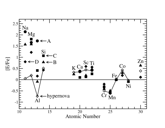
Figure 8: Comparison of the abundance patterns of the low-$A$ elements for HNe and faint SNe. The patterns for HNe are taken to be the same as those for the third source shown in Figure 6 and the data on CS 22885–096 (open diamonds connected by line segments) are shown here as a typical example. The patterns in the anomalous stars (A, B, C, and D) are assumed to represent faint SNe [filled circle: Aoki et al. 2006 (A, HE 1327–2326); filled triangle: Depagne et al. 2002 (B, CS 22949–037); filled square: Aoki et al. 2002 (C, CS 29498–043); filled diamond: Aoki et al. 2007 (D, BS 16934–002)]. Typical observational errors in [E/Fe] are $\sim 0.1$–0.25 dex. Note that the latter patterns are characterized by extremely high abundances of the hydrostatic burning products Na, Mg, and Al relative to the explosive burning products from Si through Zn. Note also that the patterns of the explosive burning products are indistinguishable for HNe and faint SNe.

The three-component model with HNe, $H$, and $L^{*}$ sources describes the available data on nearly all the stars very well. However, there are four exceptional stars that are identified as asterisks A, B, C, and D in Figures 1, 2, 3, and 7a. These stars are not anomalous in terms of Sr and Ba as shown by the above figures. However, Figure 8 shows that their abundance patterns of the low-$A$ elements differ greatly from those for HNe and all the other stars (see discussion of Figure 6 in §3.3). More specifically, while all stars have indistinguishable patterns of the explosive burning products from Si through Zn, these stars have extremely high abundances of the hydrostatic burning products Na, Mg, and Al relative to the explosive burning products. Such anomalous production patterns can be accounted for by faint SNe (e.g., Iwamoto et al. 2005), in which fall-back coupled with a weak explosion would hinder the ejection of the explosive burning products in the inner region much more than that of the hydrostatic burning products in the outer region. Due to the weak explosion, the debris from faint SNe would always be bound to their hosting halos. Mixing with the debris from low-mass and normal SNe to some small extent would preserve the anomalous patterns of the low-$A$ elements and add small amounts of Sr and Ba to the mixture. The stars that formed from this mixture would then appear as the exceptional stars discussed above. Using $Y_{\rm Fe}\sim 4\times 10^{-3}\,M_{\odot}$ and $E_{\rm expl}\sim 4\times 10^{50}$ erg inferred from the light curve of SN 1997D and $Y_{\rm Fe}\sim 2\times 10^{-3}\,M_{\odot}$ and $E_{\rm expl}\sim 6\times 10^{50}$ erg for SN 1999br (see Figure 1 in Tominaga et al. 2007 and references therein), we find that for the corresponding mixing mass (see equations [18]) a single faint SN like these two would result in ${\rm[Fe/H]}\sim-3.5$ (SN 1997D) and $\sim-4$ (SN 1999br) (cf. equation [19]). These [Fe/H] values are close to those of the exceptional stars B (${\rm[Fe/H]}=-3.94$) and C (${\rm[Fe/H]}=-3.70$). This is compatible with a single faint SN giving rise to the anomalous abundance pattern of the low-$A$ elements in each exceptional star.

5 Conclusions

The two-component model of QW07 with the $H$ and $L$ sources provided a good description of the elemental abundances in metal-poor stars of the Galactic halo for $-2.7<{\rm[Fe/H]}\lesssim-1.5$. A key ingredient of that model is the attribution of the elements from Sr through Ag in metal-poor stars to the charged-particle reactions in neutrino-driven winds from nascent neutron stars but not to the $r$-process. However, that model cannot explain the great shortfall in the abundances of Sr, Y, and Zr relative to Fe for stars with ${\rm[Fe/H]}\lesssim-3$. The observations on these three CPR elements require that there be an early source producing Fe but no Sr or heavier elements. It is shown that if such a third source is assumed, then the data can be well explained by an extended three-component model. From considerations of the abundance patterns of the low-$A$ elements (from Na through Zn), it is concluded that this third source is most likely associated with HNe from massive stars of $\sim 25$–$50\,M_{\odot}$ that do not leave behind neutron stars. We here consider the third source to be HNe.

It is shown that the available data on the evolution of [Sr/Fe] with [Ba/Fe], that of [Y/Fe] with [La/Fe], and that of [Zr/Fe] with [Ba/Fe] are well described by the extended model with HNe, $H$ and $L$ sources, which also provides clear constraints on the abundance ratios that should be seen. It is further shown that the abundance patterns of the low-$A$ elements for HNe and the $L$ sources are not distinguishable. Considering that HNe are observed to be ongoing events in the present universe, we are forced to conclude that the $L$ source, which was assumed to have provided $\sim 1/3$ of the solar Fe inventory (the rest attributed to SNe Ia), is in fact a combination of normal SNe (from progenitors of $\sim 12$–$25\,M_{\odot}$), which we define as the $L^{*}$ source, and HNe. The net Fe contributions from HNe are found to be $\sim 3$ times larger than those from normal SNe.

Using the three-component model with HNe, $H$, and $L^{*}$ sources, we obtain a very good quantitative description of essentially all the available data. In particular, this model provides strong constraints on the evolution of [Sr/Fe] with [Ba/Fe] in terms of the allowed domain for these abundance ratios. It gives an equally good description of the data when any CPR element besides Sr (e.g., Y or Zr) or any heavy $r$-element besides Ba (e.g., La) is used. The model is also compatible with the non-$s$-process contributions to the solar abundances of all the CPR elements. The anomalous abundance patterns of the low-$A$ elements observed in a small number of stars appear to fit the description of faint SNe (e.g., Iwamoto et al. 2005), which are a rarer type of events from the same progenitor mass range as HNe but with even weaker explosion energies and smaller Fe yields than normal SNe (e.g., Nomoto et al. 2006). The anomalous abundance patterns observed reflect the fact that faint SNe produce very little of the Fe group elements but an abundant amount of the elements from hydrostatic burning in their outer shells. This gives rise to the extremely high abundances of Na, Mg, and Al relative to Fe observed in the anomalous stars. The quasi-uniform abundance patterns of the elements from Si through Zn in all cases (including the stars with anomalous abundances of Na, Mg, and Al) appear to reflect some robustness in the outcome of explosive burning that may arise from the limited range of conditions required for such nucleosynthesis.

In this paper we used the elemental yield patterns for three prototypical model sources to calculate the abundances of an extensive set of elements (relative to hydrogen) for metal-poor stars with ${\rm[Fe/H]}\lesssim-1.5$. As the yield patterns adopted for the assumed prototypical sources are taken from the data on two template stars, they must represent the results of stellar nucleosynthesis. The full version of the three-component model appears very successful in calculating the abundances of the elements ranging from Na through Pt in stars with ${\rm[Fe/H]}\lesssim-1.5$. In contrast to this phenomenological approach, there are extensive studies of Galactic chemical evolution (GCE) that use the various theoretical results on the absolute yields of metals for different stellar types. These theoretical yields are not calculated from first principles, but are dependent on the parametrization used in the various stellar models. In those GCE studies, the elemental abundances for an individual star are not predicted. Instead, general trends for the elemental abundances are calculated assuming different sources, the rates at which they contribute, and a model of mixing in the ISM for different regions of the Galaxy. These results give a good broad description for typical elemental abundances in the general stellar population at higher metallicities of ${\rm[Fe/H]}>-1.5$. This is a regime in which the observational data are quite convergent with only limited variability. However, as anticipated by Gilroy et al. (1988) and supported by the considerable scatter in the abundances of heavy elements observed in stars with ${\rm[Fe/H]}\lesssim-1.5$, the chemical composition of the ISM in the early Galaxy was extremely inhomogeneous. For ${\rm[Fe/H]}<-2$ there are gross discrepancies between the observations and the smoothed model of GCE. In no case does that model give the elemental abundances for an individual star. It is our view that the simple phenomenological model used here permits a clearer distinction between the different stellar sources contributing to the ISM and the IGM at early times. This model also gives specific testable predictions, which can be used to further check its validity.

In conclusion, we consider that the general three-component model with HNe, $H$, and $L^{*}$ sources provides a quantitative and self-consistent description of nearly all the available data on elemental abundances in stars with ${\rm[Fe/H]}\lesssim-1.5$. Further, HNe may be not only explosions from the first massive stars (i.e., the Population III stars much sought after by many) that provided a very early and variable inventory to the IGM through ejection of enriched gas from small halos, but also are important ongoing contributors to the chemical evolution of the universe.

Appendix A Abundance Ratios in a Well-Mixed ISM

Using equation (1), we calculate the $H$ and $L$ contributions (Sr/H)_⊙,HL to the solar Sr abundance as

$$\left(\frac{\rm Sr}{\rm H}\right)_{\odot,HL}=\left(\frac{\rm Sr}{\rm Eu}\right)_{H}\left(\frac{\rm Eu}{\rm H}\right)_{\odot,H}+\left(\frac{\rm Sr}{\rm Fe}\right)_{L}\left(\frac{\rm Fe}{\rm H}\right)_{\odot,L}.$$ (A1)

As Eu is essentially a pure heavy $r$-element, we take the $H$ contributions to the solar Eu abundance to be ${\rm(Eu/H)}_{\odot,H}\approx{\rm(Eu/H)}_{\odot}$. Allowing for contributions from SNe Ia, we take the $L$ contributions to the solar Fe abundance to be ${\rm(Fe/H)}_{\odot,L}\approx{\rm(Fe/H)}_{\odot}/3$. Using the yield ratios (Sr/Eu)_H and (Sr/Fe)_L given in Table 2, we obtain

$${\rm[Sr/Fe]}_{\rm mix}\equiv\log{\rm(Sr/H)}_{\odot,HL}-\log{\rm(Fe/H)}_{\odot,L}-\log{\rm(Sr/Fe)}_{\odot}=-0.10,$$ (A2)

which we assume to be characteristic of an ISM with well-mixed $H$ and $L$ contributions. Here and throughout the paper (particularly when presenting the data from different observational studies), we have consistently adopted the solar abundances given by Asplund et al. (2005).

The $H$ contributions (Ba/H)_⊙,H to the solar Ba abundance can be calculated as

$$\left(\frac{\rm Ba}{\rm H}\right)_{\odot,H}=\left(\frac{\rm Ba}{\rm Eu}\right)_{H}\left(\frac{\rm Eu}{\rm H}\right)_{\odot,H}\approx\left(\frac{\rm Ba}{\rm Eu}\right)_{H}\left(\frac{\rm Eu}{\rm H}\right)_{\odot}.$$ (A3)

Together with equation (A1), this gives

$${\rm[Sr/Ba]}_{\rm mix}\equiv\log{\rm(Sr/H)}_{\odot,HL}-\log{\rm(Ba/H)}_{\odot,H}-\log{\rm(Sr/Ba)}_{\odot}=0.10$$ (A4)

for an ISM with well-mixed $H$ and $L$ contributions. Combining the above equation with equation (A2) gives

$${\rm[Ba/Fe]}_{\rm mix}={\rm[Sr/Fe]}_{\rm mix}-{\rm[Sr/Ba]}_{\rm mix}=-0.20.$$ (A5)

Other abundance ratios such as [Y/Fe]_mix, [Y/La]_mix, [Zr/Fe]_mix, and [Zr/Ba]_mix for an ISM with well-mixed $H$ and $L$ contributions can be calculated similarly and are given in Table 3.

Table 1: Yield ratios (E/Eu)_H and (E/Fe)_L for the heavy $r$-elements

Element	$\log({\rm E/Eu})_{H}$	$\log({\rm E/Fe})_{L}$	Element	$\log({\rm E/Eu})_{H}$	$\log({\rm E/Fe})_{L}$
Ba	0.97	$-\infty$	Tm	$-0.45$	$-\infty$
La	0.26	$-\infty$	Yb	0.26	$-\infty$
Ce	0.46	$-\infty$	Lu	$-0.50$	$-\infty$
Pr	$-0.03$	$-\infty$	Hf	$-0.13$	$-\infty$
Nd	0.58	$-\infty$	Ta	$-0.88$	$-\infty$
Sm	0.28	$-\infty$	W	$-0.20$	$-\infty$
Gd	0.48	$-\infty$	Re	$-0.27$	$-\infty$
Tb	$-0.22$	$-\infty$	Os	0.82	$-\infty$
Dy	0.56	$-\infty$	Ir	0.85	$-\infty$
Ho	$-0.05$	$-\infty$	Pt	1.14	$-\infty$
Er	0.35	$-\infty$	Au	0.28	$-\infty$

Note. — The (number) yield ratios (E/Eu)_H for the heavy $r$-elements are taken from the corresponding solar $r$-process abundances calculated by Arlandini et al. 1999. The value of $\log{\rm(Ba/Eu)}=0.96$ obtained this way is essentially the same as the value of $\log{\rm(Ba/Eu)}=0.97$ obtained from the data on CS 22892–052 (Sneden et al., 2003). We adopt $\log{\rm(Ba/Eu)}_{H}=0.97$. The yield ratios (E/Fe)${}_{L^{*}}$ for the heavy $r$-elements are the same as (E/Fe)_L.

Table 2: Yield ratios (E/Eu)_H, (E/Ba)_H, (E/Fe)_L, and (E/Fe)${}_{L^{*}}$ for the CPR elements

Element	$\log({\rm E/Eu})_{H}$	$\log({\rm E/Ba})_{H}$	$\log({\rm E/Fe})_{L}$	$\log({\rm E/Fe})_{L^{*}}$
Fe	$-\infty$	$-\infty$	0	0
Eu	0	$-0.97$	$-\infty$	$-\infty$
Ba	0.97	0	$-\infty$	$-\infty$
Sr	1.41	0.44	$-4.85$	$-4.23$
Y	0.53	$-0.44$	$-5.67$	$-5.05$
Zr	1.19	0.22	$-5.02$	$-4.40$
Nb	0.15	$-0.82$	$-6.22$	$-5.60$
Mo	0.55	$-0.42$	$-5.61$	$-4.99$
Ru	1.03	0.06	$-5.60$	$-4.98$
Rh	0.40	$-0.57$	$<-5.94$	$<-5.32$
Pd	0.66	$-0.31$	$-6.10$	$-5.48$
Ag	0.07	$-0.90$	$-6.62$	$-6.00$

Note. — The (number) yield ratios (E/Eu)_H and (E/Ba)_H for the CPR elements are taken from the data on CS 22892–052 (Sneden et al., 2003) and (E/Fe)_L from the data on HD 122563 (Honda et al., 2006). The yield ratios (E/Fe)${}_{L^{*}}$ for the CPR elements are obtained from (E/Fe)_L assuming that 24% of the Fe in the $L$ mixture is from the $L^{*}$ source.

Table 3: Abundance and Yield Ratios Relative to Solar Values

Element	Sr	Y	Zr
${\rm[E/Fe]}_{\rm mix}$	$-0.10$	$-0.24$	0.04
${\rm[E/Ba]}_{\rm mix}$	0.10	$-0.03$	0.24
${\rm[E/La]}_{\rm mix}$	$-0.23$	$-0.36$	$-0.09$
${\rm[E/Ba]}_{H}$	$-0.31$	$-0.48$	$-0.20$
${\rm[E/La]}_{H}$	$-0.64$	$-0.81$	$-0.53$
${\rm[E/Fe]}_{L}$	$-0.32$	$-0.43$	$-0.16$
${\rm[E/Fe]}_{L^{*}}$	0.30	0.19	0.46

Note. — The (number) abundance ratios with subscripts “mix” are calculated for a well-mixed ISM with $H$ and $L$ contributions only (see Appendix A). The (number) yield ratios for the $H$, $L$, and $L^{*}$ sources are labeled with the corresponding subscripts. The $L^{*}$ yield ratios are calculated from the $L$ yield ratios assuming that 24% of the Fe in the $L$ mixture is from the $L^{*}$ source. The solar abundances used are taken from Asplund et al. 2005.

Table 4: Characteristics of HNe, $H$, and $L^{*}$ Sources

Sources	HNe	$H$	$L^{*}$
stellar types	HNe from stars	low-mass SNe from	normal SNe from
	of $\sim 25$–$50\,M_{\odot}$	stars of $\sim 8$–$11\,M_{\odot}$	stars of $\sim 12$–$25\,M_{\odot}$
remnants	black holes	neutron stars	neutron stars
nucleosynthetic	dominant source for	source for CPR elements	source for low-$A$
characteristics	low-$A$ elements	from Sr through Ag	and CPR elements
	from Na through Zn	and only source for heavy
	$f_{\rm Fe,HN}^{\odot}\sim 0.24$	$r$-elements with $A>130$	$f_{{\rm Fe},L^{*}}^{\odot}\sim 0.09$

Table 5: $H$ and $L^{*}$ contributions to the solar inventory of the CPR elements

Element	$\log\epsilon_{\odot}({\rm E})$	$\log\epsilon_{\odot,HL^{*}}({\rm E})$	$f_{{\rm E},HL^{*}}^{\odot}$	$(1-f_{{\rm E},s}^{\odot})_{\rm Arlandini}$	$(1-f_{{\rm E},s}^{\odot})_{\rm Travaglio}$
	(1)	(2)	(3)	(4)	(5)
Sr	2.92	2.34	0.26	0.15	0.20
Y	2.21	1.50	0.19	0.08	0.26
Zr	2.59	2.15	0.36	0.17	0.33
Nb	1.42	1.01	0.39	0.15	0.31
Mo	1.92	1.54	0.42	0.50	0.61
Ru	1.84	1.77	0.85	0.68	0.76
Rh	1.12	$>0.92$	$>0.63$	0.86	0.90
Pd	1.69	1.35	0.46	0.54	0.64
Ag	0.94	0.79	0.71	0.80	0.91

Note. — Column 1 gives the solar abundances of the CPR elements from Asplund et al. 2005, col. 2 gives the $H$ and $L^{*}$ contributions to the solar inventory of these elements as calculated from the three-component model using the yield ratios given in Table 2, col. 3 gives the fraction of the solar inventory provided by the $H$ and $L^{*}$ sources as calculated from cols. 1 and 2 using $\log f_{{\rm E},HL^{*}}^{\odot}=\log\epsilon_{\odot,HL^{*}}({\rm E})-\log\epsilon_{\odot}({\rm E})$, and cols. 4 and 5 give the fraction contributed by processes other than the $s$-process using the $s$-fraction $f_{{\rm E},s}^{\odot}$ calculated by Arlandini et al. 1999 and Travaglio et al. 2004, respectively. As the exact value of (Rh/Fe)${}_{L^{*}}$ is unknown (see Table 2), we calculate only the $H$ contribution to Rh and give the corresponding lower limits in cols. 2 and 3. Note that the fraction $f_{{\rm E},HL^{*}}^{\odot}$ contributed by the $H$ and $L^{*}$ sources is in approximate agreement with the fraction $1-f_{{\rm E},s}^{\odot}$ attributed to non-$s$-process sources by Arlandini et al. 1999 and Travaglio et al. 2004 for the elements Mo, Ru, Rh, Pd, and Ag with small to moderate $s$-process contributions. For the elements Sr, Y, Zr, and Nb with large $s$-process contributions, the fraction $f_{{\rm E},HL^{*}}^{\odot}$ is a factor of $\approx 2$ larger than the fraction $1-f_{{\rm E},s}^{\odot}$ estimated by Arlandini et al. 1999 but in good agreement with that estimated by Travaglio et al. 2004, who carried out a detailed study of Galactic chemical evolution for the $s$-process contributions to these elements. The problem in estimating the non-$s$-process contributions to these elements has been discussed by Qian & Wasserburg 2001 and Travaglio et al. 2004. It appears that the increase in the non-$s$-process contributions found again here is justified in terms of both abundance data on metal-poor stars and uncertainties in modeling the $s$-process contributions.

References

- Abel et al. (2002) Abel, T., Bryan, G. L., & Norman, M. L. 2002, Science, 295, 93
- Anders & Grevesse (1989) Anders, E., Grevesse, N. 1989, Geochim. Cosmochim. Acta, 53, 197
- Aoki et al. (2005) Aoki, W., et al. 2005, ApJ, 632, 611
- Aoki et al. (2006) Aoki, W., et al. 2006, ApJ, 639, 897
- Aoki et al. (2007) Aoki, W., et al. 2007, ApJ, 660, 747
- Aoki et al. (2002) Aoki, W., Norris, J. E., Ryan, S. G., Beers, T. C., & Ando, H. 2002, ApJ, 576, L141
- Arlandini et al. (1999) Arlandini, C., et al. 1999, ApJ, 525, 886
- Asplund et al. (2005) Asplund, M., Grevesse, N., & Sauval, A. J. 2005, in ASP Conf. Ser. 336, Cosmic Abundances as Records of Stellar Evolution and Nucleosynthesis, ed. T. G. Barnes III & F. N. Bash (San Francisco: ASP), 25
- Barkana & Loeb (2001) Barkana, R., & Loeb, A. 2001, Phys. Rep., 349, 125
- Barklem et al. (2005) Barklem, P. S., et al. 2005, A&A, 439, 129
- Bromm & Larson (2004) Bromm, V., & Larson, R. B. 2004, ARA&A, 42, 79
- Cappellaro et al. (1999) Cappellaro, E., Evans, R., & Turatto, M. 1999, A&A, 351, 459
- Cayrel et al. (2004) Cayrel, R., et al. 2004, A&A, 416, 1117
- Chieffi & Limongi (2004) Chieffi, A., & Limongi, M. 2004, ApJ, 608, 405
- Christlieb et al. (2002) Christlieb, N., et al. 2002, Nature, 419, 904
- Christlieb et al. (2004) Christlieb, N., et al. 2004, ApJ, 603, 708
- Cohen et al. (2007) Cohen, J. G., et al. 2007, ApJ, 659, L161
- Cohen et al. (2008) Cohen, J. G., et al. 2008, ApJ, 672, 320
- Cowan et al. (2002) Cowan, J. J., et al. 2002, ApJ, 572, 861
- Depagne et al. (2002) Depagne, E., et al. 2002, A&A, 390, 187
- Duncan et al. (1986) Duncan, R. C., Shapiro, S. L., & Wasserman, I. 1986, ApJ, 309, 141
- François et al. (2007) François, P., et al. 2007, A&A, 476, 935
- Frebel et al. (2007) Frebel, A., et al. 2005, Nature, 434, 871
- Frebel et al. (2007) Frebel, A., et al. 2007, ApJ, 658, 534
- Fulbright et al. (2004) Fulbright, J. P., Rich, R. M., & Castro, S. 2004, ApJ, 612, 447
- Galama et al. (1998) Galama, T. J., et al. 1998, Nature, 395, 670
- Gao et al. (2007) Gao, L., et al. 2007, MNRAS, 378, 449
- Gilroy et al. (1988) Gilroy, K. K., Sneden, C., Pilachowski, C. A., & Cowan, J. J. 1988, ApJ, 327, 298
- Greif et al. (2007) Greif, T. H., Johnson, J. L., Bromm, V., & Klessen, R. S. 2007, ApJ, 670, 1
- Heger & Woosley (2002) Heger, A., & Woosley, S. E. 2002, ApJ, 567, 532
- Hill et al. (2002) Hill, V., et al. 2002, A&A, 387, 560
- Hoffman et al. (1997) Hoffman, R. D., Woosley, S. E., & Qian, Y.-Z. 1997, ApJ, 482, 951
- Honda et al. (2004) Honda, S., et al. 2004, ApJ, 607, 474
- Honda et al. (2006) Honda, S., Aoki, W., Ishimaru, Y., Wanajo, S., & Ryan, S. G. 2006, ApJ, 643, 1180
- Iwamoto et al. (1998) Iwamoto, K., et al. 1998, Nature, 395, 672
- Iwamoto et al. (2005) Iwamoto, N., Umeda, H., Tominaga, N., Nomoto, K., & Maeda, K. 2005, Science, 309, 451
- Janka et al. (2007) Janka, H.-T., Müller, B., Kitaura, F. S., & Buras, R. 2007, preprint (arXiv: 0712.4237 [astro-ph])
- Johnson (2002) Johnson, J. A. 2002, ApJS, 139, 219
- Johnson & Bolte (2002) Johnson, J. A., & Bolte, M. 2002, ApJ, 579, 616
- Kitayama & Yoshida (2005) Kitayama, T., & Yoshida, N. 2005, ApJ, 630, 675
- McWilliam et al. (1995) McWilliam, A., Preston, G. W., Sneden, C., & Searle, L. 1995, AJ, 109, 2757
- Meyer et al. (1992) Meyer, B. S., Mathews, G. J., Howard, W. M., Woosley, S. E., & Hoffman, R. D. 1992, ApJ, 399, 656
- Ning et al. (2007) Ning, H., Qian, Y.-Z., & Meyer, B. S. 2007, ApJ, 667, L159
- Nomoto (1984) Nomoto, K. 1984, ApJ, 277, 791
- Nomoto (1987) Nomoto, K. 1987, ApJ, 322, 206
- Nomoto et al. (2006) Nomoto, K., Tominaga, N., Umeda, H., Kobayashi, C., & Maeda, K. 2006, Nucl. Phys. A, 777, 424
- Norris et al. (2001) Norris, J. E., Ryan, S. G., & Beers, T. C. 2001, ApJ, 561, 1034
- Norris et al. (2007) Norris, J. E., et al. 2007, ApJ, 670, 774
- O’Shea & Norman (2007) O’Shea, B. W., & Norman, M. L. 2007, ApJ, 654, 66
- Qian et al. (2002) Qian, Y.-Z., Sargent, W. L. W., & Wasserburg, G. J. 2002, ApJ, 569, L61
- Qian & Wasserburg (2001) Qian, Y.-Z., & Wasserburg, G. J. 2001, ApJ, 559, 925
- Qian & Wasserburg (2002) Qian, Y.-Z., & Wasserburg, G. J. 2002, ApJ, 567, 515
- Qian & Wasserburg (2004) Qian, Y.-Z., & Wasserburg, G. J. 2004, ApJ, 612, 615
- Qian & Wasserburg (2007) Qian, Y.-Z., & Wasserburg, G. J. 2007, Phys. Rep., 442, 237 (QW07)
- Qian & Woosley (1996) Qian, Y.-Z., & Woosley, S. E. 1996, ApJ, 471, 331
- Simmerer et al. (2004) Simmerer, J., et al. 2004, ApJ, 617, 1091
- Sneden et al. (2003) Sneden, C., et al. 2003, ApJ, 591, 936
- Takahashi et al. (1994) Takahashi, K., Witti, J., & Janka, H.-T. 1994, A&A, 286, 857
- Thielemann et al. (1996) Thielemann, F.-K., Nomoto, K., & Hashimoto, M. 1996, ApJ, 460, 408
- Thornton et al. (1998) Thornton, K., Gaudlitz, M., Janka, H.-Th., & Steinmetz, M. 1998, ApJ, 500, 95
- Tominaga et al. (2007) Tominaga, N., Umeda, H., & Nomoto, K. 2007, ApJ, 660, 516
- Travaglio et al. (2004) Travaglio, C., et al. 2004, ApJ, 601,864
- Turatto et al. (1998) Turatto, M., et al. 1998, ApJ, 498, L129
- Wasserburg et al. (1996) Wasserburg, G. J., Busso, M., & Gallino, R. 1996, ApJ, 466, L109
- Woosley & Hoffman (1992) Woosley, S. E., & Hoffman, R. D. 1992, ApJ, 395, 202
- Woosley & Weaver (1995) Woosley, S. E., & Weaver, T. A. 1995, ApJS, 101, 181
- Woosley et al. (1994) Woosley, S. E., Wilson, J. R., Mathews, G. J., Hoffman, R. D., & Meyer, B. S. 1994, ApJ, 433, 229
- Yoshida et al. (2006) Yoshida, N., Omukai, K., Hernquist, L., & Abel, T. 2006, ApJ, 652, 6