The Ultimatum Game in Complex Networks

Abstract

We address the problem of how cooperative (altruistic-like) behavior arises in natural and social systems by analyzing an ultimatum game in complex networks. Specifically, three types of players are considered: (a) empathetic, whose aspiration level and offer are equal, (b) pragmatic, who do not distinguish between the different roles and aim to obtain the same benefit, and (c) agents whose aspiration level and offer are independent. We analyze the asymptotic behavior of pure populations on different topologies using two kinds of strategic update rules. Natural selection, which relies on replicator dynamics, and Social Penalty, inspired in the Bak-Sneppen dynamics, in which players are subjected to a social selection rule penalizing not only the less fitted individuals, but also their first neighbors. We discuss the emergence of fairness in the different settings and network topologies.

Keywords: Network dynamics, Collective phenomena in economic and social systems

1 Introduction

Human cooperation has been the focus of intense debate within the theoretical framework of evolutionary theories since long time ago [1, 2]. In particular, altruistic behavior, in which individuals perform costly acts for themselves to confer benefits to the rest of the population, has often been identified as a key mechanism for cooperation. A number of theoretical approaches have been developed to explain the emergence of human altruism. Kin selection theory [3] accounts for situations in which it pays off (inclusive fitness) to help relatives that share some fraction of the genetic pool. In the absence of such kin relationships, repeated interactions have also been shown to lead to cooperation, as well as different kinds of reciprocity mechanisms [2, 4, 5, 6]. Recently, a series of behavioral experiments in which interactions are anonymous and one-shot have shown that humans can punish non-cooperators (altruistic punishment) and reward those individuals who cooperate (altruistic rewarding) [2, 7, 8, 9, 10]. This so-called strong reciprocity can actually explain the observed cooperative behavior in terms of group and cultural selection. However, standard evolutionary game theory is still far from explaining how cooperation may arise from selection at the individual level. Recent steps in this direction [11] have contributed to fill this gap, although a general theoretical framework is still needed.

On the other hand, recent discoveries on the architecture of biological, technological and social systems have shown that the structure of these systems has important consequences on their dynamical behavior [12, 13]. In particular, the dynamical features observed in heterogeneous, scale-free networks, are radically different from those in homogenous networks. This difference is due to the presence of highly connected nodes. For instance, in epidemic spreading, the hubs are very efficient in propagating the disease [14, 15], up to the point that in heterogeneous networks the epidemic threshold vanishes in the limit of infinite system size. In some other processes, the hubs play the opposite role. An example is rumor spreading [16], where a larger number of ”infected” nodes is obtained in homogeneous networks. Finally, there are situations where hubs play a more subtle role. This is the case of synchronization phenomena [17]. In many systems, scale-free (SF) networks exhibit a smaller threshold for the onset of synchronization. Nonetheless, the stability of the fully synchronized state is less robust in SF networks than in random graphs.

Motivated by the aforementioned results, studies of evolutionary game theory models on hetereogenous networks have attracted much attention in the last years [6, 18, 19, 20, 21, 22, 23, 24]. Issues such as the influence of the social structure in cooperative behavior, as well as the role of the highly connected nodes have been mainly explored in the context of the Prisoner’s Dilemma [19, 20, 21, 23]. The results obtained point out that SF networks are best suited to support cooperation and that hubs play a fundamental role in spreading cooperation through a positive feedback mechanism, even when it is expensive. The same kind of results have been recently reported for public good games [25].

Here we focus on the Ultimatum Game (UG), another kind of game extensively used to model altruistic behavior [26], but not adequately explored in the context of complex networks, though spatial effects have been considered to some extent (see for instance [27] for the UG model on regular 1D and 2D lattices). The standard UG considers that two players bargain to divide a fixed reward between them. Suppose that one of these players acts as proposer offering a division of the reward. The other, henceforth called respondent, can accept or reject this proposal, but cannot counteroffer. If the respondent accepts, the reward is divided as agreed, otherwise both receive nothing. For a one-shot game played anonymously, the rational solution (subgame perfect Nash equilibrium solution) is that in which the proposer would offer the smallest possible share and the respondent would accept it. However, plenty of experimental results point out that the rational solution is not what actually happens. For instance in the social context, it has been shown that the mean offer is usually between $40\%$ and $50\%$ and that offers below $20\%$ of the reward are often rejected [28, 29]. This has been interpreted as an example of altruistic punishment [7, 10], i.e., the tendence to impose sanctions on unfair individuals with a cost for the punisher. However, costly punishment has been proven [30] to be maladaptive (winners do not punish) which leaves open the question on how this trait has evolved.

We implement here two kinds of evolution rules (see below): one is fitness-dependent and is based on a pairwise comparison, in the spirit of [21, 23], and the second one is inspired in the Bak-Sneppen model [31, 32, 33] of punctuated equilibrium. Summing up, in the present work, we study an UG model on Erdös-Rényi and Scale-free networks with three different kinds of settings of the parameters characterizing the players. The asymptotic evolutionary states reached following the two update rules cited above are analyzed and compared in the three different frameworks.

2 The model

In our model we consider $N$ individuals associated to the nodes of a graph. The graph topologies we will study are of two different kinds: Erdös-Rényi (ER) and Scale-free (SF) networks. An ER network is characterized by a degree distribution that decays exponentially fast for large $k$, while in a SF network the degree distribution follows a power-law of the form $P_{k}\sim k^{-\gamma}$. We consider SF networks with $\gamma\approx 3$ [34]. Therefore, while in ER networks the number of contacts shared by individuals shows a finite variance, in SF networks we find nodes, usually referred to as hubs, that interact with a large fraction of the population.

2.1 Playing the Ultimatum Game

The individuals on the nodes of the aforementioned networks play the Ultimatum Game (UG). At each time step, each individual plays a round robin of the game with all his neighbors, as dictated by the graph. In each round, individuals play the UG twice with each neighbor, both as proposers and as respondents. The reward to divide in each of these two games is equal to $1$. An individual $i$ ($i=1,...,N$) is characterized by two parameters: $p_{i}$, $q_{i}$ $\in[0,1]$. When $i$ acts as proposer it offers a division $p_{i}$ of the reward, so that the respondent will earn $p_{i}$ if the proposal is accepted. Instead, when agent $i$ plays as respondent, it will accept only offers larger than its acceptance threshold $q_{i}$. Therefore, when two individuals ($i,j$) bargain, their payoffs, $\Pi_{i}$ and $\Pi_{j}$, evolve according to the following rules:

• Player $i$ offers the amount $p_{i}$ to $j$. If $p_{i}\geq q_{j}$, the offer is accepted and the payoff of $i$ and $j$ are incremented by $\Delta\Pi_{ij}^{O}=(1-p_{i})$ and $\Delta\Pi^{R}_{ji}=p_{i}$ respectively. Conversely, if $p_{i}<q_{j}$, agreement is not possible and both players get nothing and their payoffs remain the same, $\Delta\Pi_{ij}^{O}=\Delta\Pi^{R}_{ji}=0$.

• When player $i$ is the respondent, the same rules apply. Therefore, upon agreement ($p_{j}>q_{i}$), players $i$ and $j$ increase their payoffs by $\Delta\Pi^{R}_{ij}=p_{j}$ and $\Delta\Pi^{O}_{ji}=(1-p_{j})$ respectively.

The final payoffs of a node $i$ after playing with all its neighbors is

$$\Pi_{i}=\sum_{l\in\Gamma_{i}}(\Delta\Pi_{il}^{O}+\Delta\Pi_{il}^{R})\;,$$ (1)

where $\Gamma_{i}$ denotes the set of $i$’s neighbors.

In the following, we will study three different settings for the values of the parameters $p_{i}$ and $q_{i}$:

1. For each agent $i$, $p_{i}=q_{i}$ [35]. This is usually called a fair or empathetic setting since each agent offers the same reward it is disposed to accept;

2. For each agent $i$, $p_{i}=1-q_{i}$ [36]. This is a role-ignoring or pragmatic setting since each agent wants to get the same reward both as respondent and as proposer;

3. The values of $p_{i}$ and $q_{i}$ are independent for each agent.

The second choice B stands for a situation in which players do not differentiate between roles (role-ignoring agents). In other words, regardless of whether they act as proposers or responders, they are determined to obtain a fixed quantity from each interaction, so that $q_{i}=1-p_{i}$ [36]. This situation is in contrast with the case of an empathetic or fair and role-distinguishing setting A, according to which individuals do distinguish among roles. In this case the threshold of acceptance is set equal to the one for proposals ($q_{i}=p_{i}$), so as to get half of the total stake on average. Finally, in the third setting C the quantity offered and the threshold of acceptance are completely independent as in the original formulation of the UG.

Note, that in both cases A and B, the corresponding relations $p(q)$ allow to obtain simple rules for the conclusion of a deal between two players. Given that the offer $p_{i}$ proposed by player $i$ is accepted by $j$ only if $p_{i}\geq q_{j}$ we have the two following scenarios:

1. Case $p=q$: if $p_{i}\neq p_{j}$ $i$ and $j$ always conclude a deal, but only in one of the two directions. In particular, the accepted offer is the largest one: $\max\{p_{i},p_{j}\}$. If for example $p_{i}>p_{j}$, the payoffs are incremented by:

   $$\Delta\Pi_{ij} = \Delta\Pi^{O}_{ij}=1-p_{i}\;,$$ (2)

   $$\Delta\Pi_{ji} = \Delta\Pi^{R}_{ji}=p_{i}\;.$$ (3)

   If $p_{i}=p_{j}$ the deal is concluded in both directions and their payoffs are incremented in $\Delta\Pi_{ij}=\Delta\Pi_{ji}=1$, which is the maximum possible reward after the interaction between two players of type A.

2. Case $p=1-q$: both players $i$ and $j$ will obtain reward both as proposers and respondents if the condition $p_{i}+p_{j}\geq 1$ is verified. In this case, their payoffs are incremented by

   $$\Delta\Pi_{ij} = \Delta\Pi^{O}_{ij}+\Delta\Pi^{R}_{ij}=(1-p_{i})+p_{j}\;,$$ (4)

   $$\Delta\Pi_{ji} = \Delta\Pi^{O}_{ji}+\Delta\Pi^{R}_{ji}=(1-p_{j})+p_{i}\;.$$ (5)

   When $p_{i}+p_{j}<1$ no payoff is obtained in the round.

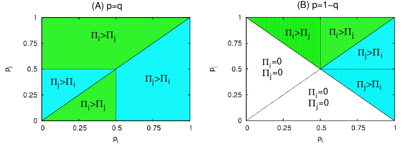
We illustrate the different ordering in payoffs for the two type of players in Figure 1.

2.2 Updating the strategies

Once a player has bargained with all its neighbors, the accumulated payoff drives the update of their strategies. This update process takes place at the individual level, in the same spirit of [11], and follows two different schemes:

• Natural selection: In this framework, originally introduced in [37, 38], each player $i$ in the network selects at random one neighbor $j$ and compares its payoff $\Pi_{i}$ with the one of $j$, $\Pi_{j}$. If $\Pi_{j}>\Pi_{i}$, player $i$ adopts the strategy of $j$, ($p_{j}$, $q_{j}$), for the next round of the UG with a probability proportional to the payoff difference:

  $$P_{ij}=\frac{\Pi_{j}-\Pi_{i}}{2\max\{k_{i},k_{j}\}}\;.$$ (6)

  where $k_{i}$ and $k_{j}$ are the degrees of $i$ and $j$ respectively. Instead, if $\Pi_{i}\leq\Pi_{j}$, $i$ keeps his strategy for the following round.

• Social penalty: The player with lowest payoff in the whole population together with its neighbors, no matter how wealthy they are, are removed. These agents are replaced in their nodes by new players with random strategies (so that they only inherit their contacts).

In the case of Natural selection, there is a pairwise comparison thanks to which fittest strategies are replicated with a rate proportional to their success, with the result of eventually spreading over the whole population [21]. As we will discuss, these dominant strategies might not promote the welfare of the population since it acts at a local level. On the contrary, Social penalty acts at the global level; the removal of all the neighbors of the least-fitted agent is a catastrophic effect triggered by his extinction (see [31] for a discussion on the evolutionary justification of this updating rule) and not related to individuals’ fitness but to the network of interactions. This undiscriminating (and likely unfair) social penalty is imposed on those agents that in the community are responsible for the low fitness of the dying agent; thus it is quite different from the current notion of (altruistic) punishment commented above. With this evolutionary rule, a player, in order to survive, has to take care not only of his payoff, but also of the neighbors’ one: if an individual exploits its neighborhood so that it takes a large stake of the total reward, it would risk to be dropped out of the game as a result of one of its neighbors being that with the lowest payoff in the population of players. In both the Social penalty and Natural selection contexts, after the implementation of the update rule, the payoffs of the agents are reset to zero. This means that players have no memory of the previous round payoffs, although they keep their strategies; consequently it is a one-shot game and no mechanism of reputation has been explicitly introduced [36].

In the following, we will analyze the scenarios concerning these two updating rules in ER and SF topologies for the three strategic settings A, B and C introduced above.

Figure 1: The figures show the partition of the strategies space of a two UG players ($i$ and $j$) into different regions. Each of these regions is labelled according to the payoffs ordering: green areas correspond to the case $\Pi_{i}>\Pi_{j}$, blue areas to $\Pi_{j}>\Pi_{i}$. The regions in white correspond to the case of a zero reward for both players $\Pi_{i}=\Pi_{j}=0$. (See text for the details).

3 The Ultimatum game with Natural selection

The behavior of players of type $A$ (empathetic) and $B$ (pragmatic) can be easily predicted in a well-mixed population when a replicator-like dynamics is at work. Because of this, in the following two subsections we will first discuss the evolution of the game in a well-mixed population and then compare it with the numerical results obtained for homogeneous and heterogeneous networks.

3.1 Networks of type A players ($p=q$)

As mentioned above, in a round robin between two empathetic ($q=p$) players $i$ and $j$ the largest offer, say $p_{i}$, is always accepted by the player offering less, hence $j$, and the payoff obtained will be those of eqs. (2) and (3). In the case of $p_{i}>p_{j}$, two situations are possible: (i) $p_{i}>0.5$, so that $\Pi_{j}>\Pi_{i}$ and (ii) $p_{i}<0.5$, yielding $\Pi_{i}>\Pi_{j}$ (see Figure 1.a).

In the case of the dynamics of a well-mixed population where all the individuals interact with the rest of the players, given the distribution $D(p)$ of offers in the population one finds that the payoff received by strategist offering $x$ is $\Pi(x)=G(x)+\langle p\rangle-H(x)$ where:

$$G(x) = (1-x)\int_{0}^{x}D(p){\mbox{d}}p\;,$$ (7)

$$H(x) = \int_{0}^{x}pD(p){\mbox{d}}p\;,$$ (8)

$$\langle p\rangle = \int_{0}^{1}pD(p){\mbox{d}}p\;.$$ (9)

In the case of replicator dynamics, the increase or decrease of the fraction of players using strategy $x$ is determined by $\Pi(x)-\langle\Pi\rangle$, being $\langle\Pi\rangle$ the average payoff in the population. For a uniform distribution $D(p)=1$ one obtains $\Pi(x)-\langle\Pi\rangle=x-3x^{2}/2$ and one concludes that from an initial uniform distribution the highest values of $p$ will soon become extinct, and the highest increase in frequency will occur for values centered at $x=1/3$. Once most of players use offers below $1/2$, the selective advantage is for players with higher $p$ (below $1/2$). Thus, one expects that the values of $p$ will concentrate at $p=1/2$. This two stage dynamics will be obtained also in the context of complex networks.

(a) ER $p=q$

(b) SF $p=q$

(c) ER $p=1-q$

(d) SF $p=1-q$

Figure 2: Distribution of offers $D(p)$ for ER and SF networks in the cases $p=q$ [(a) and (b)] and $p=1-q$ [(c) and (d)] when a Replicator-like update rule, eq. (6), is at work.

We show the results obtained with this dynamics on top of ER and SF networks. In both cases the networks have $N=10^{4}$ nodes and average degree $\langle k\rangle=4$. The evolutionary dynamics starts assigning to each individual of the population a random offer $p_{i}$ (and thus $p_{i}=q_{i}$) uniformly distributed in the interval $[0,1]$. Then, we follow the system evolution for a number of time steps until a stationary regime is reached. The results presented are averaged over at least $10^{3}$ realizations of both the underlying network and the initial conditions.

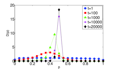
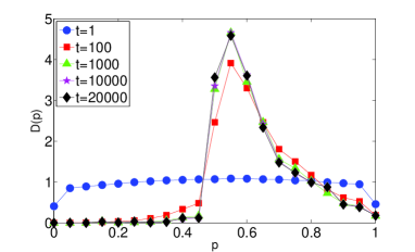
Figures 2.a and 2.b show the time evolution of the distribution of offers $D(p)$ in the population for both ER and SF networks. It is evident that for ER networks the distribution $D(p)$ after $t=2\cdot 10^{4}$ generations shows qualitatively the shape predicted using the well-mixed assumption. Moreover, the two-stage evolution explained above is also confirmed by looking at the time evolution of $D(p)$. From $t=1$ to $t=10^{2}$ the strategists with $p>0.5$ are removed and invaded by those players with low values of $p$. After this initial stage, the flow of strategies goes from low values of $p$ towards $p=0.5$, reaching the final distribution peaked at $p\simeq 0.5$ with a fast decaying tail at $p<0.5$.

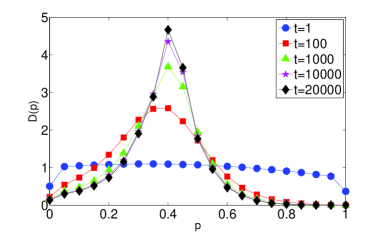
In the case of SF networks the asymptotic distribution of offers $D(p)$ becomes broader with respect to ER graphs. Remarkably the two-stage process is also observed since most of strategies with large values of $p$ are removed in the first time steps. On the other hand, at variance with ER networks, some strategies with $p>0.5$ survive in the final population. This result is the consequence of having individuals, named hubs, with large degree $k_{h}>\langle k\rangle$. The analysis of a “coarse grained” picture of degree-homogeneous population of size $N$ and mean degree $\langle k\rangle$ with an individual connected to a large number, $k_{h}$, of individuals of this population can help us to understand what takes place for SF networks. Suppose that the population has reached its internal equilibrium and therefore $p_{i}\simeq 0.5$ for all its members. In the case $p_{h}<0.5$ (selfish hubs), a hub obtains a payoff $\Pi_{h}=k_{h}/2$ while the members of the population connected to the hub obtains $\Pi_{i}=\langle k\rangle+1/2$. In this case, the hub survives (i.e. satisfies $\Pi_{h}\geq\Pi_{i}$) for every value $p_{h}<0.5$ provided that $k_{h}\geq 2\langle k\rangle+1$, a condition that is easily verified in SF for large degree nodes. On the other hand, if $p_{h}>0.5$ (generous hubs) we have $\Pi_{h}=k_{h}(1-p_{h})$ and on average $\langle\Pi\rangle=\langle k\rangle+p_{h}$ for the individuals connected to the hub. Therefore, if generous hubs are to survive in the system they cannot offer more than $p_{h}\leq(1-\langle k\rangle/k_{h})$. This maximum offer tend to $1$ as $k_{h}$ grows, thus explaining the existence of a tail for $p>0.5$ in the distribution $D(p)$ of SF networks. In both cases, the strategy of hubs is eventually replicated by the rest of the population and after enough generations the payoff of the hub is $\Pi_{h}=k_{h}$ while $\langle\Pi\rangle=\langle k\rangle$ for its neighbors. Hence, heterogeneity can help the fixation of altruistic behavior in nodes provided they have a large number of contacts to obtain enough payoff.

3.2 Networks of type B players ($p=1-q$)

Let’s now focus on the case B. In this context, two players $i$ and $j$ conclude a deal only when $p_{i}+p_{j}\geq 1$. If this condition holds, the consensus is automatically reached in both directions, and the payoffs of the players are those specified in eqs. (4) and (5). The line (see Figure 1.b) $p_{i}=1-p_{j}$ delimitates the area of unsuccessful strategies (below the line), since no payoff is obtained, from that of the successful ones (above the line). This latter region can be further divided into two triangular areas: that of $p_{i}>p_{j}$, yielding $\Pi_{j}>\Pi_{i}$, and the one of $p_{j}>p_{i}$, giving $\Pi_{i}>\Pi_{j}$. Obviously, the border between the two regions is specified by $p_{i}=p_{j}$ (see Figure 1.b).

For a well mixed with a distribution density of offers $D(p)$, the payoff of strategist $x$ is $\Pi(x)=G^{\prime}(x)+H^{\prime}(x)$ where:

$$G^{\prime}(x) = (1-x)\int_{1-x}^{1}D(p){\mbox{d}}p\;,$$ (10)

$$H^{\prime}(x) = \int_{1-x}^{1}pD(p){\mbox{d}}p\;.$$ (11)

For an initial uniform density $D(p)=1$, one obtains $\Pi(x)-\langle\Pi\rangle=-3x^{2}/2+2x-1/2$ whose graph is mirror-symmetric around $x=1/2$ of the one obtained for type A players. Thus, one expects a fast extinction of lowest offers and an initially higher growth of offers around $2/3$. Once offers below $1/2$ become extinct, one easily realizes that for any arbitrary corresponding density ($D(p)=0$ for $p<1/2$), $\Pi(x)-\langle\Pi\rangle=\langle p\rangle-x$ so that the selective advantage is for offers as close to $p=1/2$ as possible. Therefore one expects a progressive displacement to $p=1/2$ values of the maximum of the evolving density.

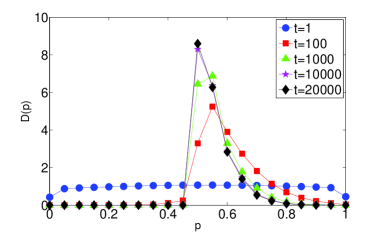
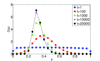
When performing simulations of B players on ER networks, similarly to what happens for A players (see 3.1), the asymptotic distribution of offers agrees with the well-mixed predictions, as Figure 2.c confirms. Here the distribution at $t=2\cdot 10^{4}$ shows a peak at $p=0.5$ and a fast decaying tail for $p>0.5$. This tail proves that strategies moves towards $p=0.5$ from the right, i.e. from the successful region of the $N$-dimensional space. Remarkably, the strategies with $p<0.5$ are totally removed from the population already at $t=100$.

The distribution of offers $D(p)$ in SF networks, Figure 2.d, shows also a peak around $p=0.5$ but with a tail for $p>0.5$ decreasing slower than in ER networks. This behavior can be explained again with the presence of highly connected players. Following the same argument used for A players, a hub with an offer $p_{h}>0.5$, connected to a large number $k_{h}$ of individuals with $p\simeq 0.5$ and mean degree $\langle k\rangle$, obtains a payoff $\Pi_{h}=k_{h}(3/2-p_{h})$ whereas for the individuals connected to the hub on average $\langle\Pi\rangle=\langle k\rangle+p_{h}+1/2$. In this setting, the hub will survive and spread its strategy provided $p_{h}\leq(3/2-\langle k\rangle/k_{h})$. Therefore offers of hubs can also reach $p=1$ as observed in the distribution $D(p)$ for SF networks. Similarly as in the case of type A players, once the hub’s neighbors have imitated its strategy the payoffs of the hub and its neighbors are $\Pi_{h}=k_{h}$ while $\langle\Pi\rangle=\langle k\rangle$ respectively. In the case $p_{h}<0.5$, since the condition $p_{h}+p_{i}\geq 1$ is no longer verified, the region with $p<0.5$ keeps on being forbidden, in agreement with the sharp decay of $D(p)$ in Figure 2.d.

Interestingly, at variance with the case of type A players in which the unsuccessful strategies of the well-mixed case ($p>0.5$) are allowed to the high degree nodes of SF networks, in the case of B players the unsuccessful region of strategies of the well-mixed limit ($p<0.5$) is always empty, regardless of the underlying topology of interactions.

(a) ER $(p,q)$

(b) SF $(p,q)$

(c) ER $(p,q)$

(d) SF $(p,q)$

Figure 3: The distributions of offers $D(p)$ [(a) and (b)] and of acceptance thresholds $D(q)$ [(c) and (d)] for ER [(a) and (c)] and SF [(b) and (d)] networks when a Replicator-like update rule, eq. (6), is at work.

3.3 Networks of type C players (independent $p$ and $q$)

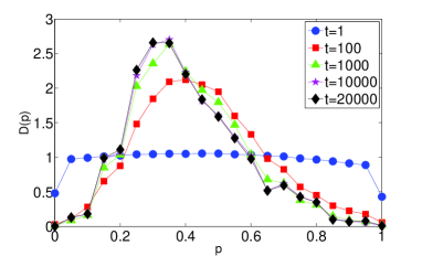
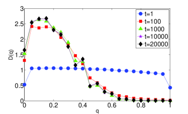
Finally, we explore the situation according to which players are allowed to choose their offers $p$ and acceptance thresholds $q$ independently. In Figures 3.a and 3.b we plot the distribution of offers $D(p)$ for ER and SF networks respectively. Remarkably the two distributions show a maximum around $p\simeq 0.3$, pointing out that offers are quite poor in this third setting. In the case of ER, nearly all the offers are concentrated around the maximum and time evolution shows that large offers dissapear first from the population, similarly to the case of players A on ER networks. For SF networks $D(p)$ is remarkably broader having nonzero values for the entire range of $p\in[0,1]$. Therefore, only in SF networks we observe some degree of altruistic behavior, although the probability of finding offers with $p>0.5$ is lower than that for $p<0.5$.

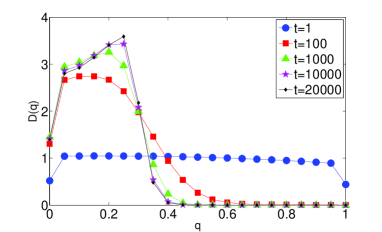
Turning the attention to the distribution of acceptance thresholds $D(q)$ (Figures 3.c and 3.d) we observe that both networks present quite similar behaviors since in both, players accept low offers although they are still far from a fully rational behavior ($q=0$). In particular, for ER networks any offer above $0.4$ will be accepted. In the case of SF networks this global threshold is slightly larger although the probability of finding acceptance thresholds with $q>0.5$ is extremely low. Interestingly, in both distributions we find that the probability of finding players with $q=0$ is nonzero.

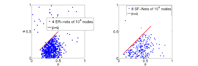
We have also checked what is the correlation, if any, between the values of $p$ and $q$ chosen by the players in order to unveil whether there is a natural tendency towards one of the two settings A ($p=q$) or B ($p=1-q$). In Figure 4 the two scatter plots are realized by representing the set of individual strategies $\{(p_{i},q_{i})\}$ observed in the asymptotic state for several realizations of the UG dynamics. In both ER (Figure 4.a) and SF (Figure 4.b) networks one can observe that $p_{i}\geq q_{i}$ holds for most of the populations. This tendency clearly indicates that players are neither of type A nor of type B, although, given the low value of the average offer $p\simeq 0.3$, their behavior resemble more that of players of type A.

Figure 4: Scatter plot of the individual stragies $(p_{i},q_{i})$ in the asymtotic regime for ER (a) and SF (b) networks. For the ER case we have plotted the agents strategies $\{(p_{i},q_{i})\}$ corresponding to $4$ randomly chosen realizations, whereas for SF networks $8$ realizations have been used. From the plots it is clear that in most cases $p_{i}>q_{i}$ in both topologies.

3.4 Degree of Selection

From the scatter plots in Figure 4 we observe that the strategies in ER networks fill more densely the unit square than in SF. This result points out that the selection of strategies is larger for SF networks, i.e. the number of strategies that survive in SF networks after Natural selection is remarkably lower than for homogeneous networks.

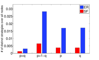
In Figure 5 we report the fraction of different strategies found in a population of ER and SF networks once the dynamical equilibrium is reached. It is clear that in SF networks selection acts stronger than in homogeneous populations since after selection takes place only a few number of strategies remain. We have checked that this is due to the presence of hubs and their ability for replicating their strategies across their surroundings (that usually involve a large fraction of the population). In particular, for the cases of A and B players, we have already shown that a hub can play successfully the UG with a well-mixed population using a broad range of $p$ values; namely, in the thermodynamic limit ($k_{h}\rightarrow\infty$), we have $p_{h}\in[0,1]$ for type A and $p_{h}\in[1/2,1]$ for type B. Any of these values of $p$, when replicated by the well-mixed population in the next generations, increase the payoff difference between hubs and the rest of the individuals. Therefore, the dynamics of the well-mixed population in contact with the hub is finally frozen with the $p$ value dictated by it. From Figure 5 it becomes clear that the same happens for populations of C players. Note also that the fact that the number of different strategies observed during the equilibrium of SF networks is smaller than that in ER networks is not inconsistent with the fact that the distribution $D(p)$ in SF displays long tails since this distribution is constructed averaging over many different equilibria.

Figure 5: Degree of selection, measured as the number of different asymptotic strategies divided by $N$, for ER and SF networks in the three different settings: (A) $p=q$, (B) $p=1-q$ and (C) $p$ and $q$ independent.

4 Social Penalty

In this section, we change the scenario for the selection rule of strategies focusing on the application of the so-called “social penalty” after each round robin of the UG. Let us remark that, with this evolutionary rule, in order to survive a player has to take care not only of its payoff, but also of those of its neighbors, since the poorest player of the network is replaced together with all its neighbors. Therefore, if an individual exploits his neighborhood so that he takes a large stake of the total reward, he would risk to be dropped out of the game as a result of one of his neighbors being that with the lowest payoff in the population of players. Consequently, what drives the evolution of the distribution of $p$ values among the population is the balance between the conflicting interests of earning more (to avoid being the poorest) and earning less (to avoid being stigmatized). This conflict could, in principle, be solved in the case of hubs in SF networks: being the most connected elements, hubs are topological favoured to accumulate a large payoff per round. Therefore a hub can afford large degrees of altruism providing his neighbors with enough payoff to survive and, at the same time, without any risk of being himself the poorest element of the population.

Notice that, at variance with Natural Selection, successful strategies do not replicate but simply survive in the long term. Therefore, as the removed individuals are replaced by new players with randomly chosen strategies the equilibrium is approached slower than in networks driven by Natural Selection. The results presented below correspond to the numerical simularions of the UG dynamics over times up to $t=10^{7}$, and averaged over at least $10^{2}$ different realizations of the networks and initial conditions.

4.1 Networks of type A players ($p=q$)

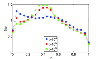
In Figures 6.a and 6.c we show the evolution of the distributions of offers $D(p)$ of type A players at different times. In the case of ER networks (Figure 6.a) the distribution is nearly flat (with slowly decreasing tails at both extremes), pointing out that any strategy can survive in a population of type A players with homogeneous degree. On the other hand, the case of SF networks (Figure 6.c) reveals a more selective population since a large number of individuals offer a quantity around $p\simeq 0.75$. However, although having a well defined maximum, it is evident that nearly all the offers can survive.

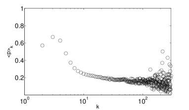
The maximum of SF networks can be explained by looking at the mean offer of players with degree $k$:

$$\langle p\rangle_{k}=\frac{\sum_{\{i|k_{i}=k\}}p_{i}}{NP(k)}\;.$$ (12)

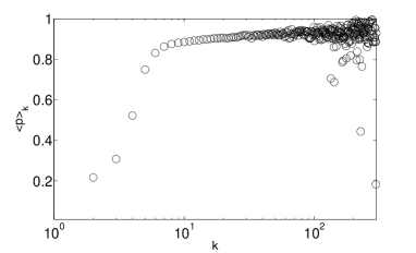
Figure 6.e plots this quantity as a function of the degree $k$. It is evident from the figure that those players with low connectivity (the largest part of the population in SF networks) are the ones playing with the offers around $p\simeq 0.75$. On the other hand, offers from high degree nodes are very low. This latter result points out that hubs are far from being altruistic in the case of a population of type A players. Moreover, in the case of a hub connected to a large number of low degree nodes, the offers from the hub will be automatically rejected since $p_{h}$ is lower than those offered by the leaves. Besides, since most of leaves offer $p>1/2$ to the hub, it takes the largest part of the reward in all its interactions with the leaves. Therefore, hubs exploit their neighboring leaves in a population of type A players, thus contradicting the arguments about the need of generosity from hubs when social penalty is at work.

(a) ER $p=q$

(b) ER $p=1-q$

(c) SF $p=q$

(d) SF $p=1-q$

(e) SF $p=q$

(f) SF $p=1-q$

Figure 6: Distribution of offers $D(p)$ for ER and SF networks in the cases $p=q$ [(a) and (c)] and $p=1-q$ [(b) and (d)] when a Social penalty is used as the update rule. Panels (e) and (f) show the values of $\langle p\rangle_{k}$ as a function of $k$ for the cases $p=q$ and $p=1-q$ in SF networks.

4.2 Networks of type B players ($p=1-q$)

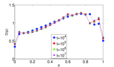
In the case of type B players the stationary distribution of offers $D(p)$ for ER and SF networks are shown in Figures 6.b and 6.d respectively. Interestingly, both distributions show the same average value for the offers $\langle p\rangle\simeq 0.5$. Though of equal average value, the distribution densities are strikingly different for both kind of networks. While for ER networks $D(p)$ is almost flat with slowly decreasing tails at both extremes (such as in the case of type A players), it is bimodal for the SF network. The two local maxima of $D(p)$ in SF networks are placed at $p\simeq 0.3$ and $p\simeq 1$. In principle this result points out the polarization of the population into altruistic and selfish individuals. Therefore, the degree-heterogeneity of SF networks promotes a very different microscopic balance of conflicting aims, as reflected in the bimodal $D(p)$, with respect to the mostly uniform density of strategies observed in near homogeneous networks (ER).

The answer of such bimodal distribution in SF networks can be obtained by looking at Figure 6.f, that shows the dependence of $\langle p\rangle_{k}$ on the degree of the nodes. In this case the mean offer is seen to increase with the degree, in agreement with the expected behavior for high degree nodes in SF networks explained above. Moreover, the hubs of the network display a complete altruistic behavior $p\rightarrow 1$. In this way, since the relation between the offers of two players $p_{i}+p_{j}\geq 1$ must hold in order to conclude a deal, low degree nodes attached to hubs both achieve the former successful combination of offers and maximize its reward by chosing low values of $p$.

It is possible to show that, within the context of a SF network of type B players, hubs can afford full generosity without any risk. Let us define the ”interacting degree” of node $i$, $k_{i}^{int}$, as the number of neighbors of $i$ with whom it interacts successfully (i.e. those satisfying $p_{j}+p_{i}\geq 1$, the interacting neighborhood). If we consider a hub in a SF network, $k_{h}\gg 1$, then under the assumption that $p$ is distributed in its neighborhood following the same distribution as in the whole network, we obtain:

$$k_{h}^{int}=k_{h}\int_{1-p_{h}}^{1}D(p)\;dp=k_{h}\left(1-F(1-p_{h})\right)\;,$$ (13)

where $F$ is the (cumulative) distribution function of $D(p)$. Under the same assumptions, it follows that the payoff received by a hub is

$$\Pi_{h}=k_{h}\left[1-F(1-p_{h})\right]\left[(1-p_{h})+\int_{1-p_{h}}^{1}p\;dF\right]\;,$$ (14)

where the integral is the average of $p$ in the ”interacting” neighborhood of the hub. Provided that this average is larger than $\theta_{b}/k_{h}$, the limit when $p_{h}\rightarrow 1$ is

$$\lim_{p_{h}\rightarrow 1}\Pi_{h}>\theta_{b}\;.$$ (15)

If $\theta_{b}$ is an upper bound of $\min_{i}\Pi_{i}$, then a hub will not have the minimum payoff even if it offers the whole stake and accepts any offer. One can give a simple estimate for the upper bound $\theta_{b}$: For $k_{min}=2$, the less connected nodes offering $0$ and linked to two fully generous neighbors will obtain $4$. That is, we can assume $\theta_{b}\leq 4$, in the argument above. In other words, if the average value of the hubs neighbors $p_{ave}>\theta_{b}/k_{h}$ (which at most is $4/k_{h}$), hubs can give away almost the whole stake. In particular, in the thermodynamic limit where $k_{h}$ diverges, they can offer $p=1$. Therefore, hubs can afford full generosity. Moreover, they minimize the risk of being stigmatized by adopting high values of $p$. In other words, they not only can afford full generosity, but also better they do if they want their neighbors safe.

4.3 Networks of type C players (independent $p$ and $q$)

We analyze now the case when the values of offers $p$ and acceptance thresholds $q$ are independent. After having obtained quite different results in populations of type A and type B players one of our aims here is to unveil whether any of these latter behaviors is also observed when players are free to decide the relation between $p$ and $q$. In Figure 7 we sketch the main results for ER and SF networks.

(a) ER $(p,q)$

(b) SF $(p,q)$

(c) ER $(p,q)$

(d) SF $(p,q)$

(e) $(p,q)$

(f) $(p,q)$

Figure 7: The distributions of offers $D(p)$ [(a) and (b)] and thresholds of acceptance $D(q)$ [(c) and (d)] for ER [(a) and (c)] SF [(b) and (d)] networks when Social Penalty is used as the update rule. Panels (e) and (f) show the values of $\langle p\rangle_{k}$ and $\langle q\rangle_{k}$ as a function of $k$ in SF networks.

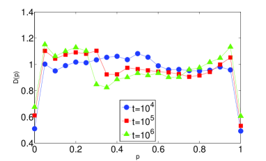
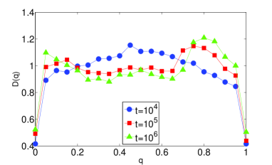
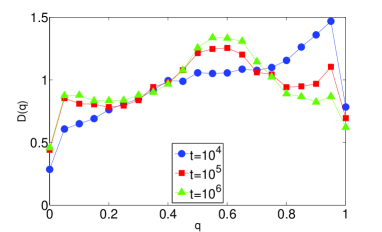
In the case of ER networks we show in Figures 7.a and 7.c the time evolution of the distributions $D(p)$ and $D(q)$ respectively. It is interesting to follow the time evolution of both distributions. While at $t=10^{4}$ roughly all the offers and acceptance thresholds are equally probable, for large enough times the two distributions become bimodal: First, strategies having $p<0.25$ and $q>0.75$ are clearly favored, at the same time, both distributions show a peak at low and high values of $p$ and $q$ respectively. Therefore, the two distributions are slightly polarized towards high and low values of $p$ and $q$.

In SF netwoks the situation is completely different. In Figures 7.b and 7.d we find asymptotic distributions with a well-defined maximum at intermediate values of both $p$ and $q$. In particular the two maxima are placed at $p\simeq 0.4$ and $q\simeq 0.6$ pointing out that population converges to an equilibrium where the mean offer is similar to those values found in experiments whereas the acceptance threshold is larger than typically observed, pointing out an idiosincratic behavior [29]. It is also interesting to report on the time evolution of the two distributions. From the figure it is clear that at moderate times $t=10^{4}$ the population focus on low offers and high acceptance thresholds, a situation in which a few deals can be concluded and thus the global payoff is minimum. At $t=10^{5}$ the low $p$ and high $q$ regions are abandoned and the population tends to concentrate around the maxima of the asymptotic distributions at $t=10^{6}$ and then a large amount of deals can be concluded.

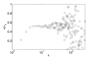
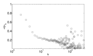
Looking at the distributions of $p$ and $q$ across degree clases, $\langle p\rangle_{k}$ (Figure 7.e) and $\langle q\rangle_{k}$ (Figure 7.f), we see clearly that the population occupying the regions around the maxima of both $D(p)$ and $D(q)$ are those players of low degree. Interestingly, in the case of $\langle p\rangle_{k}$ there is a range, from intermediate to high degrees, where a constant average offer $\langle p\rangle_{k}\simeq 0.5$ is reached. Similarly, in the same range of degrees, the values of the acceptance thresholds stabilize around $\langle q\rangle_{k}\simeq 0.2$. The overall trends of both functions are that $\langle p\rangle_{k}$ grows with the degree (similarly to what is found in SF networks of type B players) whereas $\langle q\rangle_{k}$ decreases with $k$. This indicates that high degree nodes, suported in their topological advantadge, accept the low offers from the leaves and offer a large part of the stake to them, thus favouring their survival.

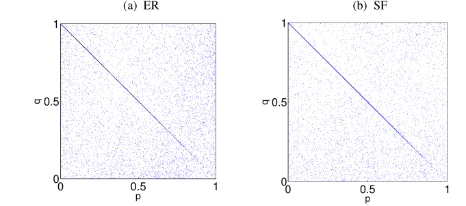
From figures 7.e and 7.f we can conclude a coarse-grained description of the population: Individuals with high (low) values of $p$ display low (high) acceptance thresholds. Although this description is based on average values across degree classes it is clear that the assumption $p=q$ is no longer valid when players are allowd to chose $p$ and $q$ freely. We have checked the true correlation between the individuals values of $p_{i}$ and $q_{i}$ for ER and SF networks. In Figure 8 we show the set values of the pairs $\{(p_{i},q_{i})\}$ obtained in the asymptotic regime. Surprisingly, the accumulation of points along the curve $p=1-q$ points out that social penalty promote the behavior as type B players of large part of the population in both topologies. This result validates the assumption made above about the two strategic groups in SF networks. Additionally, the observed trend $p=1-q$ nicely explains the composition of the two peaks observed in the distributions $D(p)$ and $D(q)$ in ER networks: the maximum corresponding to large (low) offers is formed by the same individuals that form the maximum at low (large) acceptance thresholds.

Figure 8: Scatter plot of the individual strategies $(p_{i},q_{i})$ in the asyntotic regime for ER (a) and SF (b) networks. For the both the ER and SF case we plot the population of $10^{4}$ randomly chosen realizations, In both topologies the most frequent combination that emerges is $p_{i}=1-q_{i}$, resembling the case of players of type B.

5 Discussion and Conclusions

We have studied the Ultimatum Game when the individulas play among them according to a network of interactions. In the networks considered in this study individuals can have an homogenous number of neighbors (Erdös-Rènyi graphs) or, on the contrary, present a high degree of heterogeneity in the number of contacts (Scale-free networks). From this perspective, we analyze how the existence of different connectivity classes in scale-free networks affects the behavior of the system. The Ultimatum Game dynamics has been studied under three different frameworks: (i) role distinguishing, or empathetic, agents (players offer the same quantity they want to be offered), (ii) role ignoring, or pragmatic, agents (players want to obtain the same amount both as responders and proposers) and (iii) agents with independent values for offers and acceptance thresholds. Besides, we have explored two different mechanisms for implementing the selection rule at each generation, namely: (i) Natural Selection, according to which players replicate the fittest agents, and (ii) Social Penalty, according to which, at each generation, the poorest agent is removed together with his neighbors.

Within the context of Natural selection we have observed that the results derived from well-mixed arguments for the case of role distinguishing and role ignoring agents agree well with those obtained in degree homogeneous populations, where the distributions of offers are quite focused around $50\%$. Instead, in the case of heterogeneous networks, the presence of highly connected nodes change quantitatively (not qualitatively) the distribution making it broader, since hubs can afford to make nearly all possible offers. When agents are allowed to choose their offers and thresholds of acceptance independently, offers tend to decrease in both Erdös-Rènyi and scale-free graphs to the $40\%$. Surprisingly, thresholds of acceptance are remarkably low, although they are still far from the rational economic behavior and almost any offer above the $30\%$ of the stake is accepted. Therefore altruistic punishment, understood as the rejection of low offers, arises in the context of Natural selection regardless of the underlying topology.

(a) Natural Selection $(p,q)$

(b) Natural Selection $(p,q)$

(c) Social Penalty $(p,q)$

(d) Social Penalty $(p,q)$

Figure 9: The distributions of offers $D(p)$ [(a) and (c)] and thresholds of acceptance $D(q)$ [(b) and (d)] for natural Selection [(a) and (b)] and Social Penalty [(c) and (d)] settings on SF networks. The networks are generated using the model in [39] and $p$ and $q$ are independent.

Interestingly, the replication of fittest strategies provokes that the selection of strategies in the asymptotic regime is remarkably high, especially in the case of scale-free networks. This selection is explained in terms of the existence of hubs and their ability to obtain a large reward with a broad range of strategies and thus to dictate the final behavior of the entire population.

When Social punishment is implemented the dynamical behavior of the system changes radically. Within this selection rule agents have to take care not only about their own benefit but also about the fitness of their neighbors. Within this context, we have found two drastically different behaviors between empathetic and pragmatic agents. In particular, for scale-free networks, low degree nodes and high degree nodes display opposite behaviors in the two settings. On one hand, in a population of role distinguishing agents, leaves are those proposing a large portion of the stake (above $50\%$) whereas hubs show low offers (below $20\%$). On the other hand, for role ignoring agents the situation is the opposite, since large offers (nearly the $100\%$) come from hubs while leaves display selfish behavior. It is therefore in this latter setting where true altruistic behavior is observed. Note that altruism arises in a self-organized manner with selection acting locally: highly connected agents optimize their chances to survive by increasing their generosity, without risking to be the poorest in town.

Probably the most interesting result is obtained when, in the framework of Social punishment, players can adapt their offers and acceptance thresholds independently. Surprisingly, the dynamical equilibria of both homogeneous and heterogeneous networks resemble to a large extent that of role ignoring agents. In particular we have shown that, in SF network, the large degree nodes, although not displaying full altruism, offer a large reward (more than $50\%$) to their neighbors and accept low offers (below $20\%$). On the other hand, the opposite behavior is found in lowly connected players. We have further confirmed that, in the long run, players adapt their strategies and converge to the setting of role ignoring agents, the framework where full altruistic behavior is observed. Let us remark that the abundance of highly generous individuals observed when Social Penalty is at work does not arise due to reputation [36], nor costly individuals’ punishment [30], but from a purely scale-free effect combined with a social enforcement of altruism.

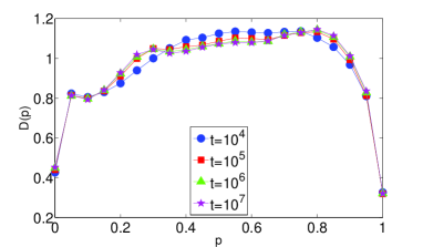
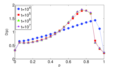
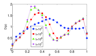
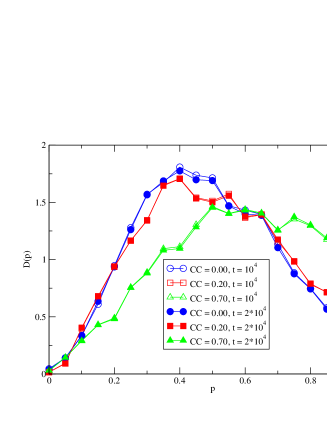
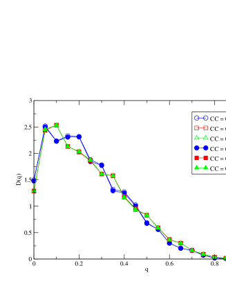
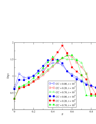
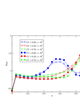
Finally, we point out that a full and satisfactory understanding of the models exposed here may likely demand to study the dependence on other important topological features (such as the clustering coefficient, degree-degree correlations, etc) or to incorporate the competition between different kinds of individuals (role-ignoring and role-distinguishing) into the model formulation. In particular, we have explored how our results change when the underlying SF networks have a non-vanishing clustering coefficient when $p$ and $q$ are independent (type C players). This is not an easy issue, as one should first construct networks with a tunable clustering coefficient while keeping the rest of topological properties unaltered. The model proposed in [39] can be used to such an study as it generates scale-free networks with varying clustering properties but leaving the rest of topological features roughly the same. Our results indicate that no general conclusion can be reached as the effects of the clustering depend on several factors, of both topological and dynamical nature. As shown in Fig. 9, in the case of natural selection, the distribution $D(q)$ does not change when the clustering coefficient of the networks is increased from 0 to 0.7, while $D(p)$ changes if the clustering coefficient exceeds 0.2 in such a way that the average offer increases. On the contrary, for the social penalty setting, $D(p)$ remains roughly unaltered whatever the clustering of the network is, whereas $D(q)$ deviates from its behavior for non-clustered networks as soon as the clustering coefficient is increased leading to a distribution with a peak at very high acceptance thresholds. All these are aspects to further explore in future works.

References

- [1] S. J. Gould, The Structure of Evolutionary Theory, Harvard University Press, Cambridge, 2002.
- [2] G. Vogel, Science 303, 1128 (2004).
- [3] W. D. Hamilton, J. Theor. Biol. 7, 1 (1964).
- [4] M. A. Nowak and K. Sigmund, Nature 393, 573 (1998).
- [5] M. Milinski, D. Semmann, and H. J. Krambeck, Nature 415, 424 (2002).
- [6] M. A. Nowak, Evolutionary Dynamics. Exploring the Equations of Life. (Harvard University Press, Harvard, 2006).
- [7] E. Fehr and S. Gächter, Nature 415, 137 (2002).
- [8] H. Gintis, S. Bowles, R. Boyd, and E. Fehr, Evol. Hum. Behav. 24, 153 (2003).
- [9] E. Fehr and U. Fischbacher, Nature 425, 785 (2003).
- [10] J. H. Fowler, Proc. Nat. Ac. Sci 102, 7047 (2005).
- [11] A. Sánchez and J. A. Cuesta, J. Theor. Biol. 235, 233 (2005).
- [12] M. E. J. Newman, SIAM Rev. 45, 167 (2003).
- [13] S. Boccaletti, V. Latora, Y. Moreno, M. Chavez, and D. U. Hwang, Phys. Rep. 424, 175 (2006).
- [14] R. Pastor-Satorras and A. Vespignani, Phys. Rev. Lett. 86, 3200 (2001).
- [15] Y. Moreno, R. Pastor-Satorras and A. Vespignani, Eur. Phys. J. B 26, 521 (2002).
- [16] Y. Moreno, M. Nekovee and A. F. Pacheco, Phys. Rev. E 69, 066130 (2004).
- [17] A. Arenas, A. Díaz-Guilera, J. Kurths, Y. Moreno and C. Zhou, Phys. Rep. 469, 93 (2008).
- [18] G. Szabó and G. Fáth, Phys. Rep. 446, 97 (2007).
- [19] F. C. Santos, and J. M Pacheco, Phys. Rev. Lett. 95, 098104 (2005).
- [20] F. C. Santos, J. M. Pacheco and T. Lenaerts, Proc. Nat. Acad. Sci. USA 103, 3490 (2006).
- [21] J. Gómez-Gardeñes, M. Campillo, L. M. Floría and Y. Moreno, Phys. Rev. Lett. 98, 108103 (2007).
- [22] J. Poncela, J. Gómez-Gardeñes, L. M. Floría and Y. Moreno, New Jour. Phys. 9, 184 (2007).
- [23] J. Gómez-Gardeñes, J. Poncela, L. M. Floría and Y. Moreno, J. Theor. Biol. 253, 296 (2008).
- [24] V. Hatzopoulos and H. J. Jensen, Phys. Rev E. 78, 011904 (2008).
- [25] F. C. Santos, M. D. Santos and J. M. Pacheco, Nature 454 213 (2008).
- [26] W. Güth, R. Schmittberger and B. Schwarze, J. Econ. Behavior and Organization 3, 367 (1982).
- [27] K. M. Page, M. A. Nowak, and K. Sigmund, Proc. R. Soc. Lond. B 267 2172 (2000).
- [28] C. F. Camerer, Behavioral Game Theory. (Russell Sage Foundation, Princeton University Press, Princeton, 2003).
- [29] J. Henrich, R. Boyd, S. Bowles, C. Camerer, E. Fehr, and H. Gintis (eds.), Foundations of Human Sociality: Economic Experiments and Ethnographic Evidence from Fifteen Small-Scale Societies, (Oxford University Press, Oxford, 2004).
- [30] A. Dreber, D. G. Rand, D. Fudenberg and M. A. Nowak, Nature 452, 348 (2008).
- [31] P. Bak and K. Sneppen, Phys. Rev. Lett. 71, 4083 (1993).
- [32] Y. Moreno and A. Vázquez, Europhys. Lett. 57, 765 (2002).
- [33] D. Eriksson and H. J. Jensen, J. Stat. Mech.: Theor. Exp. P09001 (2004).
- [34] J. Gómez-Gardeñes and Y. Moreno, Phys. Rev. E 73, 056124 (2006).
- [35] K. M. Page, and M. A. Nowak, Bull. Math.Biol. 64, 1101 (2002).
- [36] M. A. Nowak, K. M. Page, and K. Sigmund, Science 289, 1773 (2000).
- [37] D. Helbing, Physica A 181, 29 (1992).
- [38] D. Helbing, in Economic evolution and demographic change G. Hagg, U. Mueller, and K. G. Troitzsch (eds.), (Springer-Verlag, Berlin, 1992).
- [39] P. Holme and B.J. Kim, Phys. Rev. E 65, 026107 (2002).