Collisional and Thermal Emission Models of Debris Disks:
Towards Planetesimal Population Properties

Abstract

Debris disks around main-sequence stars are believed to derive from planetesimal populations that have accreted at early epochs and survived possible planet formation processes. While debris disks must contain solids in a broad range of sizes — from big planetesimals down to tiny dust grains — debris disk observations are only sensitive to the dust end of the size distribution. Collisional models of debris disks are needed to “climb up” the ladder of the collisional cascade, from dust towards parent bodies, representing the main mass reservoir of the disks. We have used our collisional code to generate five disks around a sun-like star, assuming planetesimal belts at 3, 10, 30, 100, and $200\,\mbox{AU}$ with 10 times the Edgeworth-Kuiper-belt mass density, and to evolve them for 10 Gyr. Along with an appropriate scaling rule, this effectively yields a three-parametric set of reference disks (initial mass, location of planetesimal belt, age). For all the disks, we have generated spectral energy distributions (SEDs), assuming homogeneous spherical astrosilicate dust grains. A comparison between generated and actually observed SEDs yields estimates of planetesimal properties (location, total mass etc.). As a test and a first application of this approach, we have selected five disks around sun-like stars with well-known SEDs. In four cases, we have reproduced the data with a linear combination of two disks from the grid (an “asteroid belt” at $3\,\mbox{AU}$ and an outer “Kuiper belt”); in one case a single, outer component was sufficient. The outer components are compatible with “large Kuiper belts” of 0.2–50 earth masses (in the bodies up to $100\,\mbox{km}$ in size) with radii of $100$–$200\,\mbox{AU}$.

1. Introduction

Since the IRAS discovery of the excess infrared emission around Vega by Aumann et al. (1984), infrared surveys with IRAS, ISO, Spitzer, and other space-based and ground-based telescopes have shown the Vega phenomenon to be common for main-sequence stars (e.g. Meyer et al., 2004; Beichman et al., 2005; Najita & Williams, 2005; Rieke et al., 2005; Bryden et al., 2006; Siegler et al., 2007; Su et al., 2006; Trilling et al., 2007; Hillenbrand et al., 2008; Trilling et al., 2008). The observed excesses are attributed to circumstellar disks of second-generation dust, sustained by numerous planetesimals in orbit around the stars. Jostling collisions between planetesimals grind them all the way down to smallest dust grains which are then blown away by stellar radiation. While the bulk of such a debris disk’s mass is hidden in invisible parent bodies, the observed luminosity is dominated by small particles at dust sizes. Hence the studies of dust emission have a potential to shed light onto the properties of parent planetesimal populations as well as planets that may shape them and, ultimately, onto the evolutionary history of circumstellar planetary systems.

However, there is no direct way to infer the properties of invisible planetesimal populations from the observed dust emission. Dust and planetesimals can only be linked through models. First, dynamical models can be used to predict, for a given planetesimal family (mass, location, age, etc.), the distribution of dust. Such models have become available in recent years (e.g. Thébault et al., 2003; Krivov et al., 2006; Thébault & Augereau, 2007; Wyatt et al., 2007; Löhne et al., 2008). After that, standard thermal emission models will describe the resulting dust emission. Comparison of that emission to the one actually observed would then reveal the probable properties of underlying, dust-producing planetesimal families.

In this paper, we follow this approach and generate a set of hypothetical debris disks around G2 dwarfs with different ages (10 Myr – 10 Gyr), assuming debris dust to stem from planetesimal belts with different initial masses at different distances from the central star. For every set of these parameters, we simulate steady-state dust distributions with our collisional code (Krivov et al., 2005, 2006; Löhne et al., 2008). This is different from a traditional, “empirical” approach, in which dust distributions are postulated, usually in form of power laws, parameterized by ranges and exponents that play a role of fitting parameters (e.g. Wolf & Hillenbrand, 2003). Interestingly, replacing formal dust distributions with those coming out of dynamical modeling does not increase the number of fitting parameters. Just the opposite: the number of parameters reduces and those parameters that we keep free all have clear astrophysical meaning. The most important are location of a parent planetesimal belt and its current mass (Wyatt et al., 2007).

Having produced a set of model debris disks, we compute thermal emission fluxes in a wide range of wavelengths from mid-infrared to millimeter. In so doing, we completely abandon simple blackbody or modified blackbody calculations and solve a thermal balance equation instead. At this stage, we assume compact spherical grains composed of astronomical silicate (Laor & Draine, 1993) and employ standard Mie calculations to compute dust opacities. Although this is still a noticeable simplification, it represents a natural step towards considering realistic materials and using more involved methods of light scattering theory that we leave for subsequent papers.

As a test and a first application of the results, we re-interprete available observational data on a selection of disks around sun-like stars with well known spectral energy distributions (SEDs).

This paper is organized as follows. Section 2 describes the dynamical and thermal emission models. In section 3, a set of reference disks is introduced and the model parameters are specified. Section 4 presents the modeling results for this set of disks: size and spatial distribution of dust, dust temperatures, and the generated SEDs. Application to selected observed disks is made in section 5. Section 6 summarizes the paper.

2. Model

2.1. Dynamical model

To simulate the dust production by the planetesimal belt and the dynamical evolution of a disk, we use our collisional code (ACE, Analysis of Collisional Evolution). The code numerically solves the Boltzmann-Smoluchowski kinetic equation to evolve a disk of solids in a broad range of sizes (from smallest dust grains to planetesimals), orbiting a primary in nearly Keplerian orbits (gravity + direct radiation pressure + drag forces) and experiencing disruptive and erosive (cratering) collisions. Collision outcomes are simulated with available material- and size-dependent scaling laws for fragmentation and dispersal in both strength and gravity regime. The current version implements a 3-dimensional kinetic model, with masses, semimajor axes, and eccentricities as phase space variables. This approach automatically enables a study of the simultaneous evolution of mass, spatial, and velocity distribution of particles. The code is fast enough to easily follow the evolution of a debris disk over Gyr timescales. A detailed description of our approach, its numerical implementation, and astrophysical applications can be found in our previous papers (Krivov et al., 2000, 2005, 2006; Löhne et al., 2008).

2.2. Thermal emission model

For spherical dust grains with radius $s$ and temperature $T_{\mathrm{g}}$ we can calculate their distance $r$ to the star under the assumption of thermal equilibrium as

$$r=\frac{R_{*}}{2}\sqrt{\frac{\int_{0}^{\infty}\,\mbox{d}\lambda\;Q_{\lambda}^{\mathrm{abs}}(s)F_{\lambda,*}(T_{*})}{\int_{0}^{\infty}\,\mbox{d}\lambda\;Q_{\lambda}^{\mathrm{abs}}(s)B_{\lambda}(T_{\mathrm{g}})}}.$$ (1)

Here, $R_{*}$ denotes the radius and $F_{\lambda,*}(T_{*})$ the flux of the star with an effective temperature $T_{*}$ and $B_{\lambda}(T_{\mathrm{g}})$ the Planck function. The absorption efficiency $Q_{\lambda}^{\mathrm{abs}}(s)$ is a function of wavelength $\lambda$ and particle size.

We now consider a rotationally symmetric dust disk at a distance $D$ from the observer. Denote by $N(r,s)$ the surface number density of grains with radius $s$ at a distance $r$ from the star, so that $N(r,s)ds$ is the number of grains with radii $[s,s+ds]$ in a narrow annulus of radius $r$, divided by the surface area of that annulus. Then the specific flux emitted from the entire disk at a given wavelength can be calculated as

$$F_{\lambda,\mathrm{disk}}^{\mathrm{tot}} = \int\,\mbox{d}r\int\,\mbox{d}s\;F_{\lambda,\mathrm{disk}}(r,s)$$ (3)

$$= \frac{2\pi^{2}}{D^{2}}\int\,\mbox{d}T_{g}\,r(T_{g})\,\frac{\,\mbox{d}r(T_{g})}{\,\mbox{d}T_{g}}\int\,\mbox{d}s\;s^{2}\;\times$$

$$\times\;N(r,s)\,Q_{\lambda}^{abs}(s)\,B_{\lambda}(T_{g}).$$

3. Reference disks

3.1. Central star

The parameters of the central star (mass and photospheric spectrum) affect both the dynamics of solids (by setting the scale of orbital velocities and determining the radiation pressure strength) and their thermal emission (by setting the dust grain temperatures). We take the Sun (a G2V dwarf with a solar metallicity) as a central star and calculate its photospheric spectrum with the NextGen grid of models (Hauschildt et al., 1999).

3.2. Forces

In the dynamical model, we include central star’s gravity and direct radiation pressure. We switch off the drag forces (both the Poynting-Robertson and stellar wind drag), which are of little importance for the optical depths in the range from $\sim 10^{-5}$ to $\sim 10^{-3}$) considered here (Artymowicz, 1997; Krivov et al., 2000; Wyatt, 2005).

3.3. Collisions

The radii of solids in every modeled disk cover the interval from $0.1\,\mu\hbox{m}$ to $100\,\mbox{km}$. The upper limit of $100\,\mbox{km}$ is justified by the fact that planetesimal accretion models predict larger objects to have a steeper size distribution and thus to contribute less to the mass budget of a debris disk (e.g. Kenyon & Luu, 1999b). To describe the collisional outcomes, we make the same assumptions as in Löhne et al. (2008). This applies, in particular, to the critical energy for disruption and dispersal, $Q_{D}^{*}(s)$, as well as to the size distribution of fragments of an individual collision. However, in contrast to Löhne et al. (2008) where only catastrophic collisions were taken into account, we include here cratering collisions as well. This is necessary, as cratering collisions alter the size distribution of dust in the disk markedly, which shows up in the SEDs (Thébault et al., 2003; Thébault & Augereau, 2007). The actual model of cratering collisions used here is close to that by Thébault & Augereau (2007). An essential difference is our assumption of a single power law for the size distribution of the fragments of an individual collision instead of the broken power law proposed originally in Thébault et al. (2003). However, this difference has little effect on the resulting size distribution in collisional equilibrium.

3.4. Optical properties of dust

An important issue is a choice of grain composition and morphology. These affect both the dynamical model (through radiation pressure efficiency as well as bulk density) and thermal emission model (through absorption efficiency). Here we assume compact spherical grains composed of astronomical silicate (a.k.a. astrosilicate or astrosil, Laor & Draine, 1993), similar to the MgFeSiO₄ olivine, with density of $3.3\,\mbox{g}\,\mbox{cm}^{-3}$. Taking optical constants from Laor & Draine (1993), we calculated radiation pressure efficiency $Q_{pr}$ and absorption efficiency $Q_{abs}$ with a standard Mie routine (Bohren & Huffman, 1983).

To characterize the radiation pressure strength, it is customary to use the radiation pressure to gravity ratio $\beta$ (Burns et al., 1979), which is independent of distance from the star and, for a given star, only depends on $Q_{pr}$ and particle size. If grains that are small enough to respond to radiation pressure derive from collisions of larger objects in nearly circular orbits, they will get in orbits with eccentricities $e\sim\beta/(1-\beta)$. This implies that grains with $\beta<0.5$ remain orbiting the star, whereas those with $\beta>0.5$ leave the system in hyperbolic orbits. The $\beta$ ratio for compact astrosil grains, computed from $Q_{pr}$, is shown in Fig. 1. The blowout limit, $\beta=0.5$, corresponds to the grain radius of $s=0.4\,\mu\hbox{m}$. Note that the tiniest astrosil grains ($\lesssim 0.1\,\mu\hbox{m}$) would have $\beta<0.5$ again and thus could orbit the star in bound orbits. However, the dynamics of these small motes would be subject to a variety of effects (e.g. the Lorentz force) not included in our model, and their lifetimes may be shortened by erosion processes (e.g. stellar wind sputtering). Altogether, we expect them to make little contribution to the thermal emission in the mid-IR to sub-mm. By setting the minimum radius of grains to $0.1\,\mu\hbox{m}$, we therefore do not take into account these grains here.

Figure 1.— Radiation pressure to gravity ratio $\beta$ for astrosilicate grains as a function of their size. Horizontal lines at $\beta=0.5$ and $\beta=1.0$ show, which particles typically move in bound elliptic orbits, in hyperbolas, as well as in anomalous hyperbolas (open outward from the star).

The spectral dependence of the absorption efficiency $Q_{abs}$ of different-sized astrosil spheres is depicted in Fig. 2.

Figure 2.— Top: absorption efficiency of astrosilicate compact spherical grains as a function of wavelength for different grain sizes. Bottom: the spectrum of a G2 V star and the Planck curves for 150 and 20 K (in arbitrary vertical scale) to indicate the spectral ranges most important for absorption and emission.

3.5. Parent planetesimal belts

To have a representative set of “reference” debris disks around sun-like stars, we consider possible planetesimal rings centered at the semimajor axes of $a=3$, $10$, $30$, $100$, and $200\,\mbox{AU}$ from the primary. All five rings are assumed to have the same relative width initially (again, in terms of semimajor axis) of $\Delta a/a=0.2$ ($\pm 0.1$) and share the same semi-opening angle (the same as the maximum orbital inclination of the objects) of $\varepsilon=0.1$ rad. The orbital eccentricities of planetesimals are then distributed uniformly between 0.0 and 0.2, in accordance with the standard equipartition condition. The initial (differential) mass distribution of all solids is given by a power law with the index $1.87$, a value that accounts for the modification of the classical Dohnanyi’s (1969) $1.833$ through the size dependence of material strength (see, e.g., Durda & Dermott, 1997).

Table 1Description of reference disks

Disk	Belt	Initial	$a$ range	$r$ range
identifier	location [AU]	disk mass [$M_{\oplus}$]	[AU]	[AU]
10EKBD @ 003AU	3	0.001	0.3 – 30	0.5 – 20
10EKBD @ 010AU	10	0.03	1 – 100	2 – 50
10EKBD @ 030AU	30	1	3 – 300	5 – 200
10EKBD @ 100AU	100	30	10 – 1000	20 – 500
10EKBD @ 200AU	200	200	20 – 2000	30 – 1000

The initial disk mass is taken to be $1M_{\oplus}$ (earth mass) for a $30\,\mbox{AU}$ ring, roughly corresponding to ten (or slightly more) times the Edgeworth-Kuiper belt (EKB) mass (e.g. Gladman et al., 2001; Hahn & Malhotra, 2005). For other parent ring locations, the initial mass is taken in such a way as to provide approximately the same spatial density of material. Since the circumference of a ring $2\pi a$, its absolute width $\Delta a$, and vertical thickness $2a\varepsilon$ are all proportional to $a$, the condition of a constant density requires the mass scaling $\propto a^{3}$. This corresponds to the initial mass ranging from $\approx 0.001M_{\oplus}$ in the $3\,\mbox{AU}$ case to $\approx 200M_{\oplus}$ in the $200\,\mbox{AU}$ case. With these values, all reference disks have about ten times the EKB density (10 EKBD).

That all the belts share the same volume density of material is purely a matter of convention. Instead, we could choose them to have the same surface density or the same total mass. Given the scaling rules, as discussed in the text and Appendix A, none of these choices would have strong advantages or disadvantages.

All five reference disks are listed in Table 1. We evolved them with the collisional code, ACE, and stored all results between the ages of 10 Myr and 10 Gyr at reasonable time steps. In what follows, we use self-explanatory identifiers like 10EKBD @ 10AU @ 300Myr to refer to a particular disk of a particular age.

Importantly, the same runs of the collisional code automatically provide the results for disks of any other initial density (or mass). This is possible due to the mass-time scaling of Löhne et al. (2008), which can be formulated as follows. Denote by $M(M_{0},t)$ the mass that a disk with initial mass $M_{0}$ has at time $t$. Then, the mass of another disk with $x$ times larger initial mass at time instant $t/x$ is simply

$$M(xM_{0},t/x)=xM(M_{0},t),$$ (4)

For instance, the mass of the 1EKBD @ 10AU @ 10Gyr disk is one-tenth of the 10EKBD @ 10AU @ 1Gyr disk mass. Note that the same scaling applies to any other quantity directly proportional to the amount of disk material. In other words, $M$ may equally stand for the mass of dust, its total cross section, thermal radiation flux, etc. See Appendix A for additional explanations.

4. Results

4.1. Size and spatial distributions of dust

As noted above, the collisional code ACE uses masses and orbital elements of disk particles as phase space variables. At any time instant, their phase space distribution is transformed to usual mass/size and spatial distributions. It is important to understand that mass/size distributions and spatial distributions cannot, generally, be decoupled from each other. Grains of different sizes have different radial distributions and conversely, the size distribution of material is different at different distances from the star.

A typical size distribution of solids is shown in Fig. 3 for one of the disks, namely for 10EKBD @ 30AU @ 100Myr. Different lines correspond to different distances from the primary. As expected, the size distribution is the broadest within the parent ring of planetesimals. Farther out, it only contains grains which are small enough to develop orbits with sufficiently large apocentric distances due to radiation pressure.

Figure 3.— Size distribution in the 10EKBD @ 30AU @ 100Myr disk at three different distances from the star.

The spatial distribution of material in the same disk is shown in Fig. 4. Here, different lines refer to different particle sizes. The ring of the biggest particles shown ($100\,\mu\hbox{m}$), for which radiation pressure is negligible, nearly coincides with the initial ring of planetesimals (semimajor axes: from $27$ to $33\,\mbox{AU}$, eccentricities: from 0.0 to 0.2, hence radial distances from $22$ to $40\,\mbox{AU}$). The larger the particles, the more confined their rings. The rings are more extended outward with respect to the parent planetesimal ring than inward.

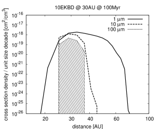
Figure 4.— Spatial distribution of grains with three characteristic radii for the 10EKBD @ 30AU @ 100Myr disk. The ring of the biggest particles shown ($100\,\mu\hbox{m}$, hatched) is the narrowest. Its radial extension is nearly the same as that of the initial planetesimal ring; vertical “walls” are artifacts due to a discrete distance binning.

Radial profiles of the normal geometrical optical depth for three reference disks (planetesimal rings at $10$, $30$, and $100\,\mbox{AU}$) are depicted in Fig. 5. Initially, the peak optical depth of the disks is proportional to the distance of the parent ring, making the $100\,\mbox{AU}$ disk ten times optically thicker than the $10\,\mbox{AU}$ one. The subsequent collisional evolution of the disks depends on their initial mass and distance from the star, as explained in detail in Löhne et al. (2008) and Appendix A. Once a collisional steady state is reached (which is the case after 10 Myr for all three disks), the optical depth decays with time approximately as $t^{\xi}$, where $\xi\approx{-0.3\ldots-0.4}$, i.e. roughly by one order of magnitude from 10 Myr to 10 Gyr. In a steady-state regime, the optical depth is proportional to $r^{1+1.3\xi}\sim r^{1.5}$. This explains why, at any age between 10 Myr and 10 Gyr, the $100\,\mbox{AU}$ ring is $\approx 30$ times optically thicker than the $10\,\mbox{AU}$ one.

Figure 5.— Radial profiles of the normal geometrical optical depth for three out of five basic runs (10EKBD @ 10AU, solid lines; 10EKBD @ 30AU, dashed; 10EKBD @ 100AU, dotted) at different ages. The thinner the line, the older the disk, as marked in the legend. The dashed-dotted lines are initial optical depths, artificially enhanced by a factor of ten for a better visibility.

4.2. Dust temperatures

Figure 6 shows the dust temperatures as a function of two variables: grain distances from the star and their radii. In a parallel scale on the right, we show typical size distributions (cf. Fig. 3). Similarly, under the temperature plot, typical radial profiles of the disk are drawn (cf. Fig. 4). This enables a direct “read-out” of the typical temperature in one or another disk. We find, for example, $130\,\mbox{K}$ at $10\,\mbox{AU}$, $90\,\mbox{K}$ at $30\,\mbox{AU}$, and $50\,\mbox{K}$ at $100\,\mbox{AU}$.

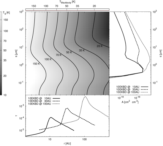
Figure 6.— The left upper plot shows the equilibrium temperature of dust particles as a function of their distance from the star (horizontal axis) and size (vertical axis). Contours are isotherms. The blackbody dust temperatures are given along the upper edge of the plot for comparison. In the right-hand plot the size distribution at the “central” distance of the systems ($10\,\mbox{AU}$, solid; $30\,\mbox{AU}$, dashed; and $100\,\mbox{AU}$, dotted) at 100 Myr is given. The lowest left plot gives the normal optical depth for the same three disks as a function of distance to the star. An intersection of a horizontal straight line going through the maximum of the size distribution in a disk (right) with a vertical line through the peak of its radial profile (bottom) provides the typical dust temperature in that disk.

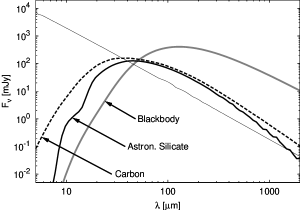
Figure 7.— The emission from one and the same, 1EKBD @ 30AU @ 100Myr, disk, calculated under different assumptions about absorbing and emitting properties of dust grains: blackbody, astrosil (our nominal case), and amorphous carbon particles. Thin solid line: photosphere of a G2V star.

Figure 8.— Spectral energy distributions of disks stemming from planetesimal rings with different masses at different locations and at different time steps. To obtain the absolute values of fluxes, a distance of 10 pc was assumed. Left: reference disks (10EKBD), right: less massive disks (1EKBD). The results for the latter have been obtained with the aid of Eq. (4). From top to bottom: the SEDs of the simulated planetesimal rings at 10, 30 and $100\,\mbox{AU}$. In each panel, lines of decreasing thickness correspond to the ages of 10 Myr, 100 Myr, 1 Gyr, and 10 Gyr. Note that the evolution of the 1EKBD @ 100AU disk at the beginning is very slow, so that the SEDs at 10 and 100 Myr are indistinguishable. Vertical lines indicate centers of observational bands of several instruments (in $\,\mu\hbox{m}$): Spitzer MIPS (24, 70, 160), Herschel PACS (100, 160), Sofia HAWC (200), CSO Sharc (350), JCMT SCUBA/SCUBA 2 (450, 850), MPIfR IRAM (1300). A thin line from top left to bottom right is the stellar photosphere.

Figure 9.— Contribution of individual grain size decades (shown with different linestyles in the left panel) and individual radial annuli of the disks (different linestyles, right) to the SED. As the grain blowout radius is $\approx 0.4\,\mu\hbox{m}$, see Fig. 1, in the left panels we split the lowest size decade into blowout grains with $s\in[0.1\,\mu\hbox{m},0.4\,\mu\hbox{m}]$ and bound ones with $s\in[0.4\,\mu\hbox{m},1.0\,\mu\hbox{m}]$. Panels from top to bottom correspond to planetesimal rings at 10, 30 and $100\,\mbox{AU}$. The initial density of all disks is 10EKBD and their age is 1 Gyr.

These values are noticeably higher than the blackbody values of $88\,\mbox{K}$, $51\,\mbox{K}$, and $28\,\mbox{K}$, respectively. The reason for these big deviations and for the S-shaped isotherms in Fig. 6 is the astronomical silicate’s spectroscopic properties with relatively high absorption at visible wavelengths and steeply decreasing absorption coefficient at longer wavelengths (see Fig. 2). The cross-section dominating astrosil grains are in a size range where the absorption efficiency for visible and near-infrared wavelengths (around $1\,\mu\hbox{m}$) has already reached the blackbody value while emission is still rather inefficient. With the enhancement of the emission efficiencies relative to the “saturated” absorption, temperatures drop drastically for somewhat larger grains. The larger the distance from the star (yielding lower average temperature and lower emission efficiency), the wider the size range over which the temperature decreases, and the stronger the temperature difference between small and large grains. This explains why the S-shape of the isotherms gets more pronounced from the left to the right in Fig. 6.

Further, we note that Mie resonances can increase the absorption/emission efficiencies even beyond unity for wavelengths somewhat longer than the grain size (see $1\,\mu\hbox{m}$, $10\,\mu\hbox{m}$, and $100\,\mu\hbox{m}$ curves in Fig. 2). This explains the temperature maximum for grains of about $0.3\,\mu\hbox{m}$ radius (“resonance” with the stellar radiation maximum) and the minimum with temperatures even below the blackbody values for 10 to $50\,\mu\hbox{m}$ grain radius (“resonance” with the blackbody emission peak).

4.3. Spectral energy distributions

We start with a single, “typical” SED for one of the disks. Such an SED for the 1EKBD @ 30AU @ 100Myr disk is shown in Fig. 7 with a thick solid line. It peaks at about $50\,\mu\hbox{m}$, which is consistent with the dust temperatures (Fig. 6). The hump at $\approx 10\,\mu\hbox{m}$ is due to a classical silicate feature, as discussed below.

For comparison, we have overplotted the SEDs calculated for the same disk, but under different assumptions about the absorbing and emitting properties of grains: in a black-body approximation (grey line) and for amorphous carbon (dashed line). Note that the difference applies only to the calculation of thermal emission. In other words, the dynamical modeling was still done by assuming the radiation pressure of astrosil and not of perfectly absorbing or carbon particles, but we assumed the grains to absorb and emit like a blackbody or carbon when calculating the thermal emission. There is a striking difference between the curves, especially the blackbody SED deviates from the others dramatically. The blackbody assumption leads to a strong increase of the total flux as well as to a shift of the maximum in the SED from 50 to $130\,\mu\hbox{m}$! In addition the excess drops towards longer wavelengths much slower than in the case of the astronomical silicate. In fact, it will never intersect the stellar photospheric flux.

We now proceed with a set of SEDs for our grid of reference disks. Some of them are shown in Fig. 8. The main features of these plots reveal no surprises. The absolute level of excess emission is higher for more massive disks, as well as for distant ones (which is just the consequence of the assumed “same-density” scaling, as described in Sect. 3.5, see also Fig. 5). The amount of dust emission is roughly comparable with the photospheric emission for the mid-aged 1EKBD @ 30AU disk. This is consistent with the known fact that a several Gyr-old EKB counterpart would only slightly enhance the photospheric emission even at the “best” wavelengths. The position of the maximum emission ranges from $\approx 30\,\mu\hbox{m}$ for the $10\,\mbox{AU}$ disk to $\approx 70\,\mu\hbox{m}$ for the $100\,\mbox{AU}$ disk. Note that blackbody calculation would predict the emission to peak at longer wavelengths; beyond $100\,\mu\hbox{m}$ for a $100\,\mbox{AU}$ disk.

Again, the hump seen in all SEDs slightly below $10\,\mu\hbox{m}$ is due to a silicate feature in $Q_{abs}$; furthermore, some traces of the second feature at $20\,\mu\hbox{m}$ are barely visible. This explanation is supported by Fig. 2 that shows the absorption efficiency feature in this spectral range for small particles. This becomes even more obvious by comparing the contribution of the different grain size decades. For $0.1$ to $1\,\mu\hbox{m}$ particles the hump is more pronounced than for larger ones (see left panels in Fig. 9 below), as it is the case for the absorption efficiency. Further on, the $10\,\mu\hbox{m}$ “excess” becomes less visible for most distant disks (from top to bottom panels in Fig. 8), where the average temperatures are lower, the maximum emission shifts to longer wavelengths, and therefore the Planck curve at $\lambda\sim 10\,\mu\hbox{m}$–$20\,\mu\hbox{m}$ is steeper.

The left panels in Fig. 9 illustrate relative contributions of different-sized particles to the full SEDs. This is useful to get an idea which instrument is sensitive to which grain sizes. The blowout grains with radii less than $0.4\,\mu\hbox{m}$ make only modest contribution to the flux even at $10\,\mu\hbox{m}$. The mid-IR fluxes are always dominated by bound grains with $0.4\,\mu\hbox{m}$ to $1\,\mu\hbox{m}$ radii (for the $10\,\mbox{AU}$ and $30\,\mbox{AU}$ rings) or those with $0.4\,\mu\hbox{m}$ to $10\,\mu\hbox{m}$ (for the $100\,\mbox{AU}$ ring). In the far-IR, particles up to $100\,\mu\hbox{m}$ in size play a role. The greatest effect on the sub-mm fluxes is that of $100\,\mu\hbox{m}$ to $1\,\hbox{mm}$ grains.

The position of the different maxima in Fig. 9 can be understood by comparing the size decades to the dust temperature plot, Fig. 6. Particles of $0.1\,\mu\hbox{m}$ to $1\,\mu\hbox{m}$ are on the average a bit warmer than particles of $1$ to $10\,\mu\hbox{m}$. However, the size distribution shows that the second decade is dominated by particles only slightly larger than $1\,\mu\hbox{m}$, which are still nearly as warm as the particles in the decade below. Thus, the maxima of the corresponding SED contributions are shifted only slightly. It is the step to the next decade where the decrease of temperature becomes very obvious by a large shift of the maximum. From that size on, the maxima stay nearly at the same position (in fact the maxima are shifted again to smaller wavelengths) as the temperature changes only marginally.

Similar to the contribution of the different size decades in the left panel, the right panels in Fig. 9 demonstrate the contribution of the different radial parts of the disk to the total SED. As expected, most of the flux comes from the medium distances as this is the location of the birth ring. The second largest contribution is made by the outer part of the ring.

5. Application to selected debris disks

5.1. Measured fluxes

To test the plausibility of our models, we have selected several nearby sun-like stars known to possess debris dust. We used published datasets to search for stars with (i) spectral classes most likely G2V (or very close), and (ii) unambiguous excesses probed in a wide range of wavelengths from near-IR to far-IR or sub-mm. The resulting five stars and their properties are listed in Table 5.1, a summary of observational data on them is given in Table 3, and the disk properties as derived in original papers are collected in Table 5.1. The data include those from various surveys with IRAS, ISO, Spitzer, Keck II, and JCMT (Table 3). The estimated ages of the systems range from 30 to 400 Myr (Table 5.1) and the fractional luminosities from $\sim 10^{-5}$ to $\sim 10^{-3}$ (Table 5.1). The collected data points for our sample stars (photosphere $+$ dust) are plotted in Fig. 10.

Table 2Stellar parameters

Star	$T_{\mathrm{eff}}$ [K]	$\log{L_{*}/L_{\odot}}$	D [pc]	age [Myr]
HD 377	5852 a)	0.09 a)	40 a)	32 a)
HD 70573	5841 a)	-0.23 a)	46 a)	100 a)
HD 729051	5831 a)	-0.04 a)	13.85 d)	420 d)
HD 107146	5859 a)	0.04 a)	29 a)	$100^{+100}_{-20}$ c)
HD 141943	5805 a)	0.43 a)	67 a)	32 a)

References. — ^a) Hillenbrand et al. (2008); ^b) Rhee et al. (2007); ^c) Moór et al. (2006), Trilling et al. (2008)

Note. — ¹A G1.5 star.

Table 3Observational data for the five G2 stars and their disks

Star	Instrument, $\lambda$ ($\,\mu\hbox{m}$)	Reference	Notes
HD 377	IRAC 3.6/4.5/8.0	Hillenbrand et al. (2008)
	IRAS 13/33	Hillenbrand et al. (2008)
	IRAS 60	Moór et al. (2006)
	MIPS 24/70/160	Hillenbrand et al. (2008)
HD 70573	IRAC 3.6/4.5/8.0	Hillenbrand et al. (2008)	A planet host star
	IRS 13/33	Hillenbrand et al. (2008)	(Setiawan et al., 2007)
	MIPS 24/70/160	Hillenbrand et al. (2008)
HD 72905	IRAC 3.6/4.5/8.0	Hillenbrand et al. (2008)
	IRS 13/33	Beichman et al. (2006)
	IRAS 12/25	Spangler et al. (2001)
	ISOPHOT 60/90	Spangler et al. (2001)
	MIPS 24	Bryden et al. (2006)
	MIPS 70	Hillenbrand et al. (2008)
HD 107146	IRAC 3.6/4.5/8.0	Hillenbrand et al. (2008)	Resolved in V and I
	LWS 11.7/17.8	Williams et al. (2004)	bands (Ardila et al., 2004),
	IRS 13/33	Hillenbrand et al. (2008)	at 350 and $450\,\mu\hbox{m}$
	IRAS 60/100	Moór et al. (2006)	(Williams et al., 2004),
	MIPS 24/70	Hillenbrand et al. (2008)	and at $3\,\hbox{mm}$
	SCUBA 450/850	Williams et al. (2004)	(Carpenter et al., 2005)
HD 141943	IRAC 3.6/4.5/8.0	Hillenbrand et al. (2008)
	IRS 13/33	Hillenbrand et al. (2008)
	MIPS 24/70	Hillenbrand et al. (2008)

Table 4Previously derived disk properties

Star	$T_{\mathrm{dust}}$ [K]	$R_{\mathrm{dust}}$ [AU]	$M_{\mathrm{dust}}$ [$M_{\oplus}$]	$L_{\mathrm{dust}}/L_{*}$
HD 377	58 a),1	23 a),5	$3.98\times 10^{-4}$ a),8	$3.98\times 10^{-4}$ a),11
				$(4.0\pm 0.3)\times 10^{-4}$ f),12
HD 70573	41 a),1	35 a),5	$2.0\times 10^{-5}$ a),8	$1.0\times 10^{-4}$ a),11
HD 72905	103 a),1	7 a),5	$1.58\times 10^{-6}$ a),8	$2.0\times 10^{-5}$ a),11
	$63-67$ b),3	$12.2-15.9$ b),3	$3.3\times 10^{-6}$ b),3	$2.9\times 10^{-5}$ b),13
	123 g),2	6.2 g),5		$(0.6-1.5)\times 10^{-5}$ g),14
				$1.6\times 10^{-5}$ e),15
				$2.8\times 10^{-4}$ g),16
HD 107146	52 a),1	30 a),5	$1.26\times 10^{-3}$ a),8	$4.94\times 10^{-4}$ a),11
		$13.6->200$ a),6
			$3.2\times 10^{-7}$ c),9	($9.2\pm 0.9)\times 10^{-4}$ f),12
	55 d),2	29 d),5	$8.99\times 10^{-2}$ d),10	$9.5\times 10^{-4}$ d),12
	51 h),4	$>31-150$ h),7	$0.1$ h),4	$1.2\times 10^{-3}$ h)
HD 141943	85 a),1	18 a),5	$7.94\times 10^{-5}$ a),8	$1.58\times 10^{-4}$ a),11
		$8.6-40$ a),6

References. — a) Hillenbrand et al. (2008), b) Beichman et al. (2006), c) Carpenter et al. (2005), d) Rhee et al. (2007), e) Bryden et al. (2006), f) Moór et al. (2006), g) Spangler et al. (2001), h) Williams et al. (2004)

Note. — ¹ Color temperature ($33-70\mu\mbox{m}$) from blackbody SED fitting. ² From SED fitting using a single temperature blackbody. ³ From SED fitting using $10\mu\mathrm{m}$ silicate grains with a temperature profile following a power law (favored model in Beichman et al. (2006)). ⁴ From single temperature SED fitting using a modified blackbody and a mass absorption coefficient $\kappa_{850}=1.7~{}\mathrm{cm}^{2}/\mathrm{g}$. ⁵ Derived from $T_{\mathrm{dust}}$ assuming blackbody (lower limit). ⁶ Extended ring derived from blackbody SED fitting assuming a constant surface density. ⁷ Inner border derived from SED fitting, outer border taken from resolved image. ⁸ Derived from fractional luminosity for an average grain size of $<a>=10\mu\mathrm{m}$ and a density of $\rho=2.5\mathrm{g}/\mathrm{cm}^{3}$. ⁹ Derived for $T_{\mathrm{dust}}=40~{}\mathrm{K}$ using a frequency dependent mass absorption coefficient. ¹⁰ Derived from submillimeter observations using a dust opacity of $1.7~{}\mathrm{cm}^{2}/\mathrm{g}$ at $850~{}\,\mu\hbox{m}$. ¹¹ Derived from $T_{\mathrm{dust}}$ and $R_{\mathrm{dust}}$ using Stefan-Boltzmann relation. ¹² $L_{\mathrm{dust}}/L_{*}=L_{\mathrm{IR}}/L_{\mathrm{bol}}$. ¹³ $L_{\mathrm{dust}}$ obtained by integrating IRS spectrum ($10-34~{}\mu\mathrm{m}$) after extrapolation to $70~{}\mu\mathrm{m}$. ¹⁴ $L_{\mathrm{dust}}$ is derived from the SED fitting and $L_{*}$ is obtained by integrating the corresponding Kurucz model. ¹⁵ Minimum value, derived from the $70~{}\mu\mathrm{m}$ measurement. ¹⁶ $L_{*}$ is the stellar bolometric luminosity and $L_{\mathrm{dust}}$ is the sum of the luminosities in each (IRAS) wavelength band with a correction (for longer wavelengths).

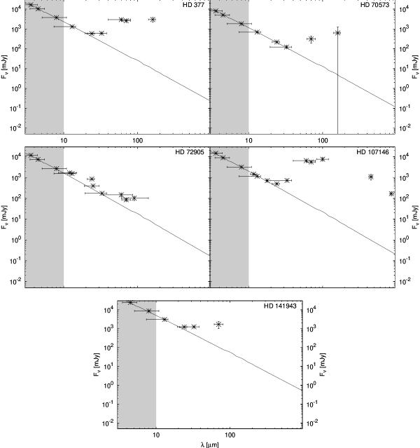
Figure 10.— Observational data for five selected G2V stars. Note that all fluxes have been scaled to the same standard distance of 10pc. Symbols in the left-hand, grey-shaded part of each panel ($\lambda<10\,\mu\hbox{m}$) are IRAC observations. They are used to find an appropriate Hauschildt model to the photosphere (thin solid line), assuming that no excess is already present in the near infrared. Vertical error bars are $1\sigma$ observational uncertainties, taken from the source papers. Horizontal bars indicate the band width of the respective detector.

5.2. Observed excesses

Symbols in Fig. 11 represent the observed excess emission for our sample stars. In the cases where the photospheric subtraction was done in the source papers, we just used the published data points. In the cases where only the total measured flux (star + dust) was given, we proceeded as follows. Three IRAC points ($3.6$, $4.5$, and $8.0\,\mu\hbox{m}$) were fitted by an appropriate NextGen model (Hauschildt et al., 1999), and the resulting photospheric spectrum was subtracted from the fluxes measured at longer wavelengths. As far as the data quality is concerned, the best case is clearly HD 107146, where the data points cover a broad range between $10\,\mu\hbox{m}$ and $1\,\hbox{mm}$. In other cases, the longest wavelengths probed lay at $70$–$160\,\mu\hbox{m}$. As a result, it is sometimes unclear where exactly the excess peaks. This is exemplified by HD 70573 where the $160\,\mu\hbox{m}$ point has a huge error bar.

Figure 11.— Observed (symbols) and modeled (lines) excess emission, scaled to the distance of 10pc. The wavelength range matches the unshaded part of Fig. 10. Here, in contrast to Fig. 10, symbols represent the excess emission. Squares mark the cases where the scaled NextGen model shown on that figure was used to subtract the photosphere. Circles indicate that for these observations the stellar emission was subtracted using photospheric fluxes as given in the respective papers. Dashed lines: two “underlying” SEDs of reference disks (unscaled, i.e. with 10EKBD), one for “cold” excess and one for “warm” excess (except for HD 377 where only cold component is observed). Solid line: a linear combination of two scaled reference SEDs that provides a reasonable fit to the data points (except for HD 377 where a single scaled reference SED is sufficient).

Yet before any comparison with the modeled SEDs, the resulting points in Fig. 11 allow several quick conclusions. Notwithstanding the paucity of long-wavelength data just discussed, in all five systems the excess seems to peak at or slightly beyond $100\,\mu\hbox{m}$, suggesting a “cold EKB” as a source of dust. Additionally, in all systems except for HD 377, a warm emission at $\lambda<20\,\mu\hbox{m}$ seems to be present, implying a closer-in “asteroid belt”.

5.3. Comparison of measured and modeled SEDs

We now proceed with a comparison between the observed dust emission and the modeled emission. We stress that our goal here is not to provide the best fit to the observations possible with our approach, but rather to demonstrate that a set of reference disks modeled in the previous sections can be used to make rough preliminary conclusions about the planetesimal families.

To make such a comparison, we employ the following procedure:

1. For each star, we first look whether only cold or cold + warm excess emission is present. In the former case (HD 377), we fit the data points with a single “cold” reference disk. In the latter case (all other systems), we invoke a two-component model: a close-in $3\,\mbox{AU}$ disk and an appropriate “cold” disk.

2. The location of the “cold” planetesimal belt is chosen according to the peak wavelength of the measured excess: $100\,\mbox{AU}$ (HD 72905 and HD 141943) or $200\,\mbox{AU}$ (HD 377, HD 70573, and HD 107146).

3. We then scale each of the two reference SEDs, “warm” and “cold” (or only one for HD 377) vertically to come to the observed absolute flux. Physically, it necessitates a change in the initial disk mass. However, it is not sufficient to change the initial disk mass by the ratio of the observed flux and the flux from a reference disk. The reason is that a change in the initial mass also alters the rate of the collisional evolution, whereas we need the “right” flux at a fixed time instant, namely the actual age of the system (Tab. 5.1). Therefore, to find the mass modification factor we apply scaling rules, as explained in Appendix A. Specifically, we solve Eq. (A8). In the systems that reveal both warm and cold emission, this is done separately for the inner and outer disk.

The results presented in Fig. 11 with lines show that the modeled SEDs can, generally, reproduce the data points within their error bars. Again, the judgment should take into account the fact that we are just using one or two pre-generated SEDs for a rather coarse grid of reference disks. Much better fits would certainly be possible if we allowed a more exact positioning of parent belts and let additional model parameters vary. Dust opacities, initial distributions of planetesimals’ sizes and orbital elements, as well as their mechanical properties that were fixed in modeling of the collisional outcomes would all be at our disposal for this purpose. Further, more than two-component planetesimal belts could be astrophysically relevant as well, as is the case in our solar system (asteroid belt, different cometary families, various populations in the EKB).

We now come to the interpretation of the fitting results, trying to recover the properties of dust-producing planetesimal belts. Table 5 lists them for all systems. The most important information is the deduced mass and location of the belts.

Table 5Disk properties derived in this study

Star	Component	$M_{\mathrm{disk}}$ [$M_{\oplus}$] 1)	$R_{\mathrm{belt}}$ [AU] 2)	$M_{\mathrm{dust}}$ [$M_{\oplus}$] 3)	$T_{\mathrm{dust}}$ [K] 4)
HD 000377	Outer	$(32)$ 0$32$	$200$	$3.1\times 10^{-2}$	$40$
HD 070573	Inner	$(0.0063)$ 0$0.0046$	$3$	$1.4\times 10^{-7}$	$200$
	Outer	$(2.6)$ 0$2.5$	$200$	$2.0\times 10^{-3}$	$40$
HD 072905	Inner	$(0.054)$ 0$0.019$	$3$	$3.4\times 10^{-8}$	$200$
	Outer	$(0.23)$ 0$0.23$	$100$	$2.1\times 10^{-4}$	$50$
HD 107146	Inner	$(0.039)$ 0$0.023$	$3$	$4.9\times 10^{-7}$	$200$
	Outer	$(47)$ 0$47$	$200$	$4.8\times 10^{-2}$	$40$
HD 141943	Inner	$(0.039)$ 0$0.027$	$3$	$8.0\times 10^{-7}$	$200$
	Outer	$(6.1)$ 0$6.1$	$100$	$5.5\times 10^{-3}$	$50$

Note. — ¹⁾ Initial mass (in parentheses) and the current mass of the whole planetesimal disk (bodies up to $100\,\mbox{km}$ in radius).

²⁾ Location of the parent planetesimal belt.

³⁾ Current mass of “visible” dust (grains up to $1\,\hbox{mm}$ in radius).

⁴⁾ Temperature of cross-section dominating astrosil grains at the location of the parent planetesimal belt, see explanation at Fig. 6.

5.4. Results for hot dust

As far as the hot dust components in four out of five systems are concerned, our results show that these can be explained by “massive asteroid belts” with roughly the lunar mass in bodies up to $\sim 100\,\mbox{km}$ in size, located at $3\,\mbox{AU}$, with a width of $\sim 1\,\mbox{AU}$. However, the quoted distance of inner components — $3\,\mbox{AU}$ — is only due to the fact that this is the smallest disk in our grid. This distance can only be considered as an upper limit: the SEDs seem perfectly compatible with disks as far in as $0.3\,\mbox{AU}$, as suggested for the case of HD 72905 (Wyatt et al., 2007).

What is more, even the very fact that hot excess is real can sometimes be questioned, since it can be mimicked by photospheric emission slightly larger than the assumed values. Indeed, the excess for HD 70573 and HD 72905 at wavelengths around and below $25\,\mu\hbox{m}$ does not exceed 10%, which is comparable with the average calibration uncertainty and therefore has to be considered marginal (Bryden et al., 2006; Hillenbrand et al., 2008). Only in the case of HD 72905, the Spitzer/IRS detection of the $10\,\mu\hbox{m}$ emission from hot silicates provides an independent confirmation that the hot excess is real (Beichman et al., 2006). However, the HD 72905 plot in Fig. 11 makes it obvious that some problems occurred in terms of the photosphere fitting. All data points that we obtained by subtracting the IRAC photospheric fluxes (squares) systematically lie above the data points where a photosphere from the literature was subtracted (circles). The origin of the difference is unclear; on any account, the problem cannot be mitigated by the assumption that an excess is already present at IRAC wavelengths, since this would shift the squares further upwards. Considering the circles to be more trustworthy, the shape of the SED to fit changes. Then a closer-in disk at $\sim 0.3\,\mbox{AU}$ could better reproduce the fluxes in the near and mid infrared, while the outer ring would have to be shifted to a distance somewhat larger than $100\,\mbox{AU}$ in order not to surpass the measured flux at $33~{}\,\mu\hbox{m}$. A problem would arise with the inner disk: at $\sim 0.3\,\mbox{AU}$, the collisional evolution is so rapid that an unrealistically large initial belt mass would be necessary. Similar arguments have led Wyatt et al. (2007) to a conclusion that HD 72905 must be a system at a transient phase rather than a system collisionally evolving in a steady state.

Still, treating the derived sizes and masses of the inner disks as upper limits yields physical implications. Because the collisional evolution close to the star is rapid, such belts must have lost up to two-thirds of their initial mass before they have reached their present age (cf. initial and current mass in Table 5). In the case of HD 70573, the known giant planet with $a=1.76\,\mbox{AU}$ and $e=0.4$ (Setiawan et al., 2007) does not seem to exclude the existence of a dynamically stable planetesimal belt either inside $\sim 1\,\mbox{AU}$ or outside $\sim 3\,\mbox{AU}$.

5.5. Results for cold dust

The estimated parameters of the outer components of the disks suggest “massive and large Kuiper belts”. The radii of the outer rings are larger than the radii derived in previous studies (cf. Table 5.1 and Table 5). This traces back to our using astrosilicate instead of blackbody when calculating the dust emission, so that the same dust temperatures are attained at larger distances (see Fig. 7).

Since one disk in our sample, that of HD 107146, has been resolved, it is natural to compare our derived disk radius with the one obtained from the images. Williams et al. (2004) report an outer border of the system of $150\,\mbox{AU}$ based on submillimeter images. In contrast, Ardila et al. (2004) detected an $85\,\mbox{AU}$-wide ring peaking in density at about $130\,\mbox{AU}$. This is comparable to, although somewhat smaller than, our $200\,\mbox{AU}$ radius. However, moving the outer ring to smaller distances would increase the fluxes in the mid infrared where the SED already surpasses the observations and the other way round in the sub-mm region. The resulting deficiency of sub-mm fluxes, though, could be due to roughness of Mie calculations. As pointed out by Stognienko et al. (1995), an assumption of homogeneous particles typically leads to underestimation of the amount of thermal radiation in the sub-mm region.

Large belt radii imply large masses. Dust masses derived here are by two orders of magnitude larger than previous estimates (cf. Table 5 and Table 5.1). The total masses of the belts we derive range from several to several tens earth masses, to be compared with $\sim 0.1M_{\oplus}$ in the present-day EKB (although there is no unanimity on that point — cf. Stern & Colwell 1997). Note that, as the collisional evolution at $100$–$200\,\mbox{AU}$ is quite slow, whereas the oldest system in our sample is only 420 Myr old, the difference between the initial disk mass and the current disk mass is negligible. Assuming several times the minimum mass solar nebula with a standard surface density of solids $\Sigma\sim 50\,\mbox{g}\,\mbox{cm}^{2}(r/1\,\mbox{AU})^{-3/2}$ (e.g. Hayashi et al., 1985), the mass of solids in the EKB region would be a few tens $M_{\oplus}$; and current models (e.g. Kenyon & Luu, 1999b) successfully accumulate 100 km-sized EKB objects in tens of Myr. However, it is questionable whether the assumed radial surface density profile could extend much farther out from the star. As a result, it is difficult to say, whether a progenitor disk could contain enough solids as far as at $200\,\mbox{AU}$ from the star to form a belt of $30$ to $50M_{\oplus}$.

However, such questions may be somewhat premature. On the observational side, more data are needed, especially at longer wavelengths; for instance, the anticipated Herschel data (PACS at $100/160\,\mu\hbox{m}$ and SPIRE at $250$ to $500\,\mu\hbox{m}$) would help a lot. On the modeling side, a more systematic study is needed to clarify, how strongly various assumptions of the current model (especially the collisional outcome prescription and the material choices) may affect the calculated size distributions of dust, the dust grain temperatures, and the amount of their thermal emission.

At this point, we can only state that in the five systems analyzed (with a possible exception of HD 72905) and with the caveat that available data are quite scarce, the observations are not incompatible with a standard steady-state scenario of collisional evolution and dust production. Of course, other possibilities, such as major collisional breakups (Kenyon & Bromley, 2005; Grigorieva et al., 2007) or events similar to the Late Heavy Bombardment (as suggested, for instance for HD 72905, Wyatt et al. 2007) cannot be ruled out for the inner disks.

6. Summary

Debris disks around main-sequence stars may serve as tracers of planetesimal populations that have accumulated at earlier, protoplanetary and transitional, phases of systems’ evolution, and have not been used up to form planets. However, observations of debris disks are only sensitive to the lowest end of the size distribution. Using dynamical and collisional models of debris disks is the only way to “climb up” the ladder of the collisional cascade, past the ubiquitous $\mu$m-sized grains towards parent bodies and towards the main mass reservoir of the disks.

The main idea of this paper has been to take a grid of planetesimal families (with different initial masses, distances from a central star etc.), to collisionally “generate” debris disks from these families and evolve them with the aid of an elaborated collisional code, and finally, to calculate SEDs for these disks. A comparison/fit of the observed SEDs with the pre-generated SEDs is meant to allow quick conclusions about the properties of the planetesimal belt(s) that maintain one or another observed disk.

Our specific results are as follows:

1. We have produced five reference disks around a G2V star from planetesimal belts at 3, 10, 30, 100, and $200\,\mbox{AU}$ with 10 times the EKB mass density and evolved them for 10 Gyr. With an appropriate scaling rule (Eq. A1), we can translate these results to an arbitrary initial disk mass and any age between 10 Myr and 10 Gyr. Thus, effectively we have a three-parametric set of reference disks (initial mass, location of planetesimal belt, age). For all the disks, we have generated SEDs, assuming astrosilicate (with tests made also for blackbody and amorphous carbon).

2. We have selected five G2V stars with good data (IRAS, ISO/ISOPHOT, Spitzer/IRAC, /IRS, /MIPS, Keck II/LWS, and JCMT/SCUBA) and tested our grid against these data. For all five systems, we have reproduced the data points within the error bars with a linear combination of two disks from the grid (an “asteroid belt” at $3\,\mbox{AU}$ and an outer “Kuiper belt”). This automatically gives us the desired estimates of planetesimals (location, total mass etc.).

3. A comparison of the observational data on the five stars with the grid of models leads us to a conclusion that the cold emission (with a maximum at the far-IR) is compatible with “large Kuiper belts”, with masses in the range 3–50 earth masses and radii of $100$–$200\,\mbox{AU}$. These large sizes trace back to the facts that the collisional model predicts the observed emission to stem from micron-sized dust grains, whose temperatures are well in excess of a blackbody temperature at a given distance from the star (as discussed, e.g., in Hillenbrand et al., 2008). This conclusion is rather robust against variation in parameters of collisional and thermal emission models, and is roughly consistent with disk radii revealed in scattered light images (e.g. HD 107146). Still, quantitative conclusions about the mass and location of the planetesimal belts would significantly depend on (i) the adopted model of collision outcomes (which, in turn, depend on the dynamical excitation of the belts, i.e. on orbital eccentricities and inclinations of planetesimals) and (ii) the assumed grains’ absorption and emission efficiencies. For example, a less efficient cratering (retaining more grains with radii $\sim 10\,\mu\hbox{m}$ in the disk) and/or more “transparent” materials (making dust grains of the same sizes at the same locations colder) would result in “shifting” the parent belts closer to the star.

In future, we plan to extend this study in two directions. First, we will investigate more systematically the influence of the dust composition by trying relevant materials with available optical data rather than astrosilicate; this should be done consistently in the dynamical/collisional and thermal emission models. Second, it is planned to extend this study to stars with a range of spectral classes. This will result in a catalog of disk colors that should be helpful for interpretation of data expected to come, most notably from the Herschel Space Observatory.

Appendix A Scaling rules

1. Dependence of evolution on initial disk mass. Consider a disk with initial mass $M(t=0)\equiv M_{0}$ at a distance $r$ from the star with age $t$. Denote by $F(M_{0},r,t)$ any quantity directly proportional to the amount of disk material in any size regime, from dust grains to planetesimals. In other words, $F$ may equally stand for the total disk mass, the mass of dust, its total cross section, etc. As found by Löhne et al. (2008), there is a scaling rule:

$$F(xM_{0},r,t)=xF(M_{0},r,xt),$$ (A1)

valid for any factor $x>0$. This scaling is an exact property of every disk of particles, provided these are produced, modified and lost in binary collisions and not in any other physical processes.

2. Dependence of evolution on distance. Another scaling rule is the dependence of the evolution timescale on the distance from the star (Wyatt et al., 2007; Löhne et al., 2008). Then

$$F(M_{0},xr,t)\approx F(M_{0},r,t^{-4.3}).$$ (A2)

Unlike Eq. (A1), this scaling is approximate.

3. Dust mass as a function of time. Finally, the third scaling rule found in Löhne et al. (2008) is the power-law decay of the dust mass

$$F(M_{0},r,xt)\approx x^{-\xi}F(M_{0},r,t),$$ (A3)

where $\xi\approx 0.3\ldots 0.4$ (Fig. 12). This scaling is also approximate and, unlike Eq. (A1) and Eq. (A2), only applies to every quantity directly proportional to the amount of dust. In this context, “dust” refers to all objects in the strength rather than gravity regime, implying radii less than about 100 meters. The scaling is sufficiently accurate for disks that are much older than the collisional lifetime of these $100\,\mbox{m}$-sized bodies. This is also seen in Fig. 12: while for the $3\,\mbox{AU}$ disk the power law (A3) sets in after $\ll 1$ Myr, the $200\,\mbox{AU}$ disk needs $\sim 100$ Myr to reach this regime.

Figure 12.— The time evolution of dust mass ($s<1\,\hbox{mm}$) for our five reference disks (thick lines). For comparison, power laws $t^{-\xi}$ with $\xi=0.3$ and $\xi=0.4$ are shown with thin dashed lines.

Note that the “pre-steady-state” phase of collisional evolution may actually require a more sophisticated treatment. Our runs assume initially a power-law size distribution of planetesimals, and an instantaneous start of the collisional cascade at $t=0$. In reality, an initial size distribution is set up by the accretion history of planetesimals and will surely deviate from a single power law. Moreover, at a certain phase cratering and destruction of objects may increasingly come into play simultaneously with ceasing, yet ongoing accretion; the efficiencies and timescales of these processes will be different for different size ranges and different spatial locales in the disk (e.g. Davis & Farinella, 1997; Kenyon & Luu, 1998, 1999a, 1999b).

The usefulness of these scaling rules can be illustrated with the following examples.

Example 1. Assuming now $F$ to be the total amount of dust, from Eqs. (A1)–(A3) one finds

$$F(xM_{0},yr,t)\approx x^{1-\xi}y^{4.3\xi}F(M_{0},r,t).$$ (A4)

Our choice of reference disks (different distances, but the same volume density) implies $x=y^{3}$. The normal optical optical depth $\tau\propto F/r^{2}$ scales as

$$\tau(y^{3}M_{0},yr,t)\approx y^{1+1.3\xi}\tau(M_{0},r,t).$$ (A5)

Therefore, once a steady-state is reached ($\xi\approx 0.3...0.4$), a $y$ times more distant planetesimal belt gives rise to a $y^{1+1.3\xi}$ times optically thicker disk. This explains, in particular, why in Fig. 4 any $100\,\mbox{AU}$ ring is $\approx 30$ times optically thicker than the co-eval $10\,\mbox{AU}$ one.

Example 2. Since the distance $r$ in Eqs. (A1) and (A3) is kept fixed, $F$ in these equations can also denote the radiation flux, emitted by a disk at a certain wavelength. Let $F_{o}(t)$ be the observed flux from a disk of age $t$. Imagine a model of a disk of the same age with an initial mass $M_{0}$ predicts a flux $F(M_{0},t)$ which is by a factor $A$ lower than the observed one:

$$F_{o}(t)=AF(M_{0},r,t).$$ (A6)

Our goal is to find the “right” initial mass, i.e. a factor $B$ such that

$$F_{o}(t)=F(BM_{0},r,t).$$ (A7)

With the aid of Eq. (A1), this can be rewritten as

$$F_{o}(t)=BF(M_{0},r,Bt).$$ (A8)

Eq. (A3) gives now

$$F_{o}(t)\approx BF(M_{0},r,t)B^{-\xi}=B^{1-\xi}F(M_{0},r,t),$$ (A9)

whence

$$B\approx A^{1/(1-\xi)}.$$ (A10)

For instance, a 10 times higher flux at a certain age requires a 27–46 times larger initial disk mass if $\xi=0.3\ldots 0.4$.

Although this rule is convenient for quick estimates, it should be used with caution. As described above, the value of $\xi$ at the beginning of collisional evolution (which lasts up to 100 Myr for the $200\,\mbox{AU}$ belt) can be much smaller — close to zero or even negative — than the “normal” $\xi=0.3\ldots 0.4$. For this reason, we prefer to use only the first scaling rule, Eq. (A1). Therefore, instead of applying Eq. (A10), we find $B$ by solving Eq. (A8) numerically with a simple iterative routine. It is this way Fig. 11 was constructed.

References

- Ardila et al. (2004) Ardila, D. R., et al. 2004, ApJ, 617, L147
- Artymowicz (1997) Artymowicz, P. 1997, Ann. Rev. Earth Planet. Sci., 25, 175
- Aumann et al. (1984) Aumann, H. H., et al. 1984, ApJ, 278, L23
- Beichman et al. (2005) Beichman, C. A., et al. 2005, ApJ, 622, 1160
- Beichman et al. (2006) Beichman, C. A., et al. 2006, ApJ, 639, 1166
- Bohren & Huffman (1983) Bohren, C. F., & Huffman, D. R. 1983, Absorption and Scattering of Light by Small Particles (Wiley and Sons: New York – Chichester – Brisbane – Toronto – Singapore)
- Bryden et al. (2006) Bryden, G., et al. 2006, ApJ, 636, 1098
- Burns et al. (1979) Burns, J. A., Lamy, P. L., & Soter, S. 1979, Icarus, 40, 1
- Carpenter et al. (2005) Carpenter, J. M., Wolf, S., Schreyer, K., Launhardt, R., & Henning, T. 2005, AJ, 129, 1049
- Davis & Farinella (1997) Davis, D. R., & Farinella, P. 1997, Icarus, 125, 50
- Dohnanyi (1969) Dohnanyi, J. S. 1969, J. Geophys. Res., 74, 2531
- Durda & Dermott (1997) Durda, D. D., & Dermott, S. F. 1997, Icarus, 130, 140
- Gladman et al. (2001) Gladman, B., et al. 2001, AJ, 122, 1051
- Grigorieva et al. (2007) Grigorieva, A., Artymowicz, P., & Thébault, P. 2007, A&A, 461, 537
- Hahn & Malhotra (2005) Hahn, J. M., & Malhotra, R. 2005, AJ, 130, 2392
- Hauschildt et al. (1999) Hauschildt, P., Allard, F., & Baron, E. 1999, ApJ, 512, 377
- Hayashi et al. (1985) Hayashi, C., Nakazawa, K., & Nakagawa, Y. 1985, in Protostars and Planets II, ed. D. C. Black & M. S. Matthews, 1100–1153
- Hillenbrand et al. (2008) Hillenbrand, L. A., et al. 2008, ApJ, 677, 630
- Kenyon & Bromley (2005) Kenyon, S. J., & Bromley, B. C. 2005, AJ, 130, 269
- Kenyon & Luu (1998) Kenyon, S. J., & Luu, J. X. 1998, AJ, 115, 2136
- Kenyon & Luu (1999a) —. 1999a, AJ, 118, 1101
- Kenyon & Luu (1999b) —. 1999b, ApJ, 526, 465
- Krivov et al. (2006) Krivov, A. V., Löhne, T., & Sremčević, M. 2006, A&A, 455, 509
- Krivov et al. (2000) Krivov, A. V., Mann, I., & Krivova, N. A. 2000, A&A, 362, 1127
- Krivov et al. (2005) Krivov, A. V., Sremčević, M., & Spahn, F. 2005, Icarus, 174, 105
- Laor & Draine (1993) Laor, A., & Draine, B. T. 1993, ApJ, 402, 441
- Löhne et al. (2008) Löhne, T., Krivov, A. V., & Rodmann, J. 2008, ApJ, 673, 1123
- Meyer et al. (2004) Meyer, M. R., et al. 2004, ApJS, 154, 422
- Moór et al. (2006) Moór, A., et al. 2006, ApJ, 644, 525
- Najita & Williams (2005) Najita, J., & Williams, J. P. 2005, ApJ, 635, 625
- Rhee et al. (2007) Rhee, J. H., Song, I., Zuckerman, B., & McElwain, M. 2007, ApJ, 660, 1556
- Rieke et al. (2005) Rieke, G. H., et al. 2005, ApJ, 620, 1010
- Setiawan et al. (2007) Setiawan, J., et al. 2007, ApJ, 660, L145
- Siegler et al. (2007) Siegler, N., et al. 2007, ApJ, 654, 580
- Spangler et al. (2001) Spangler, C., Sargent, A. I., Silverstone, M. D., Becklin, E. E., & Zuckerman, B. 2001, ApJ, 555, 932
- Stern & Colwell (1997) Stern, S. A., & Colwell, J. E. 1997, ApJ, 490, 879
- Stognienko et al. (1995) Stognienko, R., Henning, T., & Ossenkopf, V. 1995, A&A, 296, 797
- Su et al. (2006) Su, K. Y. L., et al. 2006, ApJ, 653, 675
- Thébault & Augereau (2007) Thébault, P., & Augereau, J.-C. 2007, A&A, 472, 169
- Thébault et al. (2003) Thébault, P., Augereau, J.-C., & Beust, H. 2003, A&A, 408, 775
- Trilling et al. (2008) Trilling, D. E., et al. 2008, ApJ, 674, 1086
- Trilling et al. (2007) Trilling, D. E., et al. 2007, ApJ, 658, 1289
- Williams et al. (2004) Williams, J. P., et al. 2004, ApJ, 604, 414
- Wolf & Hillenbrand (2003) Wolf, S., & Hillenbrand, L. A. 2003, ApJ, 596, 603
- Wyatt (2005) Wyatt, M. C. 2005, A&A, 433, 1007
- Wyatt et al. (2007) Wyatt, M. C., et al. 2007, ApJ, 658, 569