Theories and models of superconducting state Magnetic properties Non-Fermi-liquid ground states, electron phase diagrams and phase transitions in model systems

Competitions of magnetism and superconductivity in FeAs-based materials

Abstract

Using the numerical unrestricted Hartree-Fock approach, we study the ground state of a two-orbital model describing newly discovered FeAs-based superconductors. We observe the competition of a $(0,\pi)$ mode spin-density wave and the superconductivity as the doping concentration changes. There might be a small region in the electron-doping side where the magnetism and superconductivity coexist. The superconducting pairing is found to be spin singlet, orbital even, and mixed s_xy + d${}_{x^{2}-y^{2}}$ wave (even parity).

The newly discovered FeAs-based superconductors [1, 2] have attracted lots of experimental[3, 4, 5, 7, 8, 9, 6] and theoretical [10, 11, 12, 16, 13, 14, 15, 17, 18, 19, 20, 21, 22, 23, 24, 30, 31, 25, 26, 27, 28, 29, 32, 33, 34, 38, 35, 36, 37, 39] interests. Experimentally, the superconducting transition temperature, up to now, can be as high as 56K[5, 4, 6]. Spin-density wave order of $(0,\pi)$ mode was observed in the parent compound LaOFeAs, but vanishes at high temperature (above 150K) and large doping region[4, 9]. However, unlike the cuprate high-Tc superconductors whose parent compound is an insulator, LaOFeAs is a semimetal[4, 10]. The observed magnetic dependence of the specific heat as well as the results of nuclear magnetic resonate suggest the presence of gapless nodal lines on the Fermi surface[3]. Theoretically, the transition temperature estimated based on the electron-phonon coupling seems unlikely to explain the observed superconductivity, thus suggesting these materials might be unconventional and non-electron-phonon mediated [16]. The local-density-approximation (LDA) calculations show that the density of state near the Fermi surfaces of the parent compound LaOFeAs are dominated by iron’s 3d electrons[10, 11, 12, 13, 14, 15]. These observations imply that the multi-orbital effects play a key role in these new family of high-Tc superconductors. Though irons in LaOFeAs have five orbitals and ten bands, some groups proposed that it is sufficient to consider only a few of them, say $d_{xz}$ and $d_{yz}$ orbitals for a minimal two-band model or may include $d_{xy}$ orbital for a three-band model, to reproduce qualitatively the LDA Fermi surface topology[20, 21, 22, 23, 24, 25, 26, 27, 28, 29]. The spin-density-wave (SDW) of $(0,\pi)$ mode of the parent compound LaOFeAs has been interpreted due to the superexchange interaction between the next-nearest neighboring sites, which leads to an effective $J_{1}-J_{2}$ model defined on a two-dimensional lattice [30, 31, 18, 25, 35]. Alternatively, the SDW mode was also attributed to the nesting of Fermi surface [4, 12, 21, 27, 28, 33, 34]. On the other hand, despite of the pairing mechanism being unclear, some groups [36, 37, 39, 38] have addressed the classification of various superconducting states of the systems with two orbitals based on group theory.

In this paper, we study the competition between superconductivity and magnetism, as well as the superconducting pairing symmetry in the FeAs-based materials. Based on a recently proposed two-orbital model, we introduce the superconducting pairing into the Hamiltonian from which various pairing possibility can be constructed. Then we study the ground state property by using the unrestricted Hartree-Fock approach. We start with random values for all possible order parameters and let the self-consistent equations converge to the final solution. We find that for the parent compound, there exists a $(0,\pi)$ mode spin-density-wave. When doping is introduced, either by electron or hole, superconductivity appears with the disappearance of the magnetism, and there is a small overlap in electron-doping region where the magnetism and superconductivity might coexist. Therefore, these is a competition between the two orders. In the superconducting region, a careful scrutiny reveals that the pairing symmetry of the superconductivity might involve spin singlet, orbital symmetric, and mixed s_xy+d${}_{x^{2}-y^{2}}$ wave (even parity).

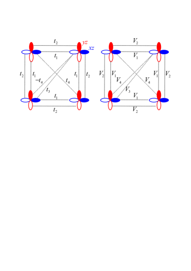
Figure 1: (color online) The schematic illustration for the hopping parameters and the attractive interaction parameters of the two-orbital $d_{xz}-d_{yz}$ model on a square lattice.

In order to simplify the calculation, we adopt the two-band model of the Fe subsystem defined on the principle plane, as suggested by Raghu etal [23], as a starting model for discussing the interplay between magnetism and superconductivity. While there are arguments as to whether the minimum model should consist of three orbitals, we expect no qualitative difference to appear within our calculation framework. There are two “$d_{xz}$, $d_{yz}$” orbitals on each site. The left plot of fig. 1 shows all possible hoping processes between neighboring sites and orbitals based on the tight binding approximations. Phenomenologically, we use the following mean-field Hamiltonian,

$$H = H_{0}+H_{SC}+H_{I},$$ (1)

$$H_{0} = \sum_{k\sigma}\psi_{k\sigma}^{{\dagger}}\left[\epsilon_{k}\tau_{0}+\gamma_{k}\tau_{1}+\xi_{k}\tau_{3}\right]\psi_{k\sigma},$$ (2)

$$H_{I} = -U\sum_{i,\beta}m_{i}^{\beta}\left(C_{i,\uparrow}^{\beta{\dagger}}C_{i,\uparrow}^{\beta}-C_{i,,\downarrow}^{\beta{\dagger}}C_{i,\downarrow}^{\beta}\right)$$ (3)

$$+\sum_{i,\sigma}\left(U^{\prime}+\frac{J_{H}}{4}\right)\left(\rho_{i,\sigma}^{a}n_{i,-\sigma}^{b}-\frac{1}{2}\rho_{i,\sigma}^{a}\rho_{i,-\sigma}^{b}\right)$$

$$+\sum_{i,\sigma}\left(U^{\prime}-\frac{J_{H}}{4}\right)\left(\rho_{i,\sigma}^{a}n_{i,-\sigma}^{b}-\frac{1}{2}\rho_{i,\sigma}^{a}\rho_{i,\sigma}^{b}\right)$$

$$+\frac{J_{H}}{2}\left(\sum_{i,\alpha,\beta}\Delta_{i}^{\alpha\beta}C_{i,\sigma}^{\alpha}C_{i,-\sigma}^{\beta}+h.c.-|\Delta_{i}^{\alpha\beta}|^{2}\right)$$

The physical meaning of all parameters and operators in the Hamiltonian are presented in order. $H_{0}$ is the noninteracting term [23] with

$$\psi_{k,\sigma} = (C_{\sigma}^{a}(k),C_{\sigma}^{b}(k)),$$ (4)

$$\epsilon_{k} = -(t_{1}+t_{2})(\cos k_{x}+\cos k_{y})-4t_{3}\cos k_{x}\cos k_{y}-\mu,$$ (5)

$$\gamma_{k} = -4t_{4}\sin k_{x}\sin k_{y},$$ (6)

$$\xi_{k} = -(t_{1}-t_{2})(\cos k_{x}-\cos k_{y}),$$ (7)

and $\alpha,\beta=a(xz),b(yz)$ label orbitals, and $\tau$ is the Pauli matrix for $xz$ and $yz$ orbitals [The superscript $a(b)$ is specified to “$d_{xz}(d_{yz})$” orbital hereafter]. $H_{I}$ is a Hartree-Fock decomposition of the on-site interaction term, result from

$$H_{I} = U\sum_{i,\beta}n_{i,\uparrow}^{\beta}n_{i,\downarrow}^{\beta}$$ (8)

$$+\sum_{i}\left[U^{\prime}n_{i}^{a}n_{i}^{b}-J_{H}\left(\mathbf{S}_{i}^{a}\cdot\mathbf{S}_{i}^{b}+\mathbf{\eta}_{i}^{a}\cdot\mathbf{\eta}_{i}^{b}\right)\right]~{},$$

in which $J_{H}$ denotes the Hunds rule coupling, $U(U^{\prime})$ the on-site Coulomb interaction between electrons on the same (distinct) bands, and $S_{i}^{\beta+}=C_{i,\uparrow}^{\beta{\dagger}}C_{i,\downarrow}^{\beta},S_{i}^{\beta z}=(n_{i,\uparrow}^{\beta}-n_{i,\downarrow}^{\beta})/2,\eta_{i}^{\beta+}=C_{i,\uparrow}^{\beta{\dagger}}C_{i,\downarrow}^{\beta{\dagger}},\eta_{i}^{\beta z}=(n_{i}^{\beta}-1)/2$. Both $S$ and $\eta$ satisfy SU(2) Lie algebra, and $U=U^{\prime}+J_{H}$ [40]. Local order parameters $m_{i}^{\beta}$ and $\rho_{i,\sigma}^{\beta}$ are defined as

$$m_{i}^{\beta} = \frac{1}{2}\left(\langle n_{i,\uparrow}^{\beta}\rangle-\langle n_{i,\downarrow}^{\beta}\rangle\right),$$ (9)

$$\rho_{i,\sigma}^{\beta} = \langle n_{i,\sigma}^{\beta}\rangle.$$ (10)

Respecting to the fact that underline mechanism for superconducting properties observed in cuprates is controversial, we are not in the position to discuss what mechanism is for the FeAs-based superconductivity. Instead, our purpose is to address the interplay between superconductivity and magnetism so we will start from the assumption that electrons on neighboring sites pair in the following form

$$H_{SC} = -V\sum_{i,\delta,\beta,\sigma}\left[\Delta_{i,\delta,\sigma}^{\beta}C_{i+\delta,\sigma}^{\beta}C_{i,-\sigma}^{\beta}+h.c.-\left|\Delta_{i,\delta,\sigma}^{\beta}\right|^{2}\right]$$

$$-V\sum_{i,\delta^{\prime},\alpha,\beta,\sigma}\left[\Delta_{i,\delta^{\prime},\sigma}^{\alpha\beta}C_{i+\delta^{\prime},\sigma}^{\beta}C_{i,-\sigma}^{\alpha}+h.c.-\left|\Delta_{i,\delta^{\prime},\sigma}^{\alpha\beta}\right|^{2}\right]~{},$$

where $V$ accounts for the attractive interaction between electrons on neighboring sites, $\delta(\delta^{\prime})$ denotes the (next) nearest neighboring sites [fig. 1 (Right)].

Figure 2: (color online) The superconducting order, the magnetism order, and doping as function of the chemical potential.

The mean-field Hamiltonian is quadratic and can be diagonalized numerically by solving self-consistent equations following standard procedure. In our numerical calculations, we set $t_{1}=-1$, $t_{2}=1.3$, $t_{3}=t_{4}=-0.85$, and $J_{H}=1.4\sim 2.0$ in unit of $|t_{1}|$, according the LDA calculations, and vary other parameters to explore the ground-state prosperities. Solving such multi-variable nonlinear equations is a very complicated and time consuming task because of many quantities under iteration: we have 8 independent $\Delta_{i,\delta,\sigma}^{\beta}$s, 16 $\Delta_{i,\delta^{\prime},\sigma}^{\alpha\beta}$s, 4 $\Delta_{i}^{\alpha\beta}$s, and 4 density parameters $\rho_{i,\sigma}^{\beta}$s for each site, and for a $L\times L$-site system, so the total number of iterated quantities is $32L^{2}$. The reason for us to perform the unrestricted Hartree-Fock calculations, rather than the restricted ones (where one would have much reduced number of self-consistent variables), is to obtain unbiased ground state pairing and magnetic ordering patterns.

To address the competition between the magnetism and superconductivity. We first define the superconducting and magnetic order parameters in $k$-space as follows

$$\Delta_{k}^{\alpha\beta} = \frac{1}{N}\sum_{jl}e^{i(j-l)k}\Delta_{j,l}^{\alpha\beta},$$ (12)

$$m_{k} = \frac{1}{\sqrt{N}}\sum_{j,\beta}e^{ijk}m_{j}^{\beta}.$$ (13)

Then we calculate the magnetic order and superconducting order parameter defined as,

$$\Delta = \frac{1}{N}\sum_{\alpha,\beta,k}\left|\Delta_{k}^{\alpha\beta}\right|,$$ (14)

$$\left|m\right| = \frac{1}{N}\sum_{j,\beta}\left|m_{j}^{\beta}\right|.$$ (15)

Fig. 2 shows the main results of the doping ratio, magnetic order, and superconducting order as a function of the chemical potential for a typical parameter set $U=3.4$, $V=0.9$, and $J_{H}=1.5$. Note that paring driving force usually comes from a second order process so it is expected that $V$ is smaller than any other renormalized Coulomb interactions. We firstly observe that there is a flat region in the doping as the chemical potential varies. Though the position of the flat is a little above the half-filling for finite size lattices we studied, it will tend to the half-filling as the system size increases. From fig. 2(b), we notice that the magnetic order is nonzero around the half-filling. This observation is consistent with experimental results that the parent compound shows magnetic order without doping. The dominant magnetic order is $(\pi,0)$, or $(0,\pi)$ SDW. Once electrons or holes are doped into the parent compound, the magnetic order is gradually suppressed to zero, and superconducting order appears, as shown in fig. 2(a). At half-filling, the superconductivity is absent. In experiments, the parent compound is a poor metal without superconductivity. Therefore, our numerical results are consistent with the experimental results qualitatively. As electrons are doped into the material, the superconducting order appears at a certain doing concentration. As the doping concentration becomes larger, it will disappear again. Similar behavior also occurs in the hole doping region. One of the most interesting observation is that, in the electrons doping region, both the magnetism and superconducting orders do not vanish at a small region. Therefore, the magnetism and superconductivity are not exclusive with each other. So though there is a competition between two orders, the magnetism and superconductivity might coexist in a very narrow region.

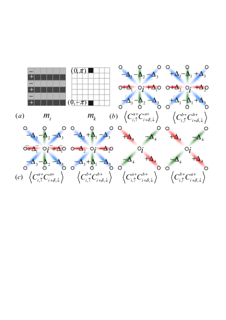
Figure 3: (color online) (a) $(0,\pi)$ spin density wave at half-filling. (b)Pairing structures of the (next) nearest neighboring sites in electron doped region. (c) Pairing structures of the (next) nearest neighboring sites in hole doped region. Here $\Delta_{i},i=1,2,3,4$ denote simply the pairing amplitude which will be shown in main text.

Next we check the magnetic order and pair symmetry of the superconductivity. The order parameters defined in $k$-space, i.e. eq. (12) and eq. (13), can help us to learn the details of magnetic order and pairing symmetry. In this work, we consider three typical cases below.

Case A (undoped compound): We consider the magnetic property of the parent compound for the parameter set

$$U=3.5,V=1.0,J_{H}=1.5,\mu=3.3.$$ (16)

Here, we set the initial value of local magnetization at random and let self-consistent equations converge. We observe that the dominant magnetization patten in $k$ space include either $(0,\pi)$ or $(\pi,0)$. Fig. 3(a) shows the magnetic ordering in both the real and $k$-space. In the real space, the compound shows a stripe-like phase which represents the spin collinear order. The local magnetization are $\pm 0.227$ for light and dark gray respectively. This observation is consistent with the experimental results of the magnetic properties in undoped case. If we make a Fourier transformation, we find a spin-density wave of $(0,\pi)$ mode in $k$ space. Therefore, $m_{k}=0.227$ at $(0,\pm\pi)$, and zero elsewhere. Here, we would like to point out that $(\pi,0)$ mode can also be observed even we started iteration with initial conditions consist with of other order parameters. Moreover, our numerical simulations show that the magnetic order dominates in the low-doping region.

Case B (electron doping): Electron doping typically occurs at

$$U=3.5,V=1.0,J_{H}=1.5,\mu=3.7~{},$$ (17)

where the solution converges at 13.8% electron doping. In this large doping region, the anti-ferromagnetism of the parent compound are suppressed by superconductivity. The intra-orbital pairing structures of the (next) nearest neighboring sites are illustrated in fig. 3(b) schematically. In fig 3(b), $\Delta_{1}=\langle C_{i,\uparrow}^{a\dagger}C_{i+x,\downarrow}^{a\dagger}\rangle=0.04824$, $\Delta_{2}=\langle C_{i,\uparrow}^{a\dagger}C_{i+y,\downarrow}^{a\dagger}\rangle=0.05176$ and $\Delta_{3}=\langle C_{i,\uparrow}^{a\dagger}C_{i+x+y,\downarrow}^{a\dagger}\rangle=0.03584$. While the inter-orbital pairings are found to be zero within numerical accuracy. Hence from numerical results, the nearest-neighbor intra-band pairing belongs to d${}_{x^{2}-y^{2}}$-wave symmetry ($\cos k_{x}-\cos k_{y}$), while the next-nearest-neighbor intra-band pairing looks like an extended s_xy-wave ($\cos k_{x}\cos k_{y}$), and there is no inter-band (next) nearest neighboring pairing. In addition, the superconducting order parameters in $k$ space obey the following relation

$$\left\langle C_{k,\sigma}^{\beta{\dagger}}C_{-k,-\sigma}^{\alpha{\dagger}}\right\rangle=\left\langle C_{-k,\sigma}^{\beta{\dagger}}C_{k,-\sigma}^{\alpha{\dagger}}\right\rangle,$$ (18)

which concludes that the pairing symmetry involves spin singlet, orbital symmetric, and mixed s_xy + d${}_{x^{2}-y^{2}}$ wave (even parity).

Case C (hole doping): Hole doping typically occurs at

$$U=3.5,V=1.0,J_{H}=1.5,\mu=2.8~{},$$ (19)

where the solution converges at 11.5% hole doping and without spin density wave. The first two graphs of fig. 3(c) show that the (next) nearest intra-band pairing are still mixed s_xy + d${}_{x^{2}-y^{2}}$ wave. The pairing amplitude are $\Delta_{1}=0.04525$, $\Delta_{2}=0.01864$ and $\Delta_{3}=0.03444$. Moreover, unlike case B, the next nearest inter-band pairing interactions are not too small to ignore. As illustrated by the last two graphs in fig. 3(c), the signs of the order parameters in real space denote the d-wave inter-band pairing structures. The pairing amplitude is $\Delta_{4}=\langle C_{i,\uparrow}^{a\dagger}C_{i+x+y,\downarrow}^{b\dagger}\rangle=0.00185$. We also notice that the relation $\left\langle C_{k,\sigma}^{\beta{\dagger}}C_{-k,-\sigma}^{\alpha{\dagger}}\right\rangle=\left\langle C_{-k,\sigma}^{\beta{\dagger}}C_{k,-\sigma}^{\alpha{\dagger}}\right\rangle$ still holds in the hole doping region. Therefore, the pairing symmetry are the same as in case B.

In summary, applying the numerical unrestricted Hartree-Fock approach to a two-orbital model, we have studied the competition between magnetism and superconductivity, as well as superconducting pair symmetry in the newly discovered FeAs-based superconductors. We found that there does exist competitions between magnetic and superconducting orders. Despite of this, the magnetism and superconductivity may still coexist in a small region. In order to find the possible magnetic order and pairing symmetry. We further studied three different cases, corresponding to undoped, electron doped, and hole doped, respectively. We found that, around updoped region, the parent compound shows a spin-density wave of $(0,\pi)$ mode, while in both the electron and hole doped region, the superconducting pairing symmetry involves spin singlet, orbital symmetric, and mixed s_xy + d${}_{x^{2}-y^{2}}$ wave(even parity). We noticed also that the result is somehow different from that of numerical renormalization calculation [33]. This might be due to the different range of interactions, as well as different approach used. Finally, we remark that although we used the two-orbital model, suggested by previous studies, as the starting model in our calculation, conclusions drawn should not be altered qualitatively when more orbitals are included in our approach.

- [1] \NameKamihara Y., Hiramatsu H., Hirano M., Kawamura R., Yanagi H., Kamiya T. Hosono H. \REVIEWJ. Am. Chem. Soc.13020083296.
- [2] \NameTakahashi H., Igawa K., Arii K, Kamihara Y., Hirano M., Hosono H. \REVIEWNature4532008376.
- [3] \NameWen H. H., Mu G., Fang L., Yang H. Zhu X. Y. \REVIEWEurophys. Lett.82200817009; \NameMu G., Zhu X. Y., Fang L., Shan L., Ren C., Wen H. H. \REVIEWChin.Phys.Lett.2520082221-2224.
- [4] \NameDong J., Zhang H. J., Xu G., Li Z., Li G., Hu W. Z., Wu D., Chen G. F., Dai X., Luo J. L., Fang Z. Wang N. L. arXiv:0803.3426; \NameChen G. F., Li Z., Wu D., Li G., Hu W. Z., Dong J., Zheng P., Luo J. L., Wang N. L. \REVIEWPhys. Rev. Lett.1002008247002;\NameChen G. F., Li Z., Wu D., Dong J., Li G., Hu W. Z., Zheng P., Luo J. L., Wang N. L. \REVIEWChin. Phys. Lett.2520082235.
- [5] \NameRen Z. A., Yang J., Lu W., Yi W., Shen X. L., Li Z. C., Che G. C., Dong X. L., Sun L. L., Zhou F., Zhao Z. X. \REVIEWEurophys. Lett.82200857002; \NameRen Z. A., Lu W., Yang J., Yi W., Shen X. L., Li Z. C., Che G. C., Dong X. L., Sun L. L., Zhou F., Zhao Z. X. \REVIEWChin. Phys. Lett.2520082215.
- [6] \NameLi L., Li Y., Ren Z., Lin X., Luo Y., Zhu Z., He M., Xu X., Cao G., Xu Z. arXiv:0806.1675;\NameRen Z., Zhu Z., Jiang S., Xu X., Tao Q., Wang C., Feng C., Cao G., Xu Z. arXiv:0806.2591.
- [7] \NameChen X. H., Wu T., Wu G., Liu R. H., Chen H., Fang D. F. \REVIEWNature4532008376.
- [8] \NameOu H. W., Zhao J. F., Zhang Y., Shen D. W., Zhou B., Yang L. X., He C., Chen F., Xu M., Wu T., Chen X. H., Chen Y., Feng D. L. \REVIEWChin. Phys. Lett.2520082225.
- [9] \NameCruz C., Huang Q., Lynn J. W., Li J. Y., Ratcliff II W., Zarestky J. L., Mook H. A., Chen G. F., Luo J. L., Wang N. L., Dai P. C. \REVIEWNature4532008899.
- [10] \NameSingh D. J. Du M. H. \REVIEWPhys. Rev. Lett.1002008237003.
- [11] \NameHaule K., Shim J. H. Kotliar G. \REVIEWPhys. Rev. Lett.1002008226402.
- [12] \NameXu G., Ming W., Yao Y., Dai X., Zhang S. C. Fang Z. \REVIEWEurophys. Lett.82200867002.
- [13] \NameMazin I. I., Singh D. J., Johannes M. D. Du M. H. arXiv:0803.2740.
- [14] \NameCao C., Hirschfeld P. J. Cheng H. P. \REVIEWPhys. Rev. B772008220506.
- [15] \NameMa F. J. Lu Z. Y. arXiv:0803.3286.
- [16] \NameBoeri L., Dolgov O. V., Golubov A. A. arXiv:0803.2703.
- [17] \NameMa F. J. Lu Z. Y. arXiv:0803.3286.
- [18] \NameMa F. J., Lu Z. Y., Xiang T. arXiv:0804.3370.
- [19] \NameLv J. P. Chen Q. H. arXiv:0805.0632.
- [20] \NameDai X., Fang Z., Zhou Y., Zhang F. C. arXiv:0803.3982.
- [21] \NameHan Q., Chen Y., Wang Z. D. \REVIEWEurophys. Lett.82200837007.
- [22] \NameLi T. arXiv:0804.0536.
- [23] \NameRaghu S., Qi X. L., Liu C. X., Scalapino D. J. Zhang S. C. \REVIEWPhys. Rev. B772008220503(R).
- [24] \NameLee P. A. Wen X. G. arXiv:0804.1739.
- [25] \NameSi Q. M.Abrahams E. arXiv:0804.2480.
- [26] \NameWeng Z. Y. arXiv:0804.3228.
- [27] \NameYao Z. J., Li J. X. Wang Z. D. arXiv:0804.4166.
- [28] \NameQi X. L., Raghu S., Liu C. X., Scalapino D. J. Zhang S. C. arXiv:0804.4332 (2008).
- [29] \NameDaghofer M., Moreo A., Riera J. A., Arrigoni E. Dagotto E. arXiv:0805.0148.
- [30] \NameYao D. X. Carlson E. W. arXiv:0804.4115.
- [31] \NameYildirim T. arXiv:0804.2252.
- [32] \NameLi J. Wang Y. P. \REVIEWChin. Phys. Lett.2520082232.
- [33] \NameWang F., Zhai H., Ran Y., Vishwanath A., Lee D. H. arXiv:0805.3343.
- [34] \NameRan Y., Wang F., Zhai H., Vishwanath A., Lee D. H. arXiv:0805.3535.
- [35] \NameSeo K., Bernevig B. A., Hu J. P. arXiv:0805.2958.
- [36] \NameWang Z. H., Tang H., Fang Z. Dai X. arXiv:0805.0736.
- [37] \NameWan Y. Wang Q. H. arXiv:0805.0923.
- [38] \NameShi J. R. arXiv:0806.0259.
- [39] \NameZhou Y., Chen W. Zhang F. C. arXiv:0806.0712.
- [40] \NameCastellani C. Natoli C. R., Ranninger J. \REVIEWPhys. Rev. B1819784945.