Sampling constraints in average: The example of Hugoniot curves

Abstract

We present a method for sampling microscopic configurations of a physical system distributed according to a canonical (Boltzmann-Gibbs) measure, with a constraint holding in average. Assuming that the constraint can be controlled by the volume and/or the temperature of the system, and considering the control parameter as a dynamical variable, a sampling strategy based on a nonlinear stochastic process is proposed. Convergence results for this dynamics are proved using entropy estimates. As an application, we consider the computation of points along the Hugoniot curve, which are equilibrium states obtained after equilibration of a material heated and compressed by a shock wave.

Statistical physics provides a way to obtain macroscopic quantities starting from systems described at the microscopic level. In this framework, the state of the system is described by some probability measure, the precise choice of the measure depending on the invariant quantities at hand. A fundamental statistical ensemble for instance is the microcanonical ensemble which is generated by the ergodic limit of the Hamiltonian dynamics, and corresponds to isolated systems. Another classical ensemble is the canonical ensemble, for which the temperature is constant. In one possible derivation of the associated probability measure, the statistical entropy is maximized subject to the constraint that the average energy of the system is fixed, and the temperature is related to the Lagrange multiplier of the former constraint [4]. More generally, it may be of interest to consider ensembles such that some constraint (not only the energy) is satisfied on average. The challenge is to have an explicit description of the corresponding thermodynamic ensemble in terms of the associated probability measure. In an effort to define the statistical distributions sampled by methods aiming at satisfying constraints on average, we first reformulate here the problem of sampling with constraints satisfied in average in the context of the canonical ensemble.

The paper is organized as follows. In Section 1, we formulate precisely the problem of sampling canonical ensembles with a constraint fixed in average, giving a specific example and recalling some previous sampling strategies. In Section 2, we present a nonlinear stochastic process with a feedback term depending on the expectation of the constraint, who admits the target measure as a stationary state. We also prove the convergence to this target measure using entropy estimates for initial data not too far from the limiting state (the proofs being presented in Section 4). In Section 3, we discuss the numerical implementation, proposing a single trajectory discretization, and use the method to compute the Hugoniot curve of Argon.

1 Mathematical formulation of the problem

Consider a microscopic system of $N$ particles in a space of dimension $d=3$, described by their positions $q=(q_{1},\dots,q_{N})$ and momenta $p=(p_{1},\dots,p_{N})$, with associated mass matrix $M={\rm Diag}(m_{1},\dots,m_{N})$, and interacting through a potential $V$. Periodic boundary conditions are used, and the particles then stay in a domain $\mathcal{D}=L_{x}\mathbb{T}\times L_{y}\mathbb{T}\times L_{z}\mathbb{T}$ ($\mathbb{T}$ denoting the one-dimensional torus $\mathbb{R}/\mathbb{Z}$). The volume of the domain is denoted by $|\mathcal{D}|$. The phase-space $\Omega$ is

$$\Omega=\mathcal{M}\times\mathbb{R}^{3N}=\mathcal{D}^{N}\times\mathbb{R}^{3N}.$$

The central quantity describing the system is the Hamiltonian

$$H(q,p)=\sum_{i=1}^{N}\frac{p_{i}^{2}}{2m_{i}}+V(q_{1},\dots,q_{N}).$$ (1)

The canonical measure associated with the Hamiltonian (1) has a density [4]

$$\pi_{\mathcal{D},T}(q,p)=\frac{1}{Z_{\mathcal{D},T}}\textrm{e}^{-\beta H(q,p)},\qquad\beta^{-1}=k_{\rm B}T,$$ (2)

where $k_{\rm B}$ is the Boltzmann constant, and the partition function $Z_{\mathcal{D},T}$ is a normalization factor so that (2) is indeed a probability measure:

$$Z_{\mathcal{D},T}=\int_{\Omega}\textrm{e}^{-\beta H(q,p)}\,dq\,dp.$$ (3)

We have indicated explicitly the dependence of the canonical measure (2) and the partition function (3) on the temperature $T$ and the domain $\mathcal{D}$. Average thermodynamic properties of the system can be computed as averages of functions of the microscopic variables (the so-called observables) with respect to the canonical measure at a temperature $T$ and for a given simulation box $\mathcal{D}$:

$$\langle A\rangle_{\mathcal{D},T}=\int_{\Omega}A(q,p)\,\pi_{\mathcal{D},T}(q,p)\,dq\,dp.$$ (4)

Canonical simulations are performed at a fixed volume. However, this is an ill-defined notion since there are infinitely many simulations domains having the same volume. In practice, the shape of the simulation box (for instance cubic) is kept constant, and the volume is changed using a scaling of the positions $q$. We will in any case assume in the sequel that the knowledge of the volume $|\mathcal{D}|$ is enough to characterize the domain $\mathcal{D}$.

1.1 Equilibrium sampling

In most cases, equilibrium sampling at a fixed temperature and for a fixed geometry $\mathcal{D}$ is performed (see [8, 1, 7] for references on sampling methods), and the output of the simulation is the average property $\langle A\rangle_{\mathcal{D},T}$. This can be done for instance by means of ergodic results for the Langevin dynamics

$$\left\{\begin{array}[]{ccl}dq_{t}&=&\displaystyle M^{-1}p_{t}\,dt,\\[5.0pt] dp_{t}&=&\displaystyle-\nabla V(q_{t})\,dt-\xi M^{-1}p_{t}\,dt+\sqrt{2\xi k_{\rm B}T}\,dW_{t},\\[5.0pt] \end{array}\right.$$ (5)

where $\xi>0$ is physically interpreted as a friction, and $W_{t}$ is a standard $3N$-dimensional Brownian motion. Under mild assumptions on the potential $V$ [7],

$$\lim_{\tau\to+\infty}\frac{1}{\tau}\int_{0}^{\tau}A(q_{t},p_{t})\,dt=\langle A\rangle_{\mathcal{D},T}\quad\mathrm{a.s.}$$

for almost all initial conditions. When the observable $A$ considered depends only on the positions of the particles (which is not too restrictive since the momentum contribution of many observables can be explicitly computed), the overdamped Langevin dynamics

$$dq_{t}=-\nabla V(q_{t})\,dt+\sqrt{2k_{\rm B}T}\,dW_{t},$$

may be used as well since (again, under some assumptions on the potential [7])

$$\lim_{\tau\to+\infty}\frac{1}{\tau}\int_{0}^{\tau}A(q_{t})\,dt=\frac{\displaystyle\int_{\mathcal{M}}A(q)\,\textrm{e}^{-\beta V(q)}\,dq}{\displaystyle\int_{\mathcal{M}}\textrm{e}^{-\beta V(q)}\,dq}=\langle A\rangle_{\mathcal{D},T}\quad\mathrm{a.s.}$$

1.2 Satisfying constraints in average

The inverse sampling problem is sometimes of interest: given some value $A_{0}$ of an average property (for instance, some average energy), what should the temperature and/or the volume of the system be? Answering this question allows to sample configurations of the system canonically distributed and satisfying the constraint $A(q,p)=A_{0}$ in average (in the sense that $\langle A\rangle_{\mathcal{D},T}=A_{0}$). In the sequel we will focus on constraints depending on $T$, and therefore drop the mention of the volume in the notation of the canonical averages when it is not relevant. Constraints on the volume can be handled similarly. Moreover, upon replacing $A$ by $A-A_{0}$, it can be assumed that $A_{0}=0$, so that the problem under investigation is

$$\framebox{$\text{Find }T\text{ such that }\langle A\rangle_{T}=0.$}$$ (6)

In order to have a well-defined problem (and possibly upon replacing $A$ by $-A$), it is assumed that

Assumption 1.

There exists an interval $I^{A}_{T}=[T^{A}_{\mathrm{min}},T^{A}_{\mathrm{max}}]$ (with $T^{A}_{\mathrm{min}}>0$), a temperature $T^{\ast}\in(T^{A}_{\mathrm{min}},T^{A}_{\mathrm{max}})$, and constants $a,\alpha>0$ such that

$$\forall T\in I_{T}^{A},\quad\langle A\rangle_{T}=0\Leftrightarrow T=T^{\ast},$$

and

$$\forall T\in I_{T}^{A},\quad\alpha\leq\frac{\langle A\rangle_{T}-\langle A\rangle_{T^{\ast}}}{T-T^{\ast}}\leq a.$$

The assumption on the observable is satisfied as soon as $T\mapsto\langle A\rangle_{T}$ is locally $\mathrm{C}^{1}$ around a value $T^{*}$ such that $\langle A\rangle_{T^{\ast}}=0$ and $\left.\partial_{T}\left(\langle A\rangle_{T}\right)\right|_{T^{\ast}}>0$. An example is illustrated in Figure 2 for the test case considered in Section 3.2.

1.3 Some examples

1.3.1 Hugoniot curves

The method presented in this paper is illustrated on Hugoniot sampling (see Section 3.2). The variations of macroscopic quantities across a shock interface are governed by the Rankine-Hugoniot relations, which relate the jumps of the quantities under investigation (pressure, density, velocities) to the velocity of the shock front. The third Rankine-Hugoniot conservation law for the Euler equation governing the hydrodynamic evolution of the fluid reads (macroscopic quantities are denoted by curly letters)

$${\cal E}-{\cal E}_{0}-\frac{1}{2}({\cal P}+{\cal P}_{0})(\mathcal{V}_{0}-\mathcal{V})=0.$$ (7)

In this expression, ${\cal E}$ is the internal energy of the fluid, ${\cal P}$ its pressure, and $\mathcal{V}$ its volume. The subscript $0$ refers to the initial state, the other quantities are evaluated at a shocked state, after equilibration. The Hugoniot curve corresponds to all the possible states satisfying (7). In practice, it is computed by considering shocks of different strengths, inducing various compressions.

A reference temperature $T_{0}$ and a simulation cell $\mathcal{D}_{0}$, for instance $\mathcal{D}_{0}=(L_{0}\mathbb{T})^{3}$, characterize the equilibrium state before the shock. In numerical experiments, the compression rate

$$c=\frac{|\mathcal{D}|}{|\mathcal{D}_{0}|}$$

is varied from 1 to some maximal compression rate $0<c_{\text{max}}<1$, so that $\mathcal{D}=(c^{1/3}L_{0}\mathbb{T})^{3}$ when the compression is isotropic. Since all macroscopic quantities arising in the hydrodynamic equations are obtained relying on some local thermodynamic equilibrium assumption, (7) can be reformulated at the microscopic level using statistical mechanics. For a given compression rate c,

$$\langle H\rangle_{|\mathcal{D}|,T}-\langle H\rangle_{|\mathcal{D}_{0}|,T_{0}}-\frac{1}{2}(\langle P\rangle_{|\mathcal{D}|,T}+\langle P\rangle_{|\mathcal{D}_{0}|,T_{0}})(|\mathcal{D}_{0}|-|\mathcal{D}|)=0,$$

where the pressure observable for a domain $\mathcal{D}$ is

$$P(q,p)=\frac{1}{3|\mathcal{D}|}\sum_{i=1}^{N}\frac{p_{i}^{2}}{2m_{i}}-q_{i}\cdot\nabla_{q_{i}}V(q).$$

Notice that we indicate explicitly the dependence on the volumes for clarity, though the initial and final volumes are given. The final temperature $T$ is the only unknown, and it satisfies

$$\left\langle H(q,p)-\langle H\rangle_{|\mathcal{D}_{0}|,T_{0}}+\frac{1}{2}(P(q,p)+\langle P\rangle_{|\mathcal{D}_{0}|,T_{0}})(1-c)|\mathcal{D}_{0}|\right\rangle_{|\mathcal{D}|,T}=0.$$

Introducing the Hugoniot observable (parametrized by the compression parameter $c$)

$$A_{c}(q,p)=H(q,p)-\langle H\rangle_{|\mathcal{D}_{0}|,T_{0}}+\frac{1}{2}(P(q,p)+\langle P\rangle_{|\mathcal{D}_{0}|,T_{0}})(1-c)|\mathcal{D}_{0}|,$$ (8)

the Hugoniot problem can be reformulated as

$$\text{For a given compression }c_{\text{max}}\leq c\leq 1,\text{ find }T\text{ such that }\langle A_{c}\rangle_{c|\mathcal{D}_{0}|,T}=0.$$ (9)

The compression rate $c$ parametrizes a curve in the $(P,T)$ diagram, called the Hugoniot curve. Note that this curve does not correspond to a thermodynamic path.

Since shock waves propagate in one direction (for instance parallel to the $x$ axis), anisotropic version of the Hugoniot problem are of interest. In this case, the compression acts in the $x$ direction only, and $\mathcal{D}=cL_{0}\mathbb{T}\times(L_{0}\mathbb{T})^{2}$. The average pressure $P$ is replaced by the $P_{xx}$ component of the pressure tensor:

$$P_{xx}(q,p)=\frac{1}{|\mathcal{D}|}\sum_{i=1}^{N}\frac{p_{i,x}^{2}}{2m_{i}}-q_{i,x}\nabla_{q_{i,x}}V(q),$$

where $q_{i,x},p_{i,x}$ denote respectively the $x$ components of the position and momenta of the $i$-th particle, and the observable $A_{c}$ is replaced by

$$A_{xx,c}(q,p)=H(q,p)-\langle H\rangle_{|\mathcal{D}_{0}|,T_{0}}+\frac{1}{2}(P_{xx}(q,p)+\langle P_{xx}\rangle_{|\mathcal{D}_{0}|,T_{0}})(1-c)|\mathcal{D}_{0}|.$$

The $xx$ component of the initial pressure tensor $\langle P_{xx}\rangle_{|\mathcal{D}_{0}|,T_{0}}$ may be replaced by the average pressure $\langle P\rangle_{|\mathcal{D}_{0}|,T_{0}}$ when the initial state is isotropic.

1.3.2 A more general case

More generally, Hamiltonians depending on some external parameter$~{}\lambda$ can be considered, with associated observables $A$ controlled by the value of $\lambda$. For instance, $\lambda$ could be the intensity of a magnetic field for a spin system, and $A$ the total magnetization. The problem is then to find $\lambda$ such that

$$\langle A\rangle_{\mathcal{D},T,\lambda}=\frac{\displaystyle\int_{\Omega}A(q,p)\,\textrm{e}^{-\beta H_{\lambda}(q,p)}\,dq\,dp}{\displaystyle\int_{\Omega}\textrm{e}^{-\beta H_{\lambda}(q,p)}\,dq\,dp}=0,$$

the volume $\mathcal{D}$ and the temperature $T$ being fixed.

1.4 Previous sampling algorithms

1.4.1 Newton’s method

An obvious sampling strategy to compute the zero of the function $T\mapsto F(T)=\langle A\rangle_{T}$ is to resort to Newton’s algorithm. It is expected that such an approach converges in a few steps if the function $F$ is well behaved. However, the derivative $F^{\prime}(T)$ often involves the computation of covariances, which are known to require long sampling times to be reliably computed. For instance, when trying to sample configurations with the average energy fixed, $A=H$ and

$$\partial_{T}(\langle H\rangle_{T})=\frac{1}{k_{\rm B}T^{2}}(\langle H^{2}\rangle_{T}-\langle H\rangle_{T}^{2}).$$

A way to bypass this difficulty is to estimate numerically the derivative by computing averages at two temperatures $T+\Delta T$ and $T-\Delta T$ around the temperature $T$, and to approximate the derivative as

$$\partial_{T}(\langle A\rangle_{T})\simeq\frac{\langle A\rangle_{T+\Delta T}-\langle A\rangle_{T-\Delta T}}{2\Delta T}.$$

This method is robust, and is indeed used in Monte-Carlo studies of the Hugoniot problem [5]. It requires however very carefully converged canonical samplings in order to have a numerical estimate of the derivative not polluted by sampling errors.

1.4.2 New thermodynamic ensembles

It would be better to have a more automatic procedure, consisting for instance of a single molecular dynamics trajectory. In this case, convergence needs only be checked once, and the simulation can be runned longer if needed. This was the motivation for the Hugoniostat method [15], which can be extended to any constraint whose values are controlled by the temperature $T$. The idea of the method is to satisfy approximately the constraint $A(q,p)=0$ at all times. To this end, a convenient dynamics in the Nosé-Hoover fashion [17, 13] is postulated:

$$\left\{\begin{array}[]{ccl}\dot{q}&=&M^{-1}p,\\ \dot{p}&=&-\nabla V(q)-\xi p,\\[5.0pt] \dot{\xi}&=&\displaystyle\nu^{2}\frac{A(q,p)}{A_{\rm ref}},\\ \end{array}\right.$$ (10)

where $\nu>0$ is homogeneous to a frequency, and $A_{\rm ref}$ is some reference value of the observable. When the instantaneous value of the observable is lower than the target value $0$, $\xi$ decreases and the friction is reduced, so that the (kinetic) temperature in the system, and therefore the average value of the observable, can increase; while the friction increases for too large values of the observable, and so, energy is removed from the system and the temperature decreases. This feedback process ensures indeed that values of the observable around the target value are sampled, though it is unclear how the temperature of the system is defined. For computational purposes, the temperature is defined as the average kinetic temperature along the trajectory.

The numerical results obtained with the dynamics (10) are correct for the Hugoniot problem since they are in agreement with numerical results from shock wave simulations, see [15] for more precisions. However, the question of the choice of the frequency $\nu$ in (10) remains, as usual for Nosé-like dynamics. More importantly, from a fundamental viewpoint, an unpleasant feature is that the thermodynamic ensemble (i.e. the probability measure on phase space) associated with the dynamics used is not known. It may be defined as the ergodic limit of the dynamics, for a given set of parameters and initial conditions. Even if this is possible, it is unclear whether the limiting measure depends on the parameters used and on the initial conditions, or not. The problem remains even if the Nosé-Hoover part of the above dynamics is replaced by a Langevin dynamics (for which ergodicity results are usually easier to state) or any dynamics ergodic for the canonical measure (see [7] for references on the convergence properties of some sampling methods). For instance, the usual Langevin dynamics (5) at temperature $T$ may be extended to the case of constraints satisfied in average by considering the temperature as a dynamical variable:

$$\left\{\begin{array}[]{ccl}dq_{t}&=&M^{-1}p_{t}\,dt,\\ dp_{t}&=&-\nabla V(q_{t})\,dt-\xi M^{-1}p_{t}\,dt+\sqrt{2\xi k_{\rm B}T_{t}}\,dW_{t},\\[5.0pt] dT_{t}&=&-\displaystyle\nu\frac{A(q_{t},p_{t})}{A_{\rm ref}}\,T_{\text{ref}}\,dt,\\ \end{array}\right.$$ (11)

where $\nu>0$ is again some frequency, and $T_{\text{ref}}$, $A_{\rm ref}$ are reference values of the temperature and the observable respectively. When the instantaneous value of the observable is too low, the temperature is increased, while it is decreased when it is too large. For computational purposes, the temperature may be defined as the time average of $T_{t}$ over a trajectory, though, as for the dynamics (10), the meaning of this quantity is unclear since there is no obvious definition of the thermodynamic temperature within the ensemble generated by the dynamics (11). Therefore, (11) is not satisfactory.

2 A nonequilibrium sampling strategy

2.1 General algorithm

To solve the sampling problem (6), we consider the temperature as a variable, so that the system is described by the variables $(q,p,T)$. The idea is that the update of the current configuration $(q,p)$ is governed by a dynamics consistent with canonical sampling at the instantaneous temperature $T(t)$ (such as Nosé-Hoover methods [17, 13], Metropolis-Hastings algorithms [16, 11], Langevin or overdamped Langevin dynamics,…), while the temperature is updated depending on the current estimate of $\langle A\rangle_{T(t)}$. For instance, consider the following system when the underlying dynamics is of overdamped Langevin type:

$$\left\{\begin{array}[]{ccl}dq_{t}&=&\displaystyle-\nabla V(q_{t})\,dt+\sqrt{2k_{\rm B}T(t)}\,dW_{t},\\[5.0pt] T^{\prime}(t)&=&\displaystyle-\gamma\,\mathbb{E}(A(q_{t})),\\ \end{array}\right.$$ (12)

or

$$\left\{\begin{array}[]{ccl}dq_{t}&=&\displaystyle M^{-1}p_{t}\,dt,\\[5.0pt] dp_{t}&=&\displaystyle-\nabla V(q_{t})\,dt-\xi M^{-1}p_{t}\,dt+\sqrt{2\xi k_{\rm B}T(t)}\,dW_{t},\\[5.0pt] T^{\prime}(t)&=&\displaystyle-\gamma\,\mathbb{E}(A(q_{t},p_{t})),\\ \end{array}\right.$$ (13)

when the underlying dynamics is of Langevin type. In both cases, $\gamma>0$ determines the time scale of the temperature feedback term, and $W_{t}$ is a standard $3N$-dimensional Brownian motion. To prove mathematical results, it is convenient to use (elliptic) overdamped Langevin dynamics, since the associated Fokker-Planck equation describing the evolution of the law of the process $q_{t}$ is parabolic. However, we will use the hypoelliptic Langevin dynamics in the numerical applications presented in Section 3 since this dynamics is usually a more efficient sampling device [7]. When the overdamped Langevin dynamics is used, the canonical measure $\mu_{T}$ in position space has the density

$$\mu_{T}(q)=\frac{1}{Z_{T}}\exp\left(-\frac{V(q)}{k_{\mathrm{B}}T}\right),\qquad Z_{T}=\int_{\mathcal{M}}\exp\left(-\frac{V(q)}{k_{\mathrm{B}}T}\right)\,dq,$$

and averages with respect to the canonical measure $\mu_{T}$ are still denoted $\displaystyle\langle A\rangle_{T}=\int_{\mathcal{M}}A(q)\,\mu_{T}(q)\,dq$.

2.1.1 Motivation

The dynamics (12) and (13) can be motivated as follows. If the configurations followed adiabatically the temperature changes, the positions $q_{t}$ (and possibly the momenta $p_{t}$) would be distributed canonically at the temperature $T(t)$ at all times, and

$$T^{\prime}(t)=-\gamma\,\langle A\rangle_{T(t)}.$$

Assumption (1) then shows that $T(t)\to T^{\ast}$. Indeed, starting from a temperature $T(0)$ in the interval $I_{T}^{A}$ of Assumption 1, it is easily seen that $t\mapsto(T(t)-T^{\ast})^{2}$ is a decreasing function: if $T(t)\in I_{T}^{A}$, then

$$\partial_{t}\left[\frac{1}{2}(T(t)-T^{\ast})^{2}\right] = -\gamma\langle A\rangle_{T(t)}(T(t)-T^{\ast})=-\gamma(\langle A\rangle_{T(t)}-\langle A\rangle_{T^{\ast}})(T(t)-T^{\ast})$$

$$\leq -\gamma\alpha(T(t)-T^{\ast})^{2}\leq 0,$$

and so, $T(t)\in I_{T}^{A}$ whenever $T(0)\in I_{T}^{A}$. Suppose for instance $T(0)>T^{\ast}$. Then $T(t)\geq T^{\ast}$ at all times and, with Assumption 1,

$$-\gamma a(T(t)-T^{\ast})\leq T^{\prime}(t)=-\gamma(\langle A\rangle_{T(t)}-\langle A\rangle_{T^{\ast}})\leq-\gamma\alpha(T(t)-T^{\ast}).$$

Gronwall’s lemma then implies

$$T^{\ast}+(T(0)-T^{\ast})\,\mathrm{e}^{-a\gamma t}\leq T(t)\leq T^{\ast}+(T(0)-T^{\ast})\,\mathrm{e}^{-\alpha\gamma t},$$

which shows the convergence $T(t)\to T^{\ast}$ as $t\to+\infty$.

Of course, the positions are not canonically distributed at all times. The hope is that, even if equilibrium is not maintained at all times, the dynamics can still converge if the typical time arising in the temperature update is small enough compared to the typical relaxation time of the dynamics, so that the spatial relaxation happens gradually, as $T(t)$ approaches $T^{\ast}$. This statement is made precise in Section 2.2 (see Theorems 2 and 3). From a practical viewpoint, the interest of such a strategy is that, if the dynamics is started off equilibrium (for instance at a temperature much larger than the target temperature $T^{\ast}$), then it is not necessary to fully relax the system at the starting temperature (as is the case for instance for the Newton method presented in Section 1.4.1), and so, computational savings may be anticipated. The convergence proof is however only valid for initial data not too far from the stationary state. This is related to the fact that the temperature has to remain positive, and so, it is not possible in general to start arbitrarily far from equilibrium.

Remark 1 (Possible extensions).

A nonlinear temperature feedback may be considered as well:

$$T^{\prime}(t)=-\gamma f\left(\mathbb{E}(A(q_{t}))\right),$$ (14)

under some assumptions on the function $f$ – see Remark 3 for more precisions.

It is also possible to use a time varying parameter $\gamma(t)$ for the temperature update, for instance smaller at the beginning of the simulation, and then larger once the equilibrium state is approached. The proofs presented below may be extended to this case provided $\gamma(t)$ remains in a properly chosen interval around an admissible value of $\gamma$ (as given by Theorems 2 and 3).

2.1.2 Partial differential equation reformulation

The nonlinear partial differential equation (PDE) reformulation of the dynamics (12) is

$$\left\{\begin{array}[]{ccl}\partial_{t}\psi&=&\displaystyle k_{\rm B}T(t)\,\nabla\cdot\left[\mu_{T(t)}\nabla\left(\frac{\psi}{\mu_{T(t)}}\right)\right]=k_{\rm B}T(t)\,\Delta\psi+\nabla\cdot(\psi\nabla V),\\[10.0pt] T^{\prime}(t)&=&\displaystyle-\gamma\int_{\mathcal{M}}A(q)\psi(t,q)\,dq,\\ \end{array}\right.$$ (15)

where the periodic function $q\in\mathcal{M}\mapsto\psi(t,q)$ is the law of the process $q_{t}$ at time $t$.

The PDE (15) clearly admits $(T^{\ast},\mu_{T^{\ast}})$ as a stationary solution. Since the first equation of (15) is of parabolic type, standard techniques may be used to prove the (short time) existence of a unique solution, for initial conditions smooth enough, and under the following smoothness assumptions on the potential and the observable:

Assumption 2.

The observable $A\in\mathrm{C}^{3}(\mathcal{M})$ and $V\in\mathrm{C}^{2}(\mathcal{M})$.

In particular, the observable is bounded, which is important to ensure that the temperature remains positive. Indeed, if this was not the case, it would be possible to obtain negative temperatures arbitrarily fast by concentrating the initial density $\psi^{0}$ around singularities of the observable. The boundedness of $A$ ensures some delay in the feedback.

Theorem 1.

When Assumption 2 holds, and for a given initial condition $(T^{0},\psi^{0})$, with $T^{0}>0$ and

$$\psi^{0}\in\mathrm{H}^{2}(\mathcal{M}),\qquad\psi^{0}\geq 0,\qquad\int_{\mathcal{M}}\psi^{0}=1,$$

there exists a time $\displaystyle\tau\geq\frac{T^{0}}{2\gamma\|A\|_{\infty}}>0$ such that (15) has a unique solution $(T,\psi)$ with $T\in\mathrm{C}^{1}([0,\tau],\mathbb{R})$ and $\psi\in\mathrm{C}^{0}([0,\tau],\mathrm{H}^{2}(\mathcal{M}))$. Moreover, $\psi\geq 0$, and $\psi>0$ when $\psi^{0}>0$.

The proof is presented in Section 4.1. The regularity assumptions on $\psi^{0}$ is not too restrictive since an arbitrary initial condition $\widetilde{\psi}^{0}\in\mathrm{L}^{2}(\mathcal{M})$ can be evolved using an overdamped Langevin dynamics at $T^{0}$ for some time $\tau_{\rm init}>0$ before turning on the temperature feedback term. Then, the resulting distribution $\psi^{0}=\widetilde{\psi}(\tau_{\rm init},\cdot)$ is smooth thanks to the regularizing properties of the parabolic Fokker-Planck equation. To obtain the uniqueness and existence of the solution at all times, it is necessary to show that the temperature remains isolated from 0. This is proved in Section 2.2 together with the convergence to the stationary state, under certain conditions on the initial entropy (see Theorems 2 and 3).

2.2 Convergence results for initial conditions close to the fixed-point

To study the convergence of the nonlinear dynamics (15) under its PDE form, entropy methods can be used (see for instance the review papers [10, 2]). The total entropy of the system is the sum of a spatial entropy $E(t)$, related to the distribution of configurations at time $t$, and a temperature term:

$$\mathcal{E}(t)=E(t)+\frac{1}{2}(T(t)-T^{\ast})^{2},$$

with

$$E(t)=\int_{\mathcal{M}}h\left(f\right)\mu_{T(t)},\qquad f=\frac{\psi}{\mu_{T(t)}}.$$

Notice that the spatial entropy $E(t)$ measures the distance of the law of the process $\psi$ to the instantaneous equilibrium measure $\mu_{T(t)}$, and not to some fixed reference measure. Two classical choices for the spatial entropy are the relative entropy distance (which corresponds to $h(x)=x\ln x-x+1\geq 0$) and $\mathrm{L}^{2}$ distances ($\displaystyle h(x)=\frac{1}{2}(x-1)^{2}$). We present convergence results for both cases (see Theorems 2 and 3), which are very similar in spirit, but involve different functional settings for the initial conditions. In particular, the conditions on the initial condition are more stringent in Theorem 3, but the assumptions to be verified by the potential are less demanding.

The convergence is ensured provided $\mathcal{E}(t)\to 0$ as $t\to+\infty$. This implies in particular $T(t)\to T^{\ast}$, and also

$$\|\psi(t,\cdot)-\mu_{T^{\ast}}\|_{\mathrm{L}^{1}}\leq\|\psi(t,\cdot)-\mu_{T(t)}\|_{\mathrm{L}^{1}}+\|\mu_{T(t)}-\mu_{T^{\ast}}\|_{\mathrm{L}^{1}}\leq c_{h}\,E(t)+\|\mu_{T(t)}-\mu_{T^{\ast}}\|_{\mathrm{L}^{1}}\to 0,$$

where the constant $c_{h}$ depends on the chosen entropy density $h$ (using a Csizár-Kullback inequality for relative entropy estimates, and a Cauchy-Schwarz inequality for $\mathrm{L}^{2}$ entropies). The strategy of the proof is to obtain a Gronwall inequality for $\mathcal{E}(t)$. This ensures also that the temperature is well defined (in particular, $T(t)>0$ at all times). Indeed, if the total entropy is decreasing, then $|T(t)-T^{\ast}|$ is bounded by $\sqrt{2\mathcal{E}(0)}$, and the temperature remains isolated from 0 for initial data whose total entropy is small enough.

In the proofs presented in Section 4, estimates on the derivative of the spatial entropy are a key element. Since

$$\partial_{t}\mu_{T(t)}=\frac{T^{\prime}(t)}{k_{\mathrm{B}}T(t)^{2}}\left(V-\left\langle V\right\rangle_{T(t)}\right)\,\mu_{T(t)},$$

and thus

$$\partial_{t}f=\frac{\partial_{t}\psi}{\mu_{T(t)}}-\frac{T^{\prime}(t)}{k_{\mathrm{B}}T(t)^{2}}\left(V-\left\langle V\right\rangle_{T(t)}\right)\,f,$$

it holds

$$\frac{dE(t)}{dt} = \int_{\mathcal{M}}h^{\prime}(f)\,\partial_{t}f\,\mu_{T(t)}+\int_{\mathcal{M}}h(f)\partial_{t}\mu_{T(t)}$$

$$= \int_{\mathcal{M}}h^{\prime}(f)\,\partial_{t}\psi+\frac{T^{\prime}(t)}{k_{\mathrm{B}}T(t)^{2}}\int_{\mathcal{M}}\left[h(f)-h^{\prime}(f)\,f\right]\,\left(V-\left\langle V\right\rangle_{T(t)}\right)\,\mu_{T(t)}$$

$$= k_{\rm B}T(t)\,\int_{\mathcal{M}}h^{\prime}(f)\,\nabla\cdot\left[\mu_{T(t)}\nabla\left(\frac{\psi}{\mu_{T(t)}}\right)\right]+\frac{T^{\prime}(t)}{k_{\mathrm{B}}T(t)^{2}}\int_{\mathcal{M}}\left[h(f)-h^{\prime}(f)\,f\right]\,\left(V-\left\langle V\right\rangle_{T(t)}\right)\,\mu_{T(t)}$$

$$= -k_{\rm B}T(t)\,\int_{\mathcal{M}}h^{\prime\prime}(f)\,\left|\nabla f\right|^{2}\,\mu_{T(t)}+\frac{T^{\prime}(t)}{k_{\mathrm{B}}T(t)^{2}}\int_{\mathcal{M}}\left[h(f)-h^{\prime}(f)\,f\right]\,\left(V-\left\langle V\right\rangle_{T(t)}\right)\,\mu_{T(t)}.$$

In view of Theorem 1, the above manipulations (in particular the integrations by parts) can be performed, at least for $t$ small enough. The proofs of convergence are based on the following strategy: The first term in the above equality is bounded by $-\rho E(t)$ for some $\rho>0$ using a functional inequality (logarithmic Sobolev inequality (LSI) or a Poincaré inequality, depending on the functional setting), while the remainder is shown to be small for $\gamma$ small enough thanks to the temperature derivative factor.

2.2.1 Relative entropy estimates

This case corresponds to the choice $h(x)=x\ln x-x+1$. In addition of Assumption 2, we suppose that

Assumption 3.

There exists an interval $I^{\mathrm{LSI}}_{T}=[T^{\mathrm{LSI}}_{\mathrm{min}},T^{\mathrm{LSI}}_{\mathrm{max}}]$ (with $T^{\mathrm{LSI}}_{\mathrm{min}}>0$ and $T^{\mathrm{LSI}}_{\mathrm{min}}<T^{\ast}<T^{\mathrm{LSI}}_{\mathrm{max}}$) such that the family of measures $\{\mu_{T}\}_{T\in I^{\mathrm{LSI}}_{T}}$ satisfies a logarithmic Sobolev inequality (LSI) with a uniform constant $1/\rho$, namely

$$\int_{\mathcal{M}}h(f)\mu_{T}\leq\frac{1}{\rho}\int_{\mathcal{M}}\frac{|\nabla f|^{2}}{f}\,\mu_{T}.$$

A LSI holds for instance in the following cases: when the potential $V$ satisfies a strict convexity condition of the form ${\rm Hess}(V)\geq\nu\,{\rm Id}$ with $\nu>0$ (as a special case of the Bakry and Emery criterion [3]), or when the measure $\mu_{T}$ is a tensorization of measures satisfying a LSI (see Gross [9]). Moreover, when a LSI with constant $\rho$ is satisfied by $Z_{V}^{-1}\,{\rm e}^{-V(q)}\,dq$, then $Z_{V+W}^{-1}\,{\rm e}^{-(V(q)+W(q))}\,dq$ (with $W$ bounded) satisfies a LSI with constant $\tilde{\rho}=\rho\,{\rm e}^{\inf W-\sup W}$. This property expresses some stability with respect to bounded pertubations (see Holley and Stroock [12]). In particular, a LSI is verified for the canonical measure associated with smooth potentials on a compact state space (as is the case here). The uniformity of the constant can be ensured by restricting the temperatures to a finite interval isolated from 0.

Theorem 2.

Consider a potential $V$ and an observable $A$ such that Assumptions 1 and 3 hold, and an initial data $(T^{0},\psi^{0})$ with $\psi^{0}\in\mathrm{H}^{2}(\mathcal{M})$, $\psi^{0}\geq 0$, $\displaystyle\int_{\mathcal{M}}\psi^{0}=1$, and associated entropy $\mathcal{E}(0)\leq\mathcal{E}^{\ast}$, where

$$\mathcal{E}^{\ast}=\inf\left\{\frac{1}{2}(T_{\mathrm{min}}^{A}-T^{\ast})^{2},\frac{1}{2}(T_{\mathrm{max}}^{A}-T^{\ast})^{2},\frac{1}{2}(T_{\mathrm{min}}^{\mathrm{LSI}}-T^{\ast})^{2},\frac{1}{2}(T_{\mathrm{max}}^{\mathrm{LSI}}-T^{\ast})^{2}\right\}.$$

Then, there exists $\gamma_{0}>0$ such that, for all $0<\gamma\leq\gamma_{0}$, (15) has a unique solution $(T,\psi)\in\mathrm{C}^{1}([0,\tau],\mathbb{R})\times\mathrm{C}^{0}([0,\tau],\mathrm{H}^{2}(\mathcal{M}))$ for all $\tau\geq 0$, and the entropy converges exponentially fast to zero: There exists $\kappa>0$ (depending on $\gamma$) such that

$$\mathcal{E}(t)\leq\mathcal{E}(0)\exp(-\kappa t).$$

In particular, the temperature remains positive at all times: $T(t)\geq\min(T_{\mathrm{min}}^{\mathrm{LSI}},T_{\mathrm{min}}^{A})>0$, and it converges exponentially fast to $T^{*}$.

Remark 2.

The proof shows that the convergence rate $\kappa$ is larger when (i) $\mathcal{E}(0)$ is lower (the dynamics starts closer from the fixed point and/or closer from a spatial local equilibrium); (ii) $\alpha$ is larger (the slope of the function $T\mapsto\langle A\rangle_{T}$ is steeper around the target value $T^{\ast}$); (iii) $\rho$ is larger (the relaxation of the spatial distribution of configurations at a fixed temperature happens faster).

2.2.2 $\mathrm{L}^{2}$ estimates

This case corresponds to the choice $\displaystyle h(x)=\frac{1}{2}(x-1)^{2}$. In this section, in addition of Assumption 2 (and instead of Assumption 3), we suppose that

Assumption 4.

There exists an interval $I^{\mathrm{Poincare}}_{T}=[T^{\mathrm{Poincare}}_{\mathrm{min}},T^{\mathrm{Poincare}}_{\mathrm{max}}]$ (with $T^{\mathrm{Poincare}}_{\mathrm{min}}>0$ and $T^{\mathrm{Poincare}}_{\mathrm{min}}<T^{\ast}<T^{\mathrm{Poincare}}_{\mathrm{max}}$) such that the family of measures $\{\mu_{T}\}_{T\in I^{\mathrm{Poincare}}_{T}}$ satisfies a Poincaré inequality with a uniform constant $1/\rho$, namely

$$\int_{\mathcal{M}}h(f)\mu_{T}\leq\frac{1}{\rho}\int_{\mathcal{M}}|\nabla f|^{2}\,\mu_{T}.$$

Recall that LSI imply Poincaré inequalities (see for instance [2]), so that the second part of Assumption 4 is less demanding than the second part of Assumption 3, and is verified for instance for smooth potentials on compact state spaces. A result analogous to Theorem 2 can be stated upon defining another bound on the initial entropy (recall that bounds in $\mathrm{L}^{2}$ entropy are more demanding than bounds in relative entropy [2]).

Theorem 3.

Consider a potential $V$ and an observable $A$ such that Assumptions 1 and 4 hold, and an initial data $(T^{0},\psi^{0})$ with $\psi^{0}\in\mathrm{H}^{2}(\mathcal{M})$, $\psi^{0}\geq 0$, $\displaystyle\int_{\mathcal{M}}\psi^{0}=1$, and associated entropy $\mathcal{E}(0)\leq\mathcal{E}^{\ast}$, where

$$\mathcal{E}^{\ast}=\inf\left\{\frac{1}{2}(T_{\mathrm{min}}^{A}-T^{\ast})^{2},\frac{1}{2}(T_{\mathrm{max}}^{A}-T^{\ast})^{2},\frac{1}{2}(T_{\mathrm{min}}^{\mathrm{Poincare}}-T^{\ast})^{2},\frac{1}{2}(T_{\mathrm{max}}^{\mathrm{Poincare}}-T^{\ast})^{2}\right\}.$$

Then, there exists $\gamma_{0}>0$ such that, for all $0<\gamma\leq\gamma_{0}$, (15) has a unique solution $(T,\psi)\in\mathrm{C}^{1}([0,\tau],\mathbb{R})\times\mathrm{C}^{0}([0,\tau],\mathrm{H}^{2}(\mathcal{M}))$ for all $\tau\geq 0$, and the entropy converges exponentially fast to zero: There exists $\kappa>0$ (depending on $\gamma$) such that

$$\mathcal{E}(t)\leq\mathcal{E}(0)\exp(-\kappa t).$$

In particular, the temperature remains positive at all times: $T(t)\geq\min(T_{\mathrm{min}}^{\mathrm{Poincare}},T_{\mathrm{min}}^{A})>0$, and it converges exponentiallu fast to $T^{*}$.

3 Numerical results

3.1 Single trajectory discretization of the dynamics

We present in this section a possible discretization of the dynamics (13). Recall however that the general discretization method presented here may be adapted to any dynamics consistent with the canonical ensemble. A first obvious strategy is to approximate the expectation by some empirical average over $K$ replicas of the system:

$$\forall\ 1\leq k\leq K,\quad\left\{\begin{array}[]{cl}dq^{k}_{t}=&\displaystyle M^{-1}p^{k}_{t}\,dt,\\[5.0pt] dp^{k}_{t}=&\displaystyle-\nabla V(q^{k}_{t})\,dt-\xi M^{-1}p^{k}_{t}\,dt+\sqrt{2\xi k_{\rm B}T(t)}\,dW^{k}_{t},\\ \end{array}\right.$$

(where $(W_{t}^{k})_{k=1,\dots,K}$ are standard independent $3N$-dimensional Brownian motions) interacting only through the update of their common temperature:

$$T^{\prime}(t)=-\displaystyle\frac{\gamma}{K}\sum_{k=1}^{K}A(q_{t}^{k},p_{t}^{k}).$$

However, it is often more convenient from a practical perspective to replace the average over many replicas simulated in parallel by an average over a single realization. To this end, the dynamics (13) is approximated by the following dynamics:

$$\left\{\begin{array}[]{cl}dq_{t}=&\displaystyle M^{-1}p_{t}\,dt,\\[5.0pt] dp_{t}=&\displaystyle-\nabla V(q_{t})\,dt-\xi M^{-1}p_{t}\,dt+\sqrt{2\xi k_{\rm B}T_{t}}\,dW_{t},\\[5.0pt] dT_{t}=&\displaystyle-\gamma\left(\frac{\displaystyle\int_{0}^{t}A(q_{s},p_{s})\,\delta_{T_{t}-T_{s}}\,ds}{\displaystyle\int_{0}^{t}\delta_{T_{t}-T_{s}}\,ds}\right)\,dt,\\ \end{array}\right.$$ (16)

where $W_{t}$ is still a standard $3N$-dimensional Brownian motion, and $\delta$ is a Dirac mass. The estimate of the update term is performed using a trajectorial estimate of the canonical average of $A$, using only the previous configurations sampled at the same temperature. The difference between the single trajectory discretization and the many replica implementation is illustrated in Figure 1.

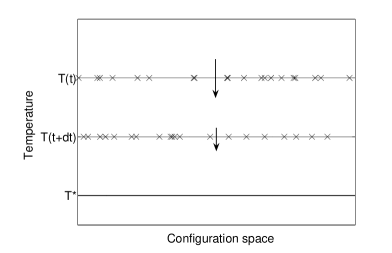
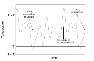
Figure 1: Left: Discretization using several replicas of the system interacting only through the temperature update term. All the replicas are at the same temperature, and estimates of the temperature update term are obtained from the instantaneous distribution of configurations. Right: Single replica discretization. The estimate of the update term at a given temperature is done in analogy with the many replica case, using the previous configurations sampled at the same temperature.

The dynamics (16) is discretized using a splitting procedure, with the decomposition

$$\left\{\begin{array}[]{cl}dq_{t}=&\displaystyle M^{-1}p_{t}\,dt,\\[5.0pt] dp_{t}=&\displaystyle-\nabla V(q_{t})\,dt-\xi M^{-1}p_{t}\,dt+\sqrt{2\xi k_{\rm B}T_{t}}\,dW_{t},\\[5.0pt] dT_{t}=&\displaystyle 0,\\ \end{array}\right.\quad\left\{\begin{array}[]{cl}dq_{t}=&\displaystyle 0,\\[5.0pt] dp_{t}=&\displaystyle 0,\\[5.0pt] dT_{t}=&\displaystyle-\gamma\left(\frac{\displaystyle\int_{0}^{t}A(q_{s},p_{s})\,\delta_{T_{t}-T_{s}}\,ds}{\displaystyle\int_{0}^{t}\delta_{T_{t}-T_{s}}\,ds}\right)\,dt.\\ \end{array}\right.$$

First, the dynamics at a fixed temperature is integrated using some numerical scheme of the general form $(q^{n+1},p^{n+1})=\Phi_{\Delta t,T^{n}}(q^{n},p^{n})$, where $(q^{n},p^{n})$ denotes an approximation of a realization of $(q_{n\Delta t},p_{n\Delta t})$, and the current temperature $T^{n}$ is a parameter of the numerical scheme. For instance, the BBK scheme [6] with the modification of [18] may be used for Langevin dynamics ($i=1,\dots,N$ indexes the particles):

$$\Phi_{\Delta t,T^{n}}\,:\,\left\{\begin{array}[]{c @{= \ } l}p_{i}^{n+1/2}&p_{i}^{n}+\displaystyle\frac{\Delta t}{2}\left(-\nabla_{q_{i}}V(q^{n})-\xi\frac{p_{i}^{n}}{m_{i}}+\frac{1}{2}\sqrt{2\xi\Delta t\,k_{\mathrm{B}}T^{n}}\,G_{i}^{n}\right),\\[10.0pt] q_{i}^{n+1}&\displaystyle q_{i}^{n}+\Delta t\ \frac{p_{i}^{n+1/2}}{m_{i}},\\[10.0pt] p_{i}^{n+1}&\displaystyle\left(1+\frac{\xi\Delta t}{2m_{i}}\right)^{-1}\ \left(p_{i}^{n+1/2}-\frac{\Delta t}{2}\nabla_{q_{i}}V(q^{n+1})+\frac{1}{2}\sqrt{2\xi\Delta t\,k_{\mathrm{B}}T^{n}}\,G_{i}^{n}\right),\\ \end{array}\right.$$

where $\{G_{i}^{n}\}_{i,n}$ are independent standard $3$-dimensional Gaussian random vectors. Of course, there many other implementations of the Langevin dynamics (see for instance [19, 20] and references in [7]). The temperature is then updated after computing the conditional average of the observable $A$ along the trajectory. Finally, the algorithm reads

$$\left\{\begin{array}[]{ccl}(q^{n+1},p^{n+1})&=&\Phi_{\Delta t,T^{n}}(q^{n},p^{n}),\\[5.0pt] T^{n+1}&=&\displaystyle T^{n}-\left(\frac{\displaystyle\sum_{m=0}^{n}A(q^{m},p^{m})\,\chi_{\Delta T}(T^{m}-T^{n})}{\displaystyle\sum_{m=0}^{n}\chi_{\Delta T}(T^{m}-T^{n})}\right)\gamma\Delta t.\\ \end{array}\right.$$ (17)

The ratio in the update term of the temperature is always well-defined provided $\chi_{\Delta T}\geq 0$ and $\chi_{\Delta T}(0)>0$. The functions $\chi_{\Delta T}$ are approximations of Delta functions, and correspond to some binning procedure. For a given temperature, the corresponding bin in the histogram is sought for, and the average value of the observable for this temperature as well as the total number of visits to this bin are updated. More precisely, discretizing the temperature space into regions of width $\Delta T$, a given temperature $T$ can be rewritten as $T=\text{E}(T/\Delta T)\Delta T+R_{T}$, where $\text{E}(x)$ denotes the closest integer to $x$ and $-1/2<R_{T}\leq 1/2$. Then,

$$\chi_{\Delta T}(T^{m}-T^{n})=\left\{\begin{array}[]{cl}1/\Delta T&\text{when }\text{E}(T^{m}/\Delta T)=\text{E}(T^{n}/\Delta T),\\ 0&\text{otherwise}.\end{array}\right.$$

The width $\Delta T$ controls the precision of the final result. It should not be too small, so that the estimates of the (trajectorial) conditional expectations are performed over enough configurations. It may however be refined during the simulation, once close enough to the target temperature.

The choice of parameters, in particular the parameters of the sampling dynamics (such as Nosé-Hoover mass or Langevin friction) and $\gamma$ required for the update of the temperature, is discussed in a specific case in Section 3.2.1.

3.2 A test case: The computation of Hugoniot curves

We present an application of the general sampling algorithm presented in Section 3.1 to the Hugoniot problem described in Section 1.3.1, in the case of noble gases such as Argon. This problem was already studied in [15], where reference results obtained from shock wave simulations are reported.

The interactions within noble gas atoms are well-described by a Lennard-Jones potential:

$$V(q_{1},\dots,q_{N})=\sum_{1\leq i<j\leq N}v(|q_{i}-q_{j}|),\qquad v(r)=4\varepsilon\left(\left(\frac{\sigma}{r}\right)^{12}-\left(\frac{\sigma}{r}\right)^{6}\right).$$

In the case of Argon, $\varepsilon/k_{\rm B}=120$ K and $\sigma=3.405$ Å. It is convenient to use dimensionless parameters to present the results, as is done in [15]. The reduced unit of distance $r_{0}=2^{1/6}\sigma$ corresponds to the minimum of $v$, the unit of mass and energy are respectively the mass of an atom $m$ and $\varepsilon$. Therefore, the unit of time is $\tau=r_{0}\sqrt{m/\varepsilon}$. For Argon, $r_{0}=3.82$ Å, $m=6.64\times 10^{-26}$ kg, $\varepsilon=1.66\times 10^{-21}$ J, and $\tau=2.42\times 10^{-12}$ s. The cut-off used for the computation of the forces is $R_{\rm cut}=2.5\sigma$, and we chose $\Delta T=0.2$ K ($\Delta T=1.67\times 10^{-3}$ in reduced units) for the temperature histograms.

The results presented here are obtained for a crystal reference state, in the cubic face centered geometry, at $T_{0}=10$ K with initial density $\rho_{0}=1.806\times 10^{3}$ kg/m³. The density is chosen so that the initial pressure $P_{0}\simeq 0$.

3.2.1 Choice of parameters

In the case of Hugoniot curves, it is convenient to rewrite the parameter $\gamma$ arising in the update equation for the temperature (16) as

$$\gamma=\frac{\nu}{Nk_{\rm B}},$$

where $\nu>0$ is a frequency. The temperature update can then be recast in a form involving only dimensionless quantities:

$$d\left(\frac{T_{t}}{T_{\text{ref}}}\right)=-\frac{\mathcal{A}_{t}(T_{t})}{Nk_{\rm B}T_{\rm ref}}\,\nu\,dt,\qquad\mathcal{A}_{t}(T)=\frac{\displaystyle\int_{0}^{t}A_{c}(q_{s},p_{s})\,\delta_{T-T_{s}}\,ds}{\displaystyle\int_{0}^{t}\delta_{T-T_{s}}\,ds},$$

since the observable $A_{c}$ (or $A_{xx,c}$), defined by (8) is an extensive quantity homogeneous to an energy. This is then also the case for the average quantity $\mathcal{A}_{t}(T)$. The energy $E_{\text{ref}}=k_{\rm B}T_{\text{ref}}$ is some reference energy per particle. We first discuss the choice of the reference temperature, and then the choice of the frequency $\nu$.

The other parameters have standard values in molecular dynamics simulations: the time step $\Delta t\simeq 0.001$ in reduced units, while the Langevin friction $\xi$ is such that $\xi/m\sim 1/\tau$. Our simulations for Argon were performed with $\Delta t=2\times 10^{-15}$ s^-1 and $\xi/m=10^{12}$ s^-1.

Reference temperature.

The reference temperature is computed from the initial configuration using the estimator of the temperature derived in [15]. Decomposing the microscopic observables associated with the energy and the pressure as

$$H=H_{\text{kin}}+H_{\text{pot}},\qquad P=P_{\text{kin}}+P_{\text{pot}},$$

with

$$H_{\text{kin}}=\frac{1}{2}p^{T}M^{-1}p,\qquad P_{\text{kin}}=\frac{1}{3|\mathcal{D}|}p^{T}M^{-1}p,$$

the Hugoniot problem (9) implies for a given compression $c$:

$$T=\frac{1}{Nk_{\rm B}}\frac{2}{4-c}\left(\langle H\rangle_{|\mathcal{D}|_{0},T_{0}}-\langle V\rangle_{c|\mathcal{D}_{0}|,T}+\frac{1}{2}(\langle P_{\text{pot}}\rangle_{c\mathcal{D}_{0},T}+\langle P\rangle_{|\mathcal{D}|_{0},T_{0}})(1-c)|\mathcal{D}_{0}|\right).$$

Therefore, an estimator of the temperature in terms of the positions $q$ of the particles only is

$$\widehat{T}(q)=\frac{1}{Nk_{\rm B}}\frac{2}{4-c}\left(\langle H\rangle_{|\mathcal{D}_{0}|,T_{0}}-V(q)+\frac{1}{2}(P_{\text{pot}}(q)+\langle P\rangle_{|\mathcal{D}_{0}|,T_{0}})(1-c)|\mathcal{D}_{0}|\right),$$ (18)

which is by construction such that $\displaystyle\left\langle\widehat{T}\right\rangle_{|\mathcal{D}|,T}=T$. The reference temperature is chosen to be

$$T_{\rm ref}=\widehat{T}(q^{0}),$$ (19)

where $q^{0}$ denotes the initial configuration. Usually, this initial configuration is obtained by compressing a perfect lattice in the chosen direction(s). When the compression is not isotropic, the estimator (18) for the initial temperature should be replaced by a similar estimator where the isotropic pressure observable $P$ is replaced by the observable associated with the $P_{xx}$ component of the pressure tensor. The decomposition into kinetic and potential parts of $P_{xx}$ is done as for $P$.

Typical frequency.

Once the reference temperature is set, it is possible to estimate the typical magnitude of the normalized observable

$$\overline{A}_{c}(q,p)=\frac{A_{c}(q,p)}{Nk_{\text{B}}T_{\text{ref}}},$$

for instance by performing some short canonical samplings at fixed compressions and temperatures. The quantity $\overline{A}_{xx,c}$ is defined and estimated in a similar manner. In the case of Hugoniot sampling, Figure 2 presents the distribution of $\overline{A}_{xx,c}$ for canonical samplings performed at different temperatures and anisotropic compressions. The typical values of $\overline{A}_{xx,c}$ are of order $\triangle\overline{A}_{xx,c}\sim 0.5$. This gives a typical size for the term appearing in the equation on the temperature since the temperature is updated by a factor of order $\triangle\overline{A}_{xx,c}\nu\Delta t$ at each time step. The magnitude of $\nu$ should be chosen such that the evolution of the temperature is not too fast (as suggested by Theorems 2 and 3). For instance,

$$\frac{\delta T}{T_{\text{ref}}}=\triangle\overline{A}_{xx,c}\nu\Delta t\sim 10^{-3}-10^{-1}.$$ (20)

Typical time integration steps are $\Delta t=10^{-3}-10^{-2}$ in reduced units. The parameter $\nu$ can then be found from the above heuristic rule.

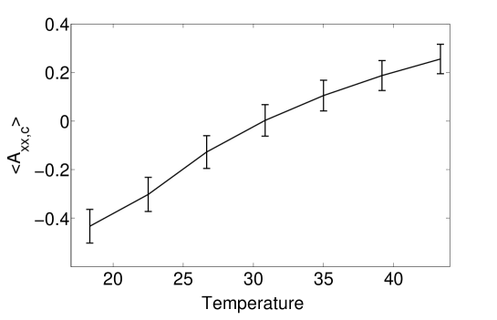
Figure 2: Distribution of $\overline{A}_{xx,c}$ (in reduced units) for an anisotropic compression $c=0.62$ as a function of temperature. The error bars are equal to twice the standard deviation of $\overline{A}_{xx,c}$ obtained for a system of $N=4,000$ atoms, and are meant to give an order of magnitude of the width of the distribution of values of $\overline{A}_{xx,c}$.

In the Hugoniot example, the rule (20) gives an estimate of possible values of the frequency. For Argon at a compression $c=0.62$, $\nu=10^{15}$ s^-1 seems a reasonable choice. The results of Figures 3 and 4, obtained for systems of $N=4,000$ and $N=32,000$ atoms respectively, show that the temperature converges with the method presented here, and that frequencies around $\nu=10^{15}$ s^-1 are indeed a reasonable choice. For smaller frequencies, the convergence is slower, whereas larger frequencies trigger fast initial oscillations which may lead to numerical instabilities in the scheme. In any case however, the final result does not depend on the value of $\nu$, which shows the robustness of the method. It may be interesting to increase the value of $\nu$ as the typical values of the observable decrease during the simulation (see also Remark 1).

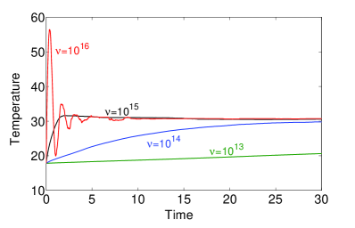
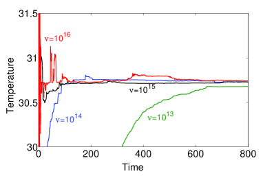
Figure 3: (color online) Plot of the temperature as a function of time (in reduced units) for different values of the frequency $\nu$ (in $s^{-1}$), for a system of size $N=4,000$.

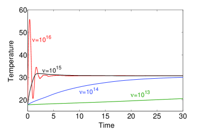
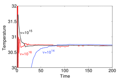
Figure 4: (color online) Plot of the temperature as a function of time (in reduced units) for different values of the frequency $\nu$ (in $s^{-1}$), for a system of size $N=32,000$.

3.2.2 Hugoniot curve

We present in Figure 5 the Hugoniot curve obtained for a system of $N=4,000$ particles, using the parameters given in Section 3.2.1, with $\nu=10^{14}$ s^-1 for compressions $c\leq 0.7$ (temperatures around 4 and less, in reduced units) and $\nu=10^{15}$ s^-1 for higher compressions. This curve is obtained by considering many different anisotropic compressions, and computing the temperature as well as the associated average pressure $P$ in the system. The results are in very good agreement with [15], which validates the method.

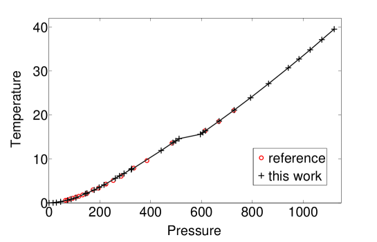
Figure 5: (color online) Hugoniot curve for Argon (in reduced units), computed using the method presented in this work (black solid line and crosses). The reference results from [15] are also reported (red circles).

4 Proofs of the mathematical results

4.1 Proof of Theorem 1

Existence of a time $\tau>0$ where the temperature remains positive.

Assume that $\psi(t,\cdot)\in\mathrm{L}^{1}(\mathcal{M})$ and $\psi\geq 0$, so that $\|\psi(t,\cdot)\|_{\mathrm{L}^{1}}=1$. Then, since the temperature derivative is bounded by $\gamma\|A\|_{\infty}$, there exists a time $\tau>0$ such that $|T(t)-T^{0}|\leq T^{0}/2$ for all $t\in[0,\tau]$. For instance,

$$\tau=\frac{T^{0}}{2\gamma\|A\|_{\infty}}>0,$$ (21)

where $\|A\|_{\infty}=\sup\,\{\,|A(q)|,\ q\in\mathcal{M}\,\}$. This choice ensures that the temperature remains positive. We will show below that $\psi\in\mathrm{L}^{1}(\mathcal{M})$ since $\psi\in\mathrm{L}^{2}(\mathcal{M})$ and $|\mathcal{M}|<+\infty$.

Construction of a solution through a fixed point application.

We show the existence of a solution using a fixed-point theorem. Denote

$$E=\mathrm{C}^{1}([0,\tau],\mathbb{R})\cap\left\{\frac{T^{0}}{2}\leq T\leq\frac{3T^{0}}{2}\right\}\cap\{T(0)=T^{0}\}\cap\{|T^{\prime}|\leq\gamma\|A\|_{\infty}\}.$$

This set is a bounded closed convex subset of $\mathrm{C}^{1}([0,\tau],\mathbb{R})$. Consider the mapping

$$g\ :\ \begin{array}[]{ccccccc}E&\longrightarrow&\mathrm{C}^{0}([0,\tau],\mathrm{H}^{2}(\mathcal{M}))&\longrightarrow&\mathrm{C}^{2}([0,\tau],\mathbb{R})\cap E&\longrightarrow&E\\ T&\longmapsto&\psi_{T}&\longmapsto&g(T)&\longmapsto&g(T)\\ \end{array}$$ (22)

The construction of $\psi_{T}$ from a given temperature function $T$ is performed using the equation

$$\partial_{t}\psi_{T}=k_{\rm B}T(t)\,\nabla\cdot\left[\mu_{T(t)}\nabla\left(\frac{\psi_{T}}{\mu_{T(t)}}\right)\right]=k_{\rm B}T(t)\Delta\psi_{T}+\nabla V\cdot\nabla\psi_{T}+\Delta V\psi_{T},$$ (23)

and the temperature function $g(T)$ is then recovered using the second equation in (15), namely

$$g(T)(t)=T^{0}-\gamma\int_{0}^{t}\int_{\mathcal{M}}A(q)\,\psi_{T}(s,q)\,dq\,ds.$$

Regularity of $\psi_{T}$ given $T$.

The equation (23) is of the general type

$$\partial_{t}\psi_{T}+\mathcal{L}_{T}(t)\psi_{T}=0,$$ (24)

where the family of operators $\{\mathcal{L}_{T}(t)\}_{t\geq 0}$ have constant domains $D=\mathrm{H}^{2}(\mathcal{M})$, and

$$\mathcal{L}_{T}(t)\psi=-k_{\rm B}T(t)\,\nabla\cdot\left[\mu_{T(t)}\nabla\left(\frac{\psi}{\mu_{T(t)}}\right)\right]=-\nabla\cdot\left(k_{\rm B}T(t)\,\nabla\psi+\nabla V\psi\right).$$

It is enough to show the regularity of the solution of $\partial_{t}\widetilde{\psi}+(\eta+\mathcal{L}_{T}(t))\widetilde{\psi}=0$ since the latter equation is related to the original equation (24) through the transform $\psi_{T}=\exp(\eta t)\widetilde{\psi}$.

For a fixed $t$ and $f\in\mathrm{L}^{2}(\mathcal{M})$, consider the equation

$$(\eta+\mathcal{L}_{T}(t))u=f.$$ (25)

Lax-Milgram’s theorem shows that there is a unique solution $u\in\mathrm{H}^{1}(\mathcal{M})$. Indeed, $(u,v)\mapsto\langle u,(\eta+\mathcal{L}_{T}(t))v\rangle$ can be extended to a functional on $\mathrm{H}^{1}(\mathcal{M})^{2}$ using

$$\left|\langle u,(\eta+\mathcal{L}_{T}(t))v\rangle\right|=\left|\int_{\mathcal{M}}\eta uv+k_{\rm B}T(t)\nabla u\cdot\nabla v+v\nabla u\cdot\nabla V\right|\\ \leq C\|u\|_{\mathrm{H}^{1}}\,\|v\|_{\mathrm{H}^{1}},\\$$

where the constant $C$ depends only on $\|\nabla V\|_{\infty}$ and on $T^{0}$ (actually on the upper bound of the temperature). Besides, $u\in D\mapsto\langle u,(\eta+\mathcal{L}_{T}(t))u\rangle$, extended to a quadratic form on $\mathrm{H}^{1}(\mathcal{M})$, is coercive on this space for $\eta$ large enough since

$$\langle u,(\eta+\mathcal{L}_{T}(t))u\rangle = \int_{\mathcal{M}}\eta\,u^{2}+k_{\rm B}T(t)|\nabla u|^{2}+u\nabla u\cdot\nabla V$$

$$\geq \frac{k_{\rm B}T^{0}}{2}\int_{\mathcal{M}}|\nabla u|^{2}+\eta\int_{\mathcal{M}}u^{2}-\frac{1}{2}\|\nabla V\|_{\infty}\left(\alpha\int_{\mathcal{M}}|\nabla u|^{2}+\frac{1}{\alpha}\int_{\mathcal{M}}u^{2}\right)$$

$$\geq c\|u\|_{\mathrm{H}^{1}}^{2},$$

for $\eta$ large enough (choosing first $\alpha<k_{\rm B}T^{0}/\|\nabla V\|_{\infty}$ and then $\eta>\|\nabla V\|_{\infty}/2\alpha$). Again, the constant $c$ depends only on $\|\nabla V\|_{\infty}$ and on $T^{0}$. The solution $u$ of (25) is in fact such that

$$\Delta u=\frac{1}{k_{\rm B}T(t)}\left(\eta u-\nabla V\cdot\nabla u-u\Delta V-f\right)\in\mathrm{L}^{2}(\mathcal{M}),$$

so that $u\in D$. It is easily seen that the mapping $f\mapsto u=(\lambda+\eta+\mathcal{L}_{T}(t))^{-1}f$ for $\lambda\in\mathbb{C}$ with $\mathrm{Re}(\lambda)\geq 0$ is continous, and bounded by $M/(1+|\lambda|)$ for some $M>0$.

Besides, for $0\leq r,s,t\leq\tau$,

$$\|\left[(\eta+\mathcal{L}_{T}(r))-(\eta+\mathcal{L}_{T}(s))\right](\eta+\mathcal{L}_{T}(t))^{-1}\|_{\mathcal{L}(\mathrm{L}^{2},\mathrm{L}^{2})} = k_{\rm B}|T(r)-T(s)|\|\Delta(\eta+\mathcal{L}_{T}(t))^{-1}\|_{\mathcal{L}(\mathrm{L}^{2},\mathrm{L}^{2})}$$

$$\leq c|T(r)-T(s)|\leq C|r-s|,$$

for some constants $C,c>0$ since $T$ is $\mathrm{C}^{1}$.

The results of Kato [14] then show the existence of a unique solution $\psi_{T}\in\mathrm{C}^{0}([0,\tau],\mathrm{H}^{2}(\mathcal{M}))$ and hence $\psi_{T}\in\mathrm{C}^{0}([0,\tau],\mathrm{H}^{1}(\mathcal{M}))$. Bounds on the $\mathrm{H}^{1}(\mathcal{M})$ norm of $\psi_{T}$ in terms of the bounds on $T$ are obtained with a Gronwall inequality:

$$\partial_{t}\left(\frac{1}{2}\|\psi_{T}\|^{2}_{\mathrm{H}^{1}}\right) = \int_{\mathcal{M}}(\psi_{T}-\Delta\psi_{T})\nabla\left(k_{\rm B}T(t)\nabla\psi_{T}+\nabla V\psi_{T}\right)$$

$$= -k_{\rm B}T(t)\int_{\mathcal{M}}|\nabla\psi_{T}|^{2}+|\Delta\psi_{T}|^{2}-\int_{\mathcal{M}}\Delta\psi_{T}\nabla V\cdot\nabla\psi_{T}$$

$$\quad+\int_{\mathcal{M}}|\psi_{T}|^{2}\Delta V+\psi_{T}\nabla V\cdot\nabla\psi_{T}-\int_{\mathcal{M}}\psi_{T}\Delta\psi_{T}\Delta V.$$

Using the following Cauchy-Schwarz inequalities to bound the terms involving $\Delta\psi_{T}$:

$$\left|\int_{\mathcal{M}}\Delta\psi_{T}\nabla V\cdot\nabla\psi_{T}\right|\leq\frac{k_{\rm B}T^{0}}{4}\int_{\mathcal{M}}|\Delta\psi_{T}|^{2}+\frac{\|\nabla V\|^{2}_{\infty}}{k_{\rm B}T^{0}}\int_{\mathcal{M}}|\nabla\psi_{T}|^{2},$$

$$\left|\int_{\mathcal{M}}\psi_{T}\Delta\psi_{T}\Delta V\right|\leq\frac{k_{\rm B}T^{0}}{4}\int_{\mathcal{M}}|\Delta\psi_{T}|^{2}+\frac{\|\Delta V\|^{2}_{\infty}}{k_{\rm B}T^{0}}\int_{\mathcal{M}}|\psi_{T}|^{2},$$

it follows

$$\partial_{t}\left(\frac{1}{2}\|\psi_{T}\|^{2}_{\mathrm{H}^{1}}\right) \leq -k_{\rm B}T(t)\int_{\mathcal{M}}|\nabla\psi_{T}|^{2}+\int_{\mathcal{M}}|\psi_{T}|^{2}\Delta V+\psi_{T}\nabla V\cdot\nabla\psi_{T}+\frac{\|\nabla V\|^{2}_{\infty}+\|\Delta V\|^{2}_{\infty}}{k_{\rm B}T^{0}}\|\psi_{T}\|^{2}_{\mathrm{H}^{1}}$$

$$\leq K\|\psi_{T}\|^{2}_{\mathrm{H}^{1}},$$

where the constant $K>0$ depends only on $V$ and its derivatives, and on $T^{0}$ (actually, the lower bound of the temperature). This shows that

$$\|\psi_{T}(t,\cdot)\|_{\mathrm{H}^{1}}\leq\exp(\tau K)\|\psi^{0}\|_{\mathrm{H}^{1}}$$

for all $0\leq t\leq\tau$.

Regularity of $g(T)$ given $\psi$.

From the equation on the temperature:

$$g(T)^{\prime}(t)=-\gamma\int_{\mathcal{M}}A(q)\,\psi_{T}(t,q)\,dq,$$

it follows

$$g(T)^{\prime\prime}(t)=\gamma\int_{\mathcal{M}}(\nabla A\cdot\nabla V-k_{\rm B}T(t)\Delta A)\psi_{T},$$

and

$$g(T)^{(3)}(t)=-\gamma\int_{\mathcal{M}}\nabla\cdot(\nabla A\cdot\nabla V-k_{\rm B}T(t)\Delta A)(\nabla V\psi_{T}+k_{\rm B}T(t)\nabla\psi_{T})-\gamma k_{\rm B}T^{\prime}(t)\int_{\mathcal{M}}\Delta A\psi_{T}.$$

Therefore, $|g(T)^{(3)}(t)|\leq\gamma C_{A,V}\|T\|_{\mathrm{C}^{1}}(1+\|T\|_{\mathrm{C}^{1}})\,\|\psi_{T}(t,\cdot)\|_{\mathrm{H}^{1}}$, where $C_{A,V}$ depends only on $\|\mathcal{M}|$ and on $\mathrm{L}^{\infty}$ bounds on $A,V$ and their derivatives (up to the order 3 for $A$, and to the order 2 for $V$). Uniform bounds on $g(T)^{\prime\prime}$ are recovered by time integration:

$$\sup_{0\leq t\leq\tau}|g(T)^{\prime\prime}(t)| \leq |g(T)^{\prime\prime}(0)|+\tau\|g(T)^{(3)}\|_{\infty}$$

$$\leq \gamma\left(\widetilde{C}_{A,V}\|\psi^{0}\|_{\mathrm{H}^{1}}+\tau C_{A,V}\|T\|_{\mathrm{C}^{1}}\,(1+\|T\|_{\mathrm{C}^{1}})\|\psi\|_{\mathrm{C}^{0}([0,T],\mathrm{H}^{1})}\right)$$

$$\leq \gamma\left[\widetilde{C}_{A,V}+\tau C_{A,V}\|T\|_{\mathrm{C}^{1}}(1+\|T\|_{\mathrm{C}^{1}})\,\exp(K\tau)\right]\|\psi^{0}\|_{\mathrm{H}^{1}}\leq M,$$

for some $M>0$ (depending on $\tau$, $\psi^{0}$, $T^{0}$). Since $\|g(T)^{\prime}\|_{\infty}\leq\gamma\|A\|_{\infty}$, bounds on $g(T),g(T)^{\prime}$ consistent with the set $E$ are still valid with the choice of $\tau$ given by (21). This shows finally that $g(T)$ belongs to a bounded set of $\mathrm{C}^{2}([0,\tau],\mathbb{R})$.

Existence of a fixed point.

The mapping $g$ is continuous from the bounded closed convex set $E$ to istself, and in fact compact since the injection $\mathrm{C}^{2}([0,\tau],\mathbb{R})\cap\{|T^{\prime\prime}|\leq M\}\cap E\hookrightarrow E$ is compact. Schauder’s theorem (see for instance [21]) shows that there exists $T\in E$ such that $g(T)=T$, therefore giving the existence of a solution to the equation (15).

Uniqueness.

Consider two solutions $(T_{1},\psi_{1})$ and $(T_{2},\psi_{2})$ starting from the same initial condition $(T^{0},\psi^{0})$. Then, on the interval $[0,\tau]$,

$$\frac{d}{dt}\left(\frac{1}{2}(T_{1}(t)-T_{2}(t))^{2}\right) = -\gamma(T_{1}(t)-T_{2}(t))\int_{\mathcal{M}}A\,(\psi_{1}-\psi_{2})$$

$$\leq \sqrt{|\mathcal{M}|}\|A\|_{\infty}\,|T_{1}(t)-T_{2}(t)|\,\|\psi_{1}-\psi_{2}\|_{\mathrm{L}^{2}}.$$

Moreover,

$$\frac{d}{dt}\left(\frac{1}{2}\|\psi_{1}-\psi_{2}\|_{\mathrm{L}^{2}}^{2}\right) = -\int_{\mathcal{M}}\nabla V\cdot\nabla(\psi_{1}-\psi_{2})(\psi_{1}-\psi_{2})-k_{\rm B}\frac{T_{1}(t)+T_{2}(t)}{2}\int_{\mathcal{M}}|\nabla(\psi_{1}-\psi_{2})|^{2}$$

$$\quad-k_{\rm B}\frac{T_{1}(t)-T_{2}(t)}{2}\int_{\mathcal{M}}\nabla(\psi_{1}+\psi_{2})\cdot\nabla(\psi_{1}-\psi_{2})$$

$$\leq \quad c_{1}\|\psi_{1}-\psi_{2}\|_{\mathrm{L}^{2}}^{2}+c_{2}|T_{1}(t)-T_{2}(t)|^{2}\int_{\mathcal{M}}|\nabla(\psi_{1}+\psi_{2})|^{2},$$

for some constants $c_{1},c_{2}>0$. Indeed, the the $\nabla(\psi_{1}-\psi_{2})$ contributions of the first and third terms on the right hand side of the first line can be cancelled using the inequality $2ab\leq a^{2}/\eta+\eta b^{2}$ and

$$-k_{\rm B}\frac{T_{1}(t)+T_{2}(t)}{2}\int_{\mathcal{M}}|\nabla(\psi_{1}-\psi_{2})|^{2}\leq-\frac{k_{\rm B}T^{0}}{2}\int_{\mathcal{M}}|\nabla(\psi_{1}-\psi_{2})|^{2}.$$

In view of the uniform bounds on $\|\nabla\psi_{1}(t,\cdot)\|_{\mathrm{L}^{2}}$, $\|\nabla\psi_{2}(t,\cdot)\|_{\mathrm{L}^{2}}$,

$$\frac{d}{dt}\left(\frac{1}{2}(T_{1}(t)-T_{2}(t))^{2}+\frac{1}{2}\|\psi_{1}-\psi_{2}\|_{\mathrm{L}^{2}}^{2}\right)\leq C\left(\frac{1}{2}(T_{1}(t)-T_{2}(t))^{2}+\frac{1}{2}\|\psi_{1}-\psi_{2}\|_{\mathrm{L}^{2}}^{2}\right)$$

for some $C>0$. As

$$\frac{1}{2}(T_{1}(0)-T_{2}(0))^{2}+\frac{1}{2}\|\psi_{1}(0,\cdot)-\psi_{2}(0,\cdot)\|_{\mathrm{L}^{2}}^{2}=0,$$

a Gronwall inequality shows that $T_{1}=T_{2}$ and $\psi_{1}=\psi_{2}$ for all $0\leq t\leq\tau$.

Positivity of $\psi$ for relative entropy estimates.

It is important that $\psi>0$ for the Fisher information to be defined in the case of relative entropy estimates (see the proof of Theorem 2 in Section 4.2). In any cases, the density $\psi$ has to remain non-negative.

Consider

$$\Phi(t,q)=\psi(s(t),q),$$ (26)

where the function $t\mapsto s(t)$ is defined through the ordinary differential equation:

$$s^{\prime}(t)=\frac{1}{k_{\rm B}T(s(t))}.$$

The function $s$ is well defined (since $T>0$), continuous and in fact $\mathrm{C}^{1}$, and strictly increasing hence invertible. The evolution of the density $\Phi$ is obtained by solving

$$\partial_{t}\Phi=\Delta\Phi+\frac{1}{k_{\rm B}T(s(t))}\nabla\cdot(\Phi\nabla V)=\Delta\Phi+\frac{1}{k_{\rm B}\widetilde{T}(t)}\nabla\cdot(\Phi\nabla V),$$ (27)

with $\widetilde{T}(t)=T(s(t))$. The density $\psi$ is recovered with (26) since $s$ is invertible. The function $\phi=\Phi/\sqrt{\mu_{\widetilde{T}(t)}}$ satisfies

$$\partial_{t}\phi(t,x)=\Delta\phi(t,x)+W(t,x)\phi(x),$$

where the potential

$$W(t,x)=\frac{1}{2k_{\rm B}\widetilde{T}(t)}\left(\Delta V(x)-\frac{1}{2k_{\rm B}\widetilde{T}(t)}|\nabla V(x)|^{2}-\frac{\widetilde{T}^{\prime}(t)}{\widetilde{T}(t)}V(x)\right)$$

is bounded. Since $\mu_{T}$ is positive and uniformly bounded from below, it is enough to show that $\phi(t,\cdot)>0$ to have $\psi(t,\cdot)>0$. The function $\widetilde{\phi}=\exp(t\|W\|_{\infty})\phi$ satisfies

$$(\partial_{t}-\Delta)\widetilde{\phi}=(W(t,x)+\|W\|_{\infty})\widetilde{\phi}\geq 0.$$

Therefore, $\widetilde{\phi}(t,\cdot)\geq\inf\widetilde{\phi}(0,\cdot)$, and so, $\phi(t,x)\geq m\exp(-t\|W\|_{\infty})>0$ provided $\phi(0,\cdot)\geq m>0$. This shows that $\psi>0$ provided $\psi^{0}>0$. Similarly, $\psi\geq 0$ provided $\psi^{0}\geq 0$.

4.2 Proof of Theorem 2

General strategy of the proof.

We first consider the solution of (15) on a time interval $[0,\tau]$ as given by Theorem 1, possibly reducing $\tau$ so that $T(t)\in I_{T}^{A}\cap T_{T}^{\mathrm{LSI}}$ for all $0\leq t\leq\tau$. We then show (see below) that this implies $\mathcal{E}^{\prime}(t)\leq-\kappa\mathcal{E}(t)$ for some some $\kappa>0$. This will show that $\mathcal{E}$ decreases, and so $T$ remains in $I_{T}^{A}\cap T_{T}^{\mathrm{LSI}}$ since $|T(t)-T^{\ast}|\leq\sqrt{2\mathcal{E}(t)}\leq\sqrt{2\mathcal{E}(0)}\leq\sqrt{2\mathcal{E}^{*}}$. The solution can then be continued at all times $t\geq 0$ using repeatedly the arguments of the proof of Theorem 1, upon replacing the set $E$ in the definition of $g$ given in (22) by the closed convex bounded set $E=\mathrm{C}^{1}([n\tau,(n+1)\tau],\mathbb{R})\cap\{T\in I_{T}^{A}\cap T_{T}^{\mathrm{LSI}}\}\cap\{T(n\tau)=T^{n\tau}\}\cap\{|T^{\prime}|\leq\gamma\|A\|_{\infty}\}$, where $T^{n\tau}$ is the final value of the solution on the interval $[(n-1)\tau,n\tau]$ (for $n\geq 1$). The main difference with the proof of Section 4.1 is that uniform (upper and lower) bounds on the temperature are provided thanks to the decrease of the entropy.

Proof of the Gronwall inequality $\mathcal{E}^{\prime}(t)\leq-\kappa\mathcal{E}(t)$.

With the function $h$ chosen here,

$$\frac{dE(t)}{dt} = -k_{\rm B}T(t)\,\int_{\mathcal{M}}\frac{|\nabla f|^{2}}{f}\,\mu_{T(t)}-\frac{T^{\prime}(t)}{k_{\mathrm{B}}T(t)^{2}}\int_{\mathcal{M}}(f-1)\,\left(V-\left\langle V\right\rangle_{T(t)}\right)\,\mu_{T(t)}$$

$$\leq -\rho k_{\rm B}T(t)\,E(t)+\frac{2|T^{\prime}(t)|\,\|V\|_{\infty}}{k_{\mathrm{B}}T(t)^{2}}\int_{\mathcal{M}}|f-1|\,\mu_{T(t)}$$

$$\leq -\rho k_{\rm B}T(t)\,E(t)+\frac{4|T^{\prime}(t)|\,\|V\|_{\infty}}{k_{\mathrm{B}}T(t)^{2}}\sqrt{E(t)},$$

where we have used the Csizár-Kullback inequality

$$\int_{\mathcal{M}}|f-1|\,\mu_{T(t)}\leq 2\sqrt{E(t)}$$

in the last step. The derivative of the temperature can be bounded using

$$T^{\prime}(t)=-\gamma\int_{\mathcal{M}}A\psi_{t}=-\gamma\left(\left\langle A\right\rangle_{T(t)}+\int_{\mathcal{M}}A(f-1)\mu_{T(t)}\right),$$

which shows that

$$|T^{\prime}(t)| \leq \gamma\left(\left|\left\langle A\right\rangle_{T(t)}-\left\langle A\right\rangle_{T^{\ast}}\right|+\left|\int_{\mathcal{M}}A\psi_{t}-\int_{\mathcal{M}}A\mu_{T(t)}\right|\right)$$

$$\leq \gamma\left(a\left|T(t)-T^{\ast}\right|+\left|\int_{\mathcal{M}}A\psi_{t}-\int_{\mathcal{M}}A\mu_{T(t)}\right|\right)$$

$$\leq \gamma\left(a\left|T(t)-T^{\ast}\right|+2\|A\|_{\infty}\sqrt{E(t)}\right),$$

using Assumption 2 and the Csizár-Kullback inequality to bound the second term on the right-hand side. These estimates are also helpful for bounding the derivative of the temperature entropy:

$$\frac{d}{dt}\left[\frac{1}{2}(T(t)-T^{\ast})^{2}\right] = -\gamma\left(\left\langle A\right\rangle_{T(t)}+\int_{\mathcal{M}}A(f-1)\mu_{T(t)}\right)(T(t)-T^{\ast})$$

$$\leq -\gamma\left(\left\langle A\right\rangle_{T(t)}-\left\langle A\right\rangle_{T^{\ast}}\right)(T(t)-T^{\ast})+2\gamma\|A\|_{\infty}\left|T(t)-T^{\ast}\right|\sqrt{E(t)}$$

$$\leq -\alpha\gamma(T(t)-T^{\ast})^{2}+2\gamma\|A\|_{\infty}\left|T(t)-T^{\ast}\right|\sqrt{E(t)},$$

where Assumption 2 has been used again. Gathering the estimates,

$$\frac{d\mathcal{E}(t)}{dt} \leq -\rho k_{\rm B}T(t)\,E(t)+\frac{4\gamma\,\|V\|_{\infty}}{k_{\mathrm{B}}T(t)^{2}}\sqrt{E(t)}\left(a\left|T(t)-T^{\ast}\right|+2\|A\|_{\infty}\sqrt{E(t)}\right)$$

$$-\alpha\gamma(T(t)-T^{\ast})^{2}+2\gamma\|A\|_{\infty}\left|T(t)-T^{\ast}\right|\sqrt{E(t)}$$

$$\leq -\left(\rho k_{\rm B}T(t)-\frac{8\gamma\,\|V\|_{\infty}\|A\|_{\infty}}{k_{\mathrm{B}}T(t)^{2}}\right)E(t)-\alpha\gamma(T(t)-T^{\ast})^{2}$$

$$+\gamma\left(2\|A\|_{\infty}+\frac{4a\,\|V\|_{\infty}}{k_{\mathrm{B}}T(t)^{2}}\right)\sqrt{E(t)}\left|T(t)-T^{\ast}\right|$$

$$\leq -\left[\rho k_{\rm B}T(t)-\frac{8\gamma\,\|V\|_{\infty}\|A\|_{\infty}}{k_{\mathrm{B}}T(t)^{2}}-\frac{\gamma}{\eta}\left(\|A\|_{\infty}+\frac{2a\,\|V\|_{\infty}}{k_{\mathrm{B}}T(t)^{2}}\right)\right]E(t)$$

$$-\gamma\left[\alpha-\eta\left(\|A\|_{\infty}+\frac{2a\,\|V\|_{\infty}}{k_{\mathrm{B}}T(t)^{2}}\right)\right](T(t)-T^{\ast})^{2},$$

where the inequality $\displaystyle ab\leq\frac{1}{2\eta}a^{2}+\frac{\eta}{2}b^{2}$ (for any $\eta>0$) has been used in the last step. This estimate shows that, with $\eta=\sqrt{\gamma}$ for instance, and choosing $\gamma$ small enough such that

$$\rho k_{\rm B}\min(T^{A}_{\mathrm{min}},T^{\mathrm{LSI}}_{\mathrm{min}})-\frac{8\gamma\,\|V\|_{\infty}\|A\|_{\infty}}{k_{\mathrm{B}}\min(T^{A}_{\mathrm{min}},T^{\mathrm{LSI}}_{\mathrm{min}})^{2}}-\sqrt{\gamma}\left(\|A\|_{\infty}+\frac{2a\,\|V\|_{\infty}}{k_{\mathrm{B}}\min(T^{A}_{\mathrm{min}},T^{\mathrm{LSI}}_{\mathrm{min}})^{2}}\right)>0,$$

$$\alpha-\sqrt{\gamma}\left(\|A\|_{\infty}+\frac{2a\,\|V\|_{\infty}}{k_{\mathrm{B}}\min(T^{A}_{\mathrm{min}},T^{\mathrm{LSI}}_{\mathrm{min}})^{2}}\right)>0,$$

there exists $\kappa>0$ such that

$$\frac{d\mathcal{E}(t)}{dt}\leq-\kappa\mathcal{E}(t).$$

Therefore, the entropy decreases, and the initial bounds on the temperature are satisfied at all times. Gronwall’s lemma finally shows that $\mathcal{E}(t)\to 0$ exponentially fast.

Remark 3 (Nonlinear feedback).

Convergence results for a nonlinear temperature feedback of the form (14) for a nonlinear function $f$ such that $f(x)=0$ if and only if $x=0$, can be proved by extending the proofs of this section to the case when

$$\forall R>0,\quad\exists c_{1},c_{2}>0\ \ \textrm{such that}\ \ \forall x\in[-R,R],\quad c_{1}\leq\frac{f(x)}{x}\leq c_{2}.$$ (28)

The constant $R$ is related to the maximal value of $\displaystyle\int_{\mathcal{M}}A\psi_{t}$, which is dictated by the initial entropy $\mathcal{E}(0)$: if $\mathcal{E}(t)\leq\mathcal{E}(0)$, then the temperature $T(t)$ belongs to a bounded set $I_{\mathcal{E}(0)}$, and so, for usual entropy functions,

$$\left|\int_{\mathcal{M}}A(q)\psi_{t}(q)\,dq\right|\leq|\langle A\rangle_{T(t)}|+\int_{\mathcal{M}}A|f-1|\mu_{T(t)}\,dq\leq\sup_{T\in I_{\mathcal{E}(0)}}|\langle A\rangle_{T}|+c\sqrt{\mathcal{E}(t)}\leq R,$$

where $R$ depends only on $\mathcal{E}(0)$, and $c$ depends on the choice of the entropy function ($c=2$ for relative entropies). This shows why the bounds (28) on some compact interval only are sufficient. For the choice $f(x)=x+x^{3}$ for instance, $c_{1}=1$ and $c_{2}=1+R^{2}$. Such choices may be helpful in numerical simulations to accelerate the convergence toward the temperature of interest at the early stages of the process.

4.3 Proof of Theorem 3

The proof follows the same lines as the proof of Theorem 2, and we present only the modifications required in the case considered here. The first change in the proof is in the bound of the derivative of the spatial entropy $E(t)$. It holds

$$\frac{dE(t)}{dt} = -k_{\rm B}T(t)\int_{\mathcal{M}}\left|\nabla f\right|^{2}\,\mu_{T(t)}+\frac{T^{\prime}(t)}{k_{\mathrm{B}}T(t)^{2}}\int_{\mathcal{M}}\left[h(f)-(f-1)\,f\right]\,\left(V-\left\langle V\right\rangle_{T(t)}\right)\,\mu_{T(t)}$$

$$= -\rho k_{\rm B}T(t)\,E(t)-\frac{T^{\prime}(t)}{k_{\mathrm{B}}T(t)^{2}}\int_{\mathcal{M}}\left[h(f)+f-1\right]\,\left(V-\left\langle V\right\rangle_{T(t)}\right)\,\mu_{T(t)}$$

$$\leq -\left(\rho k_{\rm B}T(t)-\frac{2|T^{\prime}(t)|\,\|V\|_{\infty}}{k_{\mathrm{B}}T(t)^{2}}\right)E(t)+\frac{2|T^{\prime}(t)|\|V\|_{\infty}}{k_{\mathrm{B}}T(t)^{2}}\int_{\mathcal{M}}|f-1|\,\mu_{T(t)}$$

$$\leq -\left(\rho k_{\rm B}T(t)-\frac{2|T^{\prime}(t)|\,\|V\|_{\infty}}{k_{\mathrm{B}}T(t)^{2}}\right)E(t)+\frac{2\sqrt{2}|T^{\prime}(t)|\|V\|_{\infty}}{k_{\mathrm{B}}T(t)^{2}}\sqrt{E(t)}$$

where we have used the Cauchy-Schwarz inequality

$$\int_{\mathcal{M}}|f-1|\,\mu_{T(t)}\leq\sqrt{\int_{\mathcal{M}}|f-1|^{2}\,\mu_{T(t)}}\sqrt{\int_{\mathcal{M}}\mu_{T(t)}}=\sqrt{2E(t)}.$$

A Cauchy-Schwarz inequality is also used to establish a slighty different bound on the temperature derivative:

$$|T^{\prime}(t)|\leq\gamma\left(a\left|T(t)-T^{\ast}\right|+\|A\|_{\infty}\sqrt{2E(t)}\right),$$

and

$$\frac{d}{dt}\left[\frac{1}{2}(T(t)-T^{\ast})^{2}\right]\leq-\alpha\gamma(T(t)-T^{\ast})^{2}+\gamma\|A\|_{\infty}\left|T(t)-T^{\ast}\right|\sqrt{2E(t)}.$$

The spatial entropy derivative can then be bounded as

$$\frac{dE(t)}{dt}\leq-\left[\rho k_{\rm B}T(t)-\gamma\frac{4\|A\|_{\infty}\,\|V\|_{\infty}}{k_{\mathrm{B}}T(t)^{2}}\left(1+\sqrt{\frac{E(t)}{2}}\right)\right]E(t)+\frac{2a\gamma\|V\|_{\infty}}{k_{\mathrm{B}}T(t)^{2}}|T(t)-T^{\ast}|\left(E(t)+\sqrt{2E(t)}\right).$$

For the total entropy,

$$\frac{d\mathcal{E}(t)}{dt} \leq -\left[\rho k_{\rm B}T(t)-\gamma\frac{4\|A\|_{\infty}\,\|V\|_{\infty}}{k_{\mathrm{B}}T(t)^{2}}\left(1+\sqrt{\frac{E(t)}{2}}\right)\right]E(t)-\alpha\gamma(T(t)-T^{\ast})^{2}$$

$$+\sqrt{2}\gamma\left[\frac{2a\|V\|_{\infty}}{k_{\mathrm{B}}T(t)^{2}}\left(1+\sqrt{\frac{E(t)}{2}}\right)+\|A\|_{\infty}\right]|T(t)-T^{\ast}|\sqrt{E(t)}.$$

This estimate is analogous to the one obtained in the relative entropy case, except for some additional factors $\sqrt{E(t)}$, which are bounded by $\sqrt{\mathcal{E}(t)}$, hence by $\sqrt{\mathcal{E}(0)}$ when the total entropy decreases. However, it is easily seen that, taking initial conditions $\mathcal{E}(0)\leq\mathcal{E}^{\ast}$and for $\gamma$ small enough, the function $\mathcal{E}$ is decreasing and bounded by $\mathcal{E}(0)$. There exists then $\kappa>0$ such that $\mathcal{E}^{\prime}(t)\leq-\kappa\mathcal{E}(t)$, which again implies the longtime convergence.

Acknowledgements

We thank Eric Cancès, Tony Lelièvre and Frédéric Legoll for helpful discussions, and the anonymous referee for his stimulating comments. Part of this work was done while G. Stoltz was participating to the program “Computational Mathematics” at the Haussdorff Institute for Mathematics in Bonn, Germany. Support from the ANR INGEMOL of the French Ministry of Research is acknowledged.

References

- [1] M. P. Allen and D. J. Tildesley, Computer simulation of liquids (Oxford University Press, 1987).
- [2] A. Arnold, P. A. Markowich, G. Toscani, and A. Unterreiter, On convex Sobolev inequalities and the rate of convergence to equilibrium for Fokker-Planck type equations, Commun. Part. Diff. Eq. 26(1) (2001) 43–100.
- [3] D. Bakry and M. Emery, Diffusions hypercontractives, In Séminaire de Probabilités XIX, volume 1123 of Lecture Notes in Mathematics (Springer Verlag, 1985), pp. 177–206.
- [4] R. Balian, From Microphysics to Macrophysics. Methods and Applications of Statistical Physics, volume I - II (Springer, 2007).
- [5] J. K. Brennan and B. M. Rice, Efficient determination of Hugoniot states using classical molecular simulation techniques, Mol. Phys. 101(22) (2003) 3309–3322.
- [6] A. Brünger, C. L. Brooks, and M. Karplus, Stochastic boundary-conditions for molecular-dynamics simulations of ST2 water, Chem. Phys. Lett. 105(5) (1984) 495–500.
- [7] E. Cancès, F. Legoll, and G. Stoltz, Theoretical and numerical comparison of some sampling methods for molecular dynamics, Math. Model. Numer. Anal. 41(2) (2007) 351–390.
- [8] D. Frenkel and B. Smit, Understanding Molecular Simulation, From Algorithms to Applications (2nd ed.) (Academic Press, 2002).
- [9] L. Gross, Logarithmic Sobolev inequalities, Amer. J. Math. 97(4) (1975) 1061–1083.
- [10] A. Guionnet and B. Zegarlinski, Lectures on logarithmic Sobolev inequalities, In Séminaire de Probabilités XXXVI, volume 1801 of Lecture Notes in Mathematics (Springer Verlag, 2003), pp. 1–134.
- [11] W. K. Hastings, Monte Carlo sampling methods using Markov chains and their applications, Biometrika 57 (1970) 97–109.
- [12] R. Holley and D. Stroock, Logarithmic Sobolev inequalities and stochastic Ising models, J. Stat. Phys. 46(5-6) (1987) 1159–1194.
- [13] W. G. Hoover, Canonical dynamics - Equilibrium phase-space distributions, Phys. Rev. A 31(3) (1985) 1695–1697.
- [14] T. Kato, Abstract evolution equations of parabolic type in Banach and Hilbert spaces, Nagoya Math. J. 19 (1961) 93–125.
- [15] J. B. Maillet, M. Mareschal, L. Soulard, R. Ravelo, P. S. Lomdahl, T.C . Germann, and B. L. Holian, Uniaxial Hugoniot: A method for atomistic simulations of shocked materials, Phys. Rev. E 63 (2000) 016121.
- [16] N. Metropolis, A. W. Rosenbluth, M. N. Rosenbluth, A. H. Teller, and E. Teller, Equations of state calculations by fast computing machines, J. Chem. Phys. 21(6) (1953) 1087–1091.
- [17] S. Nosé, A unified formulation of the constant temperature molecular-dynamics methods, J. Chem. Phys. 81(1) (1984) 511–519.
- [18] T. Shardlow, Splitting for dissipative particle dynamics, SIAM J. Sci. Comp. 24(4) (2003) 1267–1282.
- [19] R. D. Skeel and J. A. Izaguirre, An impulse integrator for Langevin dynamics, Mol. Phys. 100(24) (2002) 3885–3891.
- [20] W. Wang and R. D. Skeel, Analysis of a few numerical integration methods for the Langevin equation, Mol. Phys. 101(14) (2003) 2149–2156.
- [21] E. Zeidler, Nonlinear Functional Analysis and its Applications. I. Fixed-Point Theorems (Springer, 1986).