Abstract

We investigate radiative corrections to $K\to 3\pi$ decays. In particular, we extend the non-relativistic framework developed recently to include real and virtual photons and show that, in a well-defined power counting scheme, the results reproduce corrections obtained in the relativistic calculation. Real photons are included exactly, beyond the soft-photon approximation, and we compare the result with the latter. The singularities generated by pionium near threshold are investigated, and a region is identified where standard perturbation theory in the fine structure constant $\alpha$ may be applied. We expect that the formulae provided allow one to extract S-wave $\pi\pi$ scattering lengths from the cusp effect in these decays with high precision.

Pacs:	11.30.Rd, 13.20.Eb, 13.40.Ks, 13.75.Lb
Keywords:	Chiral symmetries, Decays of $K$-mesons, Electromagnetic corrections
	to strong- and weak-interaction processes, Meson-meson interactions

1 Introduction

The investigation of the so-called cusp effect in $K\to 3\pi$ decays [1, 2, 3] has become a fully competitive method for the extraction of S-wave $\pi\pi$ scattering lengths from experimental data. The theoretical basis for the cusp analysis was provided in Refs. [3, 4, 5, 6, 7] (see also Ref. [8]), whereas experimental results were reported in Refs. [9, 10, 11, 12, 13]. It turns out that the accuracy of the experimental value for the difference $a_{0}-a_{2}$ of $\pi\pi$ scattering lengths is mainly limited by two shortcomings in present theoretical descriptions [3, 4, 5, 6, 7] of the decay amplitudes: missing contributions from $n\geq 3$ loops, and missing radiative corrections. This article is devoted to an evaluation of the latter. Leaving aside for the moment the contributions from higher loops, we expect that $K\to 3\pi$ decays, with radiative corrections included, and combined with the information gained from $K_{e4}$ decays [14, 15, 16, 17] and the pionium lifetime [18, 19], have the potential to test the very precise theoretical prediction of the scattering lengths [20, 21].

We briefly describe the framework in which we perform the calculation. Generically, we provide algebraic expressions for the decay spectra, including the effects of real and virtual photons, in a coherent approximation scheme which respects the strictures of unitarity and analyticity. The pertinent expressions for the decay spectra contain several free parameters, to be adjusted such that the experimental distributions are reproduced. Two of these parameters are the S-wave $\pi\pi$ scattering lengths $a_{0,2}$ we are after.

The cusp effect in both $K^{+}\to\pi^{0}\pi^{0}\pi^{+}$ and $K_{L}\to 3\pi^{0}$ is seen in the decay spectrum with respect to the invariant mass squared $s_{3}$ of $\pi^{0}\pi^{0}$ pairs. In order to obtain an infrared-finite quantity, one has to take the radiation of an additional final-state photon into account as soon as electromagnetic corrections are included,

$$\frac{d\Gamma}{ds_{3}}\biggr{|}_{E_{\gamma}<E_{\mathrm{max}}}=\frac{d\Gamma(K\to 3\pi)}{ds_{3}}+\frac{d\Gamma(K\to 3\pi\gamma)}{ds_{3}}\biggr{|}_{E_{\gamma}<E_{\mathrm{max}}}+\mathcal{O}(\alpha^{2})\,.$$ (1)

Here, $\alpha=1/137.036$ denotes the fine structure constant, whereas the maximal energy of photons not resolved explicitly in the experiment is denoted by $E_{\mathrm{max}}$ [measured in the kaon rest frame]. The mentioned approximation scheme is achieved by performing the calculations of the decay spectra in the framework of non-relativistic effective field theory (EFT) [6, 7], extended in this article to include photons. Non-relativistic EFT produces a correlated expansion in $\pi\pi$ scattering lengths $a$ and in the non-relativistic momentum parameter $\epsilon$, chosen such that the pion 3-momenta in the final state are counted according to $|\mathbf{p}|=\mathcal{O}(\epsilon)$. This expansion is supplemented here with a further expansion parameter $e^{2}=4\pi\alpha$.

In the following, we will present the photonic corrections to the decay spectra up-to-and-including terms of order $e^{2}a^{0}\epsilon^{4},e^{2}a^{1}\epsilon^{2}$ for the two “main modes” $K_{L}\to 3\pi^{0}$ and $K^{+}\to\pi^{0}\pi^{0}\pi^{+}$ that show a cusp behavior in the invariant $\pi^{0}\pi^{0}$ mass spectrum inside the physical region. On the other hand, in the two “auxiliary modes” $K_{L}\to\pi^{+}\pi^{-}\pi^{0}$ and $K^{+}\to\pi^{+}\pi^{+}\pi^{-}$, we restrict the accuracy up-to-and-including terms of order $e^{2}a^{0}\epsilon^{4}$. Furthermore, we confine ourselves to the so-called “soft-photon approximation” in the fully charged channel. [The framework is set up in such a manner that the pion masses are not affected by contributions from virtual photons, as a result of which it is fully consistent to set all pion masses to their physical values from the very beginning. No expansion in $e^{2}$ is performed in the pion mass difference.]

Our results can then be represented in the form

$$\frac{d\Gamma}{ds_{3}}\biggr{|}_{E_{\gamma}<E_{\mathrm{max}}}=\Omega(s_{3},E_{\mathrm{max}})\frac{d\Gamma^{\rm int}}{ds_{3}}~{}$$ (2)

for the three channels involving at least one neutral pion in the final state, and

$$d\Gamma\bigr{|}_{E_{\gamma}<E_{\mathrm{max}}}=\Omega_{++-}(s_{1},s_{2},s_{3},E_{\mathrm{max}})d\Gamma^{\rm int}$$ (3)

for $K^{+}\to\pi^{+}\pi^{+}\pi^{-}$, where both the decay spectrum $d\Gamma^{\rm int}/ds_{3}$ and the differential decay width $d\Gamma^{\rm int}$ are given in terms of a squared matrix element $|\mathcal{M}^{\rm int}|^{2}$. Here, $\Omega(s_{3},E_{\mathrm{max}})$ denotes a channel-dependent correction factor which is due to real and virtual photons hooked to charged external legs. All other photonic corrections are collected in the modified matrix element $\mathcal{M}^{\rm int}$. We will provide both, the correction factor and $\mathcal{M}^{\rm int}$, for all four decay channels.

Our work is not the first one to consider radiative corrections to $K\to 3\pi$ decays – recent examples include Refs. [22, 23, 24, 25, 26, 27]. Whereas Isidori’s article [25] fits into the framework considered here, the calculations of Refs. [22, 23, 24] are of a wider scope and not useful to extract $\pi\pi$ scattering lengths with high precision by use of the approach proposed in Ref. [3], a framework also adapted here. We refer the interested reader to Sect. 9 for a more detailed comparison of our calculation with these works.

The article is composed as follows. We start out with a brief recapitulation of the non-relativistic EFT framework without photons in Sect. 2. The inclusion of photons on the basis of non-relativistic effective Lagrangians is discussed in Sect. 3. Section 4 treats the essential photon loop diagrams for the analysis at hand, showing how they can be calculated in non-relativistic EFT, from which we derive general power counting rules in Sect. 5. In Sect. 6 we discuss the special role of pionium for the cusp region. Results for the correction factors $\Omega(s_{3},E_{\mathrm{max}})$ and amplitudes $\mathcal{M}^{\rm int}$ are given in Sect. 7. This section contains the main results of our investigation. We discuss the various sources of theoretical uncertainties for the determination of the $\pi\pi$ scattering lengths $a_{0}-a_{2}$ in Sect. 8. In Sect. 9, we compare our work to other articles dealing with radiative corrections in $K\to 3\pi$ decays. Finally, we close with a summary. Some background material is relegated to the appendices: Appendix A collects our notation and explains the necessary kinematics, Appendices B–D contain the calculation of radiative corrections in a relativistic theory. Appendix E is a sample calculation clarifying the interplay between ultraviolet and infrared divergences in the threshold expansion, and a discussion of the specific symmetry properties of the $K_{L}\to 3\pi^{0}$ phase space can be found in Appendix F.

2 Non-relativistic effective theory in the absence of photons

We now describe the covariant non-relativistic framework that will be invoked later on. In this section, we recall the method in the case where electromagnetic corrections are discarded [6, 7]. The inclusion of photons will be discussed in the following sections.

2.1 Counting rules

The complete Lagrangian of the effective theory is ${\mathcal{L}}_{K}+{\mathcal{L}}_{\pi\pi}$, where ${\mathcal{L}}_{K}$ contains $K^{+}\to 3\pi$, $K_{L}\to 3\pi$ vertices, and ${\mathcal{L}}_{\pi\pi}$ describes elastic $\pi\pi$ scattering in the final state. We omit 6-pion couplings, see later. The interactions are ordered according to specific counting rules [6, 7]. A formal small parameter $\epsilon$ is introduced, and the various quantities are counted as follows.

• The masses $M_{K},M_{K_{L}},M_{\pi},M_{\pi^{0}}$ are counted as $\mathcal{O}(1)$.

• All three-momenta (spatial derivatives) are counted as $\mathcal{O}(\epsilon)$.

• Kinetic energies are counted as $\mathcal{O}(\epsilon^{2})$.

As a result of this, one has to further count

• $M_{K}-3M_{\pi}=\mathcal{O}(\epsilon^{2})$, $M_{K_{L}}-3M_{\pi}=\mathcal{O}(\epsilon^{2})$.

• $M_{\pi}-M_{\pi^{0}}=\mathcal{O}(\epsilon^{2})$.

Here, $M_{K},M_{K_{L}},M_{\pi},M_{\pi^{0}}$ denote the masses of $K^{+},K_{L},\pi^{+},\pi^{0}$, respectively.

We shall treat the pion-pion interaction perturbatively, owing to the smallness of the pion-pion scattering lengths. For bookkeeping reasons, we introduce an additional formal small parameter $a$, which stands for the pion-pion scattering length. All four-pion couplings are regarded as quantities of order $a$. At the end, the amplitudes are given in the form of a double expansion in $\epsilon$ and $a$. This expansion is correlated, since adding one more pion loop with an additional four-pion vertex also increases the power of $\epsilon$ by one.

In the following, we provide the Lagrangians necessary to carry out the calculation of the amplitudes for $K^{+}\to 3\pi$, $K_{L}\to 3\pi$.

2.2 The Lagrangians

We start with the $\pi\pi$ interaction and consider the following five physical channels in $\pi^{a}\pi^{b}\to\pi^{c}\pi^{d}$: $(ab;cd)=$ (1) $(00;00)$, (2) $(+0;+0)$, (3) $(+-;00)$, (4) $(+-;+-)$, (5) $(++;++)$. [We omit the channel $\pi^{-}\pi^{0}\to\pi^{-}\pi^{0}$, because this amplitude is identical to $\pi^{+}\pi^{0}\to\pi^{+}\pi^{0}$ by charge invariance.] The Lagrangian takes the form

$${\mathcal{L}}_{\pi\pi}=2\sum_{\pm}\Phi_{\pm}^{\dagger}W_{\pm}\bigl{(}i\partial_{t}-W_{\pm}\bigr{)}\Phi_{\pm}+2\Phi_{0}^{\dagger}W_{0}\bigl{(}i\partial_{t}-W_{0}\bigr{)}\Phi_{0}+\sum_{i=1}^{5}{\mathcal{L}}_{i}\,,$$ (4)

where $\Phi_{m}$, $m=\pm,\,0$ are non-relativistic pion field operators, and $W_{m}=\sqrt{M_{\pi^{m}}^{2}-\triangle}$, with $\triangle$ the Laplacian. At leading order in the non-relativistic expansion, one simply finds

$${\mathcal{L}}_{i}=x_{i}C_{i}\bigl{(}\Phi_{c}^{\dagger}\Phi_{d}^{\dagger}\Phi_{a}\Phi_{b}+h.c.\bigr{)}+\ldots~{},$$ (5)

where the ellipsis stands for terms of order $\epsilon^{2}$ and higher. Higher-order terms are explicitly given in Refs. [6, 7]. The low-energy constants $C_{i}$ are matched to the physical threshold amplitudes below in Sect. 3.2. To simplify the resulting expressions, we have furthermore introduced the combinatorial factors $x_{1}=x_{5}=1/4$, $x_{2}=x_{3}=x_{4}=1$. Finally, we note that we omit local 6-pion couplings. Their contribution to the $K\to 3\pi$ amplitudes is purely imaginary in the non-relativistic framework, and of order $\epsilon^{4}$.

Next, we consider the non-relativistic Lagrangians that describe $K\to 3\pi$ decays in different channels. The following notation is useful:

$$(K^{\dagger})_{\mu} =({\cal P}^{\dagger})_{\mu}K^{\dagger}\,, \!\!({\cal P}^{\dagger})_{\mu} =(W_{K},i\nabla)\,, \!\!(K_{L}^{\dagger})_{\mu} =(\bar{\cal P}^{\dagger})_{\mu}K_{L}^{\dagger}\,, \!\!(\bar{\cal P}^{\dagger})_{\mu} =(\bar{W}_{K},i\nabla)\,,$$

$$(\Phi_{n})_{\mu} =(\mathcal{P}_{n})_{\mu}\Phi_{n}\,, \!\!(\mathcal{P}_{n})_{\mu} =(W_{n},-i\nabla)\,, \!\!(\Phi_{n}^{\dagger})_{\mu} =(\mathcal{P}^{\dagger}_{n})_{\mu}\Phi^{\dagger}_{n}\,, \!\!(\mathcal{P}_{n}^{\dagger})_{\mu} =(W_{n},i\nabla)\,,$$ (6)

for $n=a,\,b,\,c,\,d$, where $K,K_{L}$ denote the non-relativistic fields for the $K^{+},K_{L}$ mesons, and $W_{K}=\sqrt{M_{K}^{2}-\triangle}$, $\bar{W}_{K}=\sqrt{M_{K_{L}}^{2}-\triangle}$. The Lagrangians that describe $K^{+}\to 3\pi$ and $K_{L}\rightarrow 3\pi$ decays at tree level are given by

$${\mathcal{L}}_{K} =2K^{\dagger}W_{K}\bigl{(}i\partial_{t}-W_{K}\bigr{)}K+\frac{1}{2}\,G_{0}\,\bigl{(}K^{\dagger}\Phi_{+}\Phi_{0}^{2}+h.c.\bigr{)}$$

$$\quad+\frac{1}{2}\,G_{1}\,\biggl{\{}\biggl{(}\frac{(K^{\dagger})_{\mu}(\Phi_{+})^{\mu}}{M_{K}}-M_{\pi}K^{\dagger}\Phi_{+}\biggr{)}\Phi_{0}^{2}+h.c.\biggr{\}}$$

$$\quad+\frac{1}{2}\,H_{0}\,\bigl{(}K^{\dagger}\Phi_{-}\Phi_{+}^{2}+h.c.\bigr{)}$$

$$\quad+\frac{1}{2}\,H_{1}\,\biggl{\{}\biggl{(}\frac{(K^{\dagger})_{\mu}(\Phi_{-})^{\mu}}{M_{K}}-M_{\pi}K^{\dagger}\Phi_{-}\biggr{)}\Phi_{+}^{2}+h.c.\biggr{\}}+\ldots\,,$$ (7)

$$\bar{\mathcal{L}}_{K} =2K_{L}^{\dagger}\bar{W}_{K}\bigl{(}i\partial_{t}-\bar{W}_{K}\bigr{)}K_{L}+L_{0}\bigl{(}K_{L}^{\dagger}\Phi_{0}\Phi_{+}\Phi_{-}+h.c.\bigr{)}$$

$$\quad+L_{1}\biggl{\{}\biggl{(}\frac{(K_{L}^{\dagger})_{\mu}(\Phi_{0})^{\mu}}{M_{K_{L}}}-M_{\pi^{0}}K_{L}^{\dagger}\Phi_{0}\biggr{)}\Phi_{+}\Phi_{-}+h.c.\biggr{\}}$$

$$\quad+\frac{1}{6}K_{0}\bigl{(}K_{L}^{\dagger}\Phi_{0}^{3}+h.c.\bigr{)}+\ldots\,,$$ (8)

where the ellipsis stands for the higher-order terms in $\epsilon$. The couplings $G_{i},H_{i},L_{i}$, $K_{i}$ are assumed to be real.

2.3 Loops

The Lagrangians displayed above generate pion loop contributions, according to the standard Feynman diagrammatic technique. The pion propagator is given by

$$S_{m}(p)=\frac{1}{2w_{m}({\bf p})}\,\frac{1}{w_{m}({\bf p})-p^{0}-i0}\,,$$ (9)

where $w_{m}({\bf p})=\sqrt{M_{\pi^{m}}^{2}+{\bf p}^{2}}$. The charged and neutral kaon propagators $S_{K}(p)$, $\bar{S}_{K}(p)$ are defined similarly.

However, since the heavy scales (pion and kaon masses) are explicitly present in the particle propagators, the simple and straightforward counting rules in $\epsilon$, which were introduced at tree level, will be ruined by loop corrections. As it is well known (see, e.g., Refs. [28, 29, 30]), the counting rules can be restored, imposing additional prescriptions (the threshold expansion) built on top of the Feynman rules. In our case, these prescriptions state:

• For a given Feynman integral, expand all inhomogeneous factors (e.g. square roots) in the propagators in powers of the inverse pion masses.

• Integrate the expanded Feynman integral term by term.

• Re-sum the final result to all orders of the inverse pion masses.

It should be noted that the framework is more complicated technically (due to the presence of the square roots that ensure the correct relativistic dispersion law for the particles in the loops) than the standard non-relativistic EFT (see, e.g., Ref. [30]). However, the bonus is that the location of the low-energy singularities in different amplitudes is Lorentz-covariant. This is an important advantage in the study of three-particle final states, where different two-particle sub-systems are in general not in the center-of-mass frame. Note also that, without re-summing the final result, we again arrive at the standard formulation of the non-relativistic EFT.

The procedure outlined above has been carried out up to two loops [6, 7, 31]. Details of the calculations will be provided in Ref. [31]. We only give a short summary here.

The one-loop contributions are proportional to the basic integral

$$J_{ab}(s)=\int\frac{d^{D}l}{i(2\pi)^{D}}\,S_{a}(P-l)S_{b}(l)=\frac{i\lambda^{1/2}(s,M_{a}^{2},M_{b}^{2})}{16\pi s}\,,$$ (10)

where $s=P^{2}$, and $\lambda(x,y,z)=x^{2}+y^{2}+z^{2}-2xy-2yz-2zx$ denotes the triangle function. We see that, in contrast to the conventional non-relativistic framework, the basic integral is explicitly covariant.

There are two types of two-loop diagrams with 4-pion vertices, shown in Fig. 1. At the order we are working, it suffices to consider the diagrams in Fig. 1 with non-derivative couplings only. In this case, the contributions of both diagrams depend only on the variable $s$, where

$$s=Q^{2}~{},\quad Q^{\mu}=(p_{1}+p_{2})^{\mu}~{}.$$ (11)

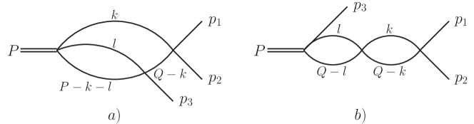
Figure 1: Two topologically distinct non-relativistic two-loop graphs describing the final-state $\pi\pi$ re-scattering in the decay $K\to 3\pi$, with $Q^{\mu}=(p_{1}+p_{2})^{\mu}$.

The non-trivial contribution from Fig. 1a is proportional to

$${\mathcal{M}}(s)=\int\frac{d^{D}l}{i(2\pi)^{D}}\,\frac{d^{D}k}{i(2\pi)^{D}}\,S_{a}(P-l-k)S_{b}(l)S_{c}(k)S_{d}(Q-k)$$ (12)

A short discussion of this integral is given in Ref. [6]. There, it is shown that one may write

$${\mathcal{M}}(s)=F\bigl{(}M_{a},M_{b},M_{c},M_{d};s\bigr{)}+\ldots,$$ (13)

where $F$ is ultraviolet finite and contains the full non-analytic behavior of the two-loop diagram in the low-energy domain, whereas the ellipsis denotes terms that amount to a redefinition of the tree-level couplings in ${\cal L}_{K},\bar{\cal L}_{K}$ and which are therefore dropped. A one-dimensional integral representation for $F$ is provided in Ref. [6]. The relevant integrals can be also performed analytically [7].

Finally, the diagram in Fig. 1b is a product of two one-loop diagrams given in Eq. (10).

3 Including photons

3.1 The Lagrangian with photons

In this and the following sections we discuss the inclusion of photons in the non-relativistic framework. Since power counting is more complicated in the presence of photons, we first consider examples of simple vertices and diagrams with photons, without trying to order them according to the power counting.

The kinetic part of the Lagrangian after minimal substitution takes the form

$${\cal L}_{\rm kin} =-\frac{1}{4}\,F_{\mu\nu}F^{\mu\nu}+\sum_{\pm}\Bigl{(}i\Phi_{\pm}^{\dagger}D_{t}{\cal W}_{\pm}\Phi_{\pm}-i(D_{t}{\cal W}_{\pm}\Phi_{\pm})^{\dagger}\Phi_{\pm}-2\Phi_{\pm}^{\dagger}{\cal W}_{\pm}^{2}\Phi_{\pm}\Bigr{)}$$

$$+2\Phi_{0}^{\dagger}W_{0}(i\partial_{t}-W_{0})\Phi_{0}+\Bigl{(}iK^{\dagger}D_{t}{\cal W}_{K}K-i(D_{t}{\cal W}_{K}K)^{\dagger}K-2K^{\dagger}{\cal W}_{K}^{2}K\Bigr{)}$$

$$+2K_{L}^{\dagger}\bar{W}_{K}(i\partial_{t}-\bar{W}_{K})K_{L}\,.$$ (14)

Here, $F_{\mu\nu}=\partial_{\mu}A_{\nu}-\partial_{\nu}A_{\mu}$ denotes the electromagnetic field strength tensor and

$$D_{t}\Phi_{\pm} =(\partial_{t}\mp ieA_{0})\Phi_{\pm}\,, D_{t}K =(\partial_{t}-ieA_{0})K\,,$$

$${\cal W}_{\pm} =\sqrt{M_{\pi}^{2}-{\bf D}^{2}}\,, {\cal W}_{K} =\sqrt{M_{K}^{2}-{\bf D}^{2}}\,,$$

$${\bf D}\Phi_{\pm} =(\nabla\pm ie{\bf A})\Phi_{\pm}\,, {\bf D}K =(\nabla+ie{\bf A})K\,.$$ (15)

In an explicit calculation of the tree-level photon-pion and photon-kaon vertices, the roots ${\cal W}_{\pm}$, ${\cal W}_{K}$ are understood to be expanded in the inverse of the corresponding mass. After resummation of all terms proportional to $e$, the relativistic result is explicitly reproduced at tree level,

$$\langle\pi^{\pm}(p^{\prime})|j_{\mu}^{\rm em}(0)|\pi^{\pm}(p)\rangle=\pm e(p^{\prime}+p)_{\mu}\,,~{}\langle K^{+}(p^{\prime})|j_{\mu}^{\rm em}(0)|K^{+}(p)\rangle=e(p^{\prime}+p)_{\mu}\,.$$ (16)

$j_{\mu}^{\rm em}$ denotes the electromagnetic current, calculated from the Lagrangian in a standard manner. Note that the non-relativistic Lagrangian Eq. (14) does not contain a term for pion pair creation by a photon, $\gamma\to\pi^{+}\pi^{-}$, which would involve a high-energy photon. This omission eliminates all one-photon reducible graphs from the $K\to 3\pi$ amplitudes considered in the following.

The spatial derivatives in the four-pion vertex are replaced by the covariant derivatives in the presence of photons. In addition, non-minimal terms, containing the electric ${\bf E}$ and magnetic ${\bf B}$ fields, will be present. At lowest order, the non-local coupling of the Coulomb photon field $A_{0}$ with e.g. the pion emerges, see Fig. 2. The pertinent coupling constant is proportional to the mean charge radius squared of the pion [30]. However, at the order we are working, this term in the Lagrangian can be eliminated by using the equations of motion and thus it does not affect any physical observable (we refer the interested reader to Ref. [30] for a detailed discussion of this issue). It can also be shown that higher-order non-minimal couplings do not contribute at the order we are working. In the following, we discard all non-minimal couplings in the Lagrangian from the beginning.

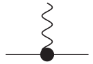
Figure 2: Effective-range coupling of the Coulomb photon to a charged pion. The coupling is proportional to the pion charge radius squared.

Further, we also discard the contribution arising from vacuum polarization generated by an electron-positron loop (see again Ref. [30]). We have checked that this correction is tiny and amounts to a few percent change of the (already small) Coulomb correction in the “auxiliary” decay modes.

The loop calculations in the non-relativistic theory are most easily done in the Coulomb gauge. Here, first the time component $A_{0}$ is removed from the Lagrangian by using the equations of motion. This procedure generates the non-local operator

$$\triangle^{-1}=-\int\frac{d^{3}{\bf k}}{(2\pi)^{3}}\,\frac{{\rm e}^{-i{\bf k}({\bf x}-{\bf y})}}{{\bf k}^{2}}$$ (17)

in the Lagrangian. In the following, for ease of understanding, we keep calling the pertinent diagrams as “generated by the exchange of Coulomb photons.” The propagator of the transverse photons in the Coulomb gauge is given by

$$D^{ij}(k)=i\int d^{4}x\,{\rm e}^{ikx}\langle 0|TA^{i}(x)A^{j}(0)|0\rangle=-\frac{1}{k^{2}}\,\biggl{(}\delta^{ij}-\frac{k^{i}k^{j}}{{\bf k}^{2}}\biggr{)}\,.$$ (18)

Below, the virtual photon corrections to the strong amplitudes are calculated at $\mathcal{O}(e^{2})$ (with the exception of the discussion in Sect. 6), i.e. we include one virtual photon at most. In order to obey counting rules, as in the purely strong case, one has to perform threshold expansions. In the following section we explain how this can be done on the basis of several examples. The counting rules in the presence of photons are discussed in full generality afterwards in Sect. 5.

3.2 Matching

The effective coupling constants in the Lagrangian can be related to physical observables in the underlying relativistic field theory. This procedure goes under the name of matching. Here, chiral perturbation theory is understood to be the underlying theory, which we bear in mind while performing the matching.

In order to determine the (four-pion) coupling constants in the non-relativistic theory through matching, one has to calculate the pion-pion scattering amplitude both in the non-relativistic theory and in the underlying theory. These amplitudes are then expanded in the pion momenta at threshold, and the pertinent expansion coefficients are set equal (up to a given order). One has to distinguish the isospin symmetry limit and the case with broken isospin symmetry.

3.2.1 Isospin symmetry limit

In the isospin symmetry limit, the expansion of the relativistic $\pi\pi$ scattering amplitude at threshold reads

$${\rm Re}\,\bar{T}_{i}(s,t)=\bar{A}_{i}+\mathcal{O}(\epsilon^{2})~{}.$$ (19)

The bar indicates the quantities in the isospin-symmetric world, in which the pion has the mass $M_{\pi}=139.57$ MeV. In terms of the standard scattering lengths $a_{0}$ and $a_{2}$, one has

$$3\bar{A}_{1} ={N(a_{0}+2a_{2})}\,, 2\bar{A}_{2} ={Na_{2}}\,, 3\bar{A}_{3} ={N(a_{2}-a_{0})}\,,$$

$$6\bar{A}_{4} ={N(2a_{0}+a_{2})}\,, \bar{A}_{5} =Na_{2}\,, N =32\pi\,\,,$$ (20)

with $a_{0}=0.220\pm 0.005$, $a_{2}=-0.0444\pm 0.0010$, $a_{0}-a_{2}=0.265\pm 0.004$ [21]. Still in the isospin symmetry limit, the couplings $C_{i}$ are related to these threshold parameters according to

$$2\bar{C}_{i}=\bar{A}_{i}\,\,\,,$$ (21)

where we have dropped higher-order terms in the threshold parameters.

We wish to note that the matching condition is universal in the isospin-symmetric case and determines the coupling constants in terms of the effective-range expansion parameters only. There is no explicit reference to the Lagrangian of the underlying relativistic theory.

3.2.2 Isospin-violating case

The isospin-breaking corrections to the isospin-symmetric result emerge from electromagnetic effects as well as from the up/down quark mass difference and have the following general form (see, e.g., Refs. [29, 30]):

$$C_{i}=\bar{C}_{i}+h_{1}(m_{d}-m_{u})^{2}+h_{2}e^{2}+\mathcal{O}(e^{4},e^{2}(m_{d}-m_{u})^{2},(m_{d}-m_{u})^{4})\,,$$ (22)

where the coefficients $h_{1,2}$ depend on the quark mass $\hat{m}=\frac{1}{2}\,(m_{u}+m_{d})$. Note that the corrections are no more universal, and in order to carry out the calculations, one has to use the explicit form of the underlying Lagrangian of the relativistic theory. Further, in order to perform the matching in the presence of photons, one has first to remove the infrared-singular piece of the amplitude at threshold. The procedure is described in Refs. [29, 30] and will not be repeated here.

At leading order in chiral perturbation theory one finds [34, 29]

$$2C_{1,2,5}=\bar{A}_{1,2,5}(1-\eta),\,\,2C_{3}=\bar{A}_{3}(1+\eta/3),\,\,2C_{4}=\bar{A}_{4}(1+\eta),$$ (23)

where $\eta=(M_{\pi}^{2}-M_{\pi^{0}}^{2})/M_{\pi}^{2}=6.5\times 10^{-2}$.

The calculations at one-loop level have been carried out, in particular, for the process $\pi^{+}\pi^{-}\to\pi^{0}\pi^{0}$ that multiplies the cusp in the $K\to 3\pi$ decays at lowest order. The final result can be extracted, e.g., from Eqs. (4.14), (4.28) and (4.29) of Ref. [29],

$$2C_{3} = -\frac{32\pi}{3}\bigl{[}a_{0}-a_{2}+(0.61\pm 0.16)\times 10^{-2}\bigr{]}$$ (24)

$$= \bar{A}_{3}\,(1+(2.3\pm 0.6)\times 10^{-2})\,,$$

where in the second line we have used $a_{0}-a_{2}=0.265$. The bulk of the total correction is already given by the tree-level result in Eq. (23), and most of the uncertainty stems from the so-called “electromagnetic” low-energy constants in the $\mathcal{O}(e^{2}p^{2})$ chiral Lagrangian [34]. The higher-order corrections to the matching of $C_{1,2,4,5}$ are less important, because these couplings enter the cusp amplitude at the sub-leading order. In general, one may conclude that isospin-breaking corrections beyond tree level – given in Eq. (23) – amount to a systematic uncertainty in the $C_{i}$ at the percent level.

4 Examples of loop calculations with photons

4.1 Ultraviolet and infrared divergences: general remarks

The loop diagrams with photons in the non-relativistic EFT have both ultraviolet and infrared divergences. Their treatment is different: whereas the ultraviolet divergences are removed by renormalization, the infrared ones cancel in the total decay rate, including the decay into soft photons. Further, the non-relativistic EFT exactly reproduces the structure of the infrared divergences in the underlying relativistic theory. On the other hand, the high-energy behavior in these two theories, in general, differs.

Throughout this paper, we tame both ultraviolet and infrared divergences by dimensional regularization. In addition, the threshold expansion is used in the Feynman integrals in order to ensure the validity of the counting rules in the presence of photons. One has to face, however, the following problem. Both ultraviolet and infrared divergences show up as poles in the amplitudes in the variable $D$ as $D\to 4$. The origin of the singularity (either ultraviolet or infrared) can be easily identified, and one may attach a subscript to these poles, writing $\left(\frac{1}{D-4}\right)_{UV}$ and $\left(\frac{1}{D-4}\right)_{IR}$ explicitly. At the order we are working, it can be checked that, if threshold expansion is not applied, the infrared poles that emerge in the non-relativistic EFT, as expected, are identical to those in the pertinent graphs of the underlying relativistic theory.

However, the threshold expansion generally changes the behavior of the diagrams in the infrared, and the structure of the infrared poles does not match the underlying theory anymore. In order to see this, we note that applying threshold expansion and the subsequent use of the no-scale argument in dimensional regularization amounts to the replacement

$$\left(\frac{1}{D-4}\right)_{UV}-\left(\frac{1}{D-4}\right)_{IR}\to 0$$ (25)

in the pertinent terms. For more details, we refer the reader to Appendix E, where we illustrate the issue with the vertex diagram.

In this paper, we adopt the following simple solution of the problem. As becomes clear from the above expression, the coefficient of the infrared pole changes by a low-energy “polynomial” as a result of the threshold expansion. For this reason, we do not differentiate between infrared and ultraviolet divergences (detaching the subscripts “UV” and “IR” everywhere) and remove all remaining divergences by the counterterms of the Lagrangian in a threshold-expanded EFT. This leads to the correct result for all observables, since all infrared divergences cancel at the end.

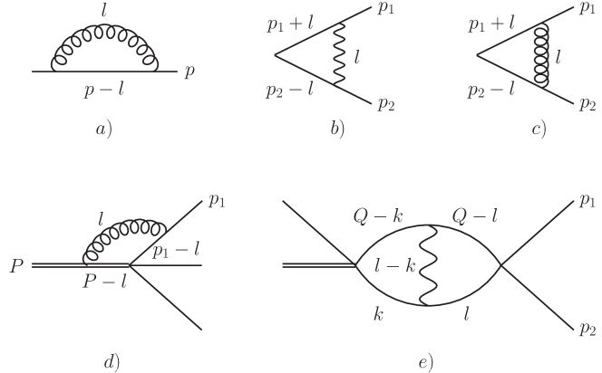
Figure 3: Examples of loop graphs with photons in the non-relativistic EFT. Double and single full lines denote kaons and pions, respectively, wiggly lines stand for Coulomb, curly lines for transverse photons. a: pion self-energy (transverse photon); b: vertex diagram with Coulomb photon; c: vertex diagram with transverse photon; d: vertex diagram in crossed channel (transverse photon); e: Coulomb photon exchange in the strong loop.

4.2 Self-energy of the pion

The self-energy diagram of the charged pion shown in Fig. 3a is given by the following integral

$$\Sigma(p)=\frac{e^{2}}{2w_{\pm}({\bf p})}\,\int\frac{d^{D}l}{i(2\pi)^{D}}\,S_{\pm}(p-l)\frac{(2p-l)^{i}(2p-l)^{j}}{-l^{2}}\biggl{(}\delta^{ij}-\frac{l^{i}l^{j}}{{\bf l}^{2}}\biggr{)}\,.$$ (26)

Only the transverse photons contribute.

In order to calculate $\Sigma(p)$, we perform the Cauchy integral over $l^{0}$ and further use the identity

$$\frac{1}{2w_{\pm}({\bf p}-{\bf l})}\,\frac{1}{w_{\pm}({\bf p}-{\bf l})-p^{0}+|{\bf l}|} =-\frac{1}{2w_{\pm}({\bf p}-{\bf l})}\,\frac{1}{w_{\pm}({\bf p}-{\bf l})+p^{0}-|{\bf l}|}$$

$$\quad+\frac{1}{w_{\pm}^{2}({\bf p}-{\bf l})-(p^{0}-|{\bf l}|)^{2}}\,.$$ (27)

Since both $w_{\pm}({\bf p}-{\bf l}),~{}p^{0}=\mathcal{O}(1)$ in the $\epsilon$ counting, the threshold expansion in the first term generates polynomials in the integration momenta. Using no-scale arguments, it is seen that the integral of the first term vanishes in dimensional regularization.

The denominator in the second term can be written as $\Omega+2p^{0}|{\bf l}|-2{\bf p}{\bf l}$, where $\Omega=w_{\pm}^{2}({\bf p})-(p^{0})^{2}=M_{\pi}^{2}-p^{2}=\mathcal{O}(\epsilon^{2})$. In order to expand the denominator, one has to establish the power counting rules for the photon 3-momentum ${\bf l}$. One observes that in this particular diagram ${\bf l}$ should be assigned the power $\mathcal{O}(\epsilon^{2})$, otherwise one arrives at no-scale integrals after expansion in $\epsilon$, which vanish in dimensional regularization. Assuming ${\bf l}=\mathcal{O}(\epsilon^{2})$ and expanding this denominator in the last term, which is of order $\epsilon^{3}$ (the first two terms are of order $\epsilon^{2}$), we find

$$\Sigma(p)=\frac{e^{2}{\bf p}^{2}}{2w_{\pm}({\bf p})p^{0}}\biggl{(}\frac{\Omega}{2p^{0}}\biggr{)}^{d-2}\Bigl{(}1-\frac{1}{d}\Bigr{)}\frac{2\pi^{d/2}}{(2\pi)^{d}\Gamma(\frac{d}{2})}\,\Gamma(d-1)\Gamma(2-d)+\ldots\,,$$ (28)

where $d=D-1$, and the ellipses stand for higher-order terms in the $\epsilon$-expansion. In the limit $d\to 3$ we obtain

$$\Sigma(p) =\frac{4e^{2}{\bf p}^{2}\Omega}{3w_{\pm}({\bf p})(p^{0})^{2}}\,\biggl{(}\lambda+\frac{1}{16\pi^{2}}\biggl{(}\ln\frac{\Omega}{\mu p^{0}}-\frac{1}{3}\biggr{)}\biggr{)}+\ldots\,,$$ (29)

$$\lambda =\frac{\mu^{D-4}}{16\pi^{2}}\,\biggl{(}\frac{1}{D-4}-\frac{1}{2}\,\bigl{(}\Gamma^{\prime}(1)+\ln 4\pi+1\bigr{)}\biggr{)}\,,$$ (30)

which is in perfect agreement with the standard non-relativistic framework (see e.g. Ref. [29]). Here $\mu$ denotes the scale of dimensional regularization. The divergence at $D\to 4$ is ultraviolet. However, as mentioned above, in the following we shall not distinguish between the ultraviolet and infrared poles. Note that, since this expansion does not move the location of the singularity in the self-energy fixed by the relativistic relation $p^{2}=M_{\pi}^{2}$, there is no need to eventually re-sum the obtained series.

The expression for the $Z$-factor of the charged pion can be directly obtained from Eq. (28) by performing the limit $\Omega\to 0$ at $d>3$ (see, e.g., Refs. [35, 30]). In this manner, one finds

$$Z=1\,.$$ (31)

4.3 Coulomb vertex

The Coulomb vertex, shown in Fig. 3b, is given by

$$V_{C} =-e^{2}\int\frac{d^{D}l}{i(2\pi)^{D}}\,S_{\pm}(p_{1}+l)S_{\pm}(p_{2}-l)\,\frac{(w_{1}+w_{1}^{\prime})(w_{2}+w_{2}^{\prime})}{{\bf l}^{2}}\,,$$

$$w_{1} =w_{\pm}({\bf p}_{1})\,,\quad w_{1}^{\prime}=w_{\pm}({\bf p}_{1}+{\bf l})\,,\quad w_{2}=w_{\pm}({\bf p}_{2})\,,\quad w_{2}^{\prime}=w_{\pm}({\bf p}_{2}-{\bf l})\,.$$ (32)

Performing the Cauchy integration over $l^{0}$ and using the threshold expansion, one can demonstrate that the numerator may be replaced by

$$(w_{1}+w_{1}^{\prime})(w_{2}+w_{2}^{\prime})\to 4w_{1}w_{2}-\biggl{(}\frac{w_{1}-w_{2}}{w_{1}+w_{2}}\,{\bf Q}+2{\bf q}\biggr{)}\,{\bf l}-{\bf l}^{2}\,,$$ (33)

with ${\bf Q}={\bf p}_{1}+{\bf p}_{2}$ and ${\bf q}=({\bf p}_{1}-{\bf p}_{2})/2$. Further, it can be checked that the energy denominator that emerges after integration over $l^{0}$ can be rewritten as

$$\frac{1}{2w_{1}^{\prime}2w_{2}^{\prime}}\,\frac{1}{w_{1}^{\prime}+w_{2}^{\prime}-E} =\frac{1}{2E}\,\frac{1}{{\bf l}^{2}+2{\bf b}{\bf l}-({\bf Q}{\bf l})^{2}/E^{2}-\lambda(E^{2},w_{1}^{2},w_{2}^{2})/4E^{2}}+\ldots\,,$$

$$E =w_{1}+w_{2}\,,\qquad{\bf b}={\bf q}-\frac{{\bf Q}({\bf Q}{\bf q})}{E^{2}}\,.$$ (34)

Using the substitution

$${\bf l}\to{\bf l}+\frac{{\bf Q}({\bf Q}{\bf l})}{\sqrt{s}(E+\sqrt{s})}-{\bf b}-\frac{{\bf Q}({\bf Q}{\bf b})}{s}\,,\quad\quad s=E^{2}-{\bf Q}^{2}=(p_{1}+p_{2})^{2}\,,$$ (35)

we may rewrite the integral as

$$V_{C}=-\frac{e^{2}}{2\sqrt{s}}\,\int\frac{d^{d}l}{(2\pi)^{d}}\,\frac{1}{{\bf l}^{2}-q_{0}^{2}}\,\frac{4M_{\pi}^{2}}{({\bf l}-q_{0}{\bf q}/|{\bf q}|)^{2}}+\ldots\,,\quad\quad q_{0}^{2}=\frac{s}{4}-M_{\pi}^{2}\,,$$ (36)

where the ellipses again represent higher-order terms in $\epsilon$. At lowest order in $\epsilon$ we obtain (cf.  e.g. Refs. [29, 30])

$$V_{C}=\frac{2\alpha M_{\pi}}{\sqrt{s}}\,\biggl{(}-\frac{\pi M_{\pi}}{4q_{0}}-i\theta_{c}(q_{0})+\mathcal{O}(d-3)\biggr{)}+\ldots\,,\quad q_{0}^{2}>0\,,$$ (37)

where $\alpha$ denotes the fine structure constant,

$$\theta_{c}(q_{0})=\frac{M_{\pi}}{2q_{0}}\biggl{(}16\pi^{2}\lambda+\frac{1}{2}\biggl{(}\ln\frac{4q_{0}^{2}}{\mu^{2}}+1\biggr{)}\biggr{)}+\ldots$$ (38)

is the (infrared-divergent) Coulomb phase, and the ellipses stand for higher-order terms in the expansion in $\epsilon$. Since these terms do not change the position of the branch point in the diagram at $s=4M_{\pi}^{2}$, there is no need to re-sum these terms.

From Eq. (36) we may observe that the counting of the photon momentum ${\bf l}=\mathcal{O}(\epsilon)$ is different from the case of the self-energy diagram.

4.4 Transverse vertex

The vertex with the transverse photon, which is shown in Fig. 3c, is suppressed by a factor $\epsilon^{2}$ as compared to the Coulomb vertex due to the derivative coupling of the transverse photons to pions. It is given by the following Feynman integral

$$V_{T}=-e^{2}\int\frac{d^{D}l}{i(2\pi)^{D}}\,S_{\pm}(p_{1}+l)S_{\pm}(p_{2}-l)\,\frac{(2p_{1}+l)^{i}(2p_{2}-l)^{j}}{l^{2}}\,\biggl{(}\delta^{ij}-\frac{l^{i}l^{j}}{{\bf l}^{2}}\biggr{)}\,.$$ (39)

Below, instead of $V_{T}$, we shall present the result for $V_{C}+V_{T}$. Applying threshold expansion, it can be shown that the sum of Coulomb and transverse vertices can be rewritten as

$$V_{C}+V_{T}=e^{2}\int\frac{d^{D}l}{i(2\pi)^{D}}\,S_{\pm}(p_{1}+l)S_{\pm}(p_{2}-l)\,\frac{4p_{1}p_{2}+l^{2}}{l^{2}}\,.$$ (40)

Using the same technique as in the case of the Coulomb vertex, we finally obtain a compact expression valid to all orders in the $\epsilon$-expansion,

$$V_{C}+V_{T} =-\frac{2\alpha\,p_{1}p_{2}}{M_{\pi}\sqrt{s}}\biggl{(}\frac{\pi M_{\pi}}{4q_{0}}+i\theta_{c}(q_{0})\biggr{)}+\frac{i\alpha q_{0}}{2\sqrt{s}}+\mathcal{O}(d-3)\,$$

$$=-\alpha\biggl{\{}\frac{\pi(1+\sigma^{2})}{4\sigma}+i\biggl{(}\frac{1+\sigma^{2}}{\sqrt{1-\sigma^{2}}}\,\theta_{c}(q_{0})-\frac{\sigma}{4}\biggr{)}\biggr{\}}+\mathcal{O}(d-3)\,,$$ (41)

where in the second line, we have introduced $\sigma=\sqrt{1-4M_{\pi}^{2}/s}$. As in the Coulomb vertex, the photon 3-momentum in the loop ${\bf l}$ counts as $\mathcal{O}(\epsilon)$. Note that $V_{C}+V_{T}$ is explicitly Lorentz-covariant. Equation (41) can also be derived in the formalism of Refs. [32, 33], see Ref. [36].

4.5 Transverse vertex in crossed channel

The vertex in which one of the photon lines is attached to the incoming kaon line is depicted in Fig. 3d. Neglecting all factors in the numerator, we consider the following scalar integral

$$V_{K}=e^{2}\int\frac{d^{D}l}{i(2\pi)^{D}}\,S_{\pm}(p_{1}-l)S_{K}(p_{K}-l)\frac{1}{-l^{2}}\,.$$ (42)

After integrating over $l^{0}$ we find

$$V_{K}=e^{2}\int\frac{d^{d}l}{(2\pi)^{d}}\,\frac{1}{2w_{1}^{\prime}2w_{K}^{\prime}}\,\frac{1}{2|{\bf l}|}\,\frac{1}{(w_{1}^{\prime}-w_{1}+|{\bf l}|)(w_{K}^{\prime}-w_{K}+|{\bf l}|)}\,,$$ (43)

where $w_{1}^{\prime}=w_{\pm}({\bf p}_{1}-{\bf l})$, $w_{1}=w_{\pm}({\bf p}_{1})$, $w_{K}^{\prime}=w_{K}({\bf p}_{K}-{\bf l})$ and $w_{K}=w_{K}({\bf p}_{K})$. From Eq. (43) one concludes that the photon momentum ${\bf l}$ has to be counted as $\mathcal{O}(\epsilon^{2})$. However, since

$$w_{1}^{\prime}-w_{1}+|{\bf l}|=|{\bf l}|-\frac{{\bf p}_{1}{\bf l}}{w_{1}}+\ldots\,,\quad\quad w_{K}^{\prime}-w_{K}+|{\bf l}|=|{\bf l}|-\frac{{\bf p}_{K}{\bf l}}{w_{K}}+\ldots\,,$$ (44)

and since the second term in this expansion counts as $\mathcal{O}(\epsilon^{3})$, we arrive at no-scale integrals. Consequently, we conclude that $V_{K}=0$; see also the discussion in Appendix E.

4.6 Coulomb exchange in strong loops

The exchange of a Coulomb photon in the strong loop (see Fig. 3e) is described by the following integral:

$$J_{C}=e^{2}\int\frac{d^{D}l}{i(2\pi)^{D}}\,\frac{d^{D}k}{i(2\pi)^{D}}\,S_{\pm}(l)S_{\pm}(Q-l)S_{\pm}(k)S_{\pm}(Q-k)\,\frac{(w_{1}^{\prime}+w_{1}^{\prime\prime})(w_{2}^{\prime}+w_{2}^{\prime\prime})}{|{\bf l}-{\bf k}|^{2}}\,,$$ (45)

where $Q=p_{1}+p_{2}$, $w_{1}^{\prime}=w_{\pm}({\bf l})$, $w_{2}^{\prime}=w_{\pm}({\bf Q}-{\bf l})$, $w_{1}^{\prime\prime}=w_{\pm}({\bf k})$, and $w_{2}^{\prime\prime}=w_{\pm}({\bf Q}-{\bf k})$. Replacing $(w_{1}^{\prime}+w_{1}^{\prime\prime})(w_{2}^{\prime}+w_{2}^{\prime\prime})=2w_{1}w_{2}+\mathcal{O}(\epsilon^{2})$, where $w_{1}=w_{\pm}({\bf p}_{1})$ and $w_{2}=w_{\pm}({\bf p}_{2})$, integrating over $l^{0}$, $k^{0}$ and re-defining the integration 3-momenta ${\bf l}$, ${\bf k}$ along similar lines as in Sect. 4.3, we finally find

$$J_{C}=\frac{e^{2}M_{\pi}^{2}}{s}\,\int\frac{d^{d}l}{(2\pi)^{d}}\,\frac{d^{d}k}{(2\pi)^{d}}\,\frac{1}{{\bf l}^{2}-q_{0}^{2}}\,\frac{1}{|{\bf l}-{\bf k}|^{2}}\,\frac{1}{{\bf k}^{2}-q_{0}^{2}}+\ldots\,,$$ (46)

where $q_{0}^{2}=s/4-M_{\pi}^{2}$ and $s=Q^{2}$. From the above expression it is seen that ${\bf l},{\bf k}$ count as $\mathcal{O}(\epsilon)$. The higher-order corrections in Eq. (46) do not change the location of the threshold given by the relativistically invariant relation $s=4M_{\pi}^{2}$.

Calculating the integral in Eq. (46), we arrive at

$$J_{C}=-\frac{\alpha M_{\pi}^{2}}{8\pi s}\,\biggl{(}16\pi^{2}\Lambda+\ln\Bigl{(}-\frac{4q_{0}^{2}}{\mu^{2}}\Bigr{)}\biggr{)}+\ldots\,,$$ (47)

where

$$\Lambda=\frac{\mu^{2(D-4)}}{16\pi^{2}}\biggl{(}\frac{1}{D-4}-\Gamma^{\prime}(1)-\ln 4\pi-1\biggr{)}\,.$$ (48)

5 Power counting

We start by summarizing the power counting rules for $K\to 3\pi$ decays without photons.

1. Polynomial interaction terms can be organized in even powers of $\epsilon$, starting at $\epsilon^{0}$. The inclusion of higher-order derivative terms in loop diagrams increases the power of $\epsilon$ of the respective graphs accordingly.

2. In loop diagrams, each pion propagator counts as $\epsilon^{-2}$, each loop integration as $\epsilon^{5}$ (as for an integration momentum $l$, $d\mathbf{l}=\mathcal{O}(\epsilon)$ and $dl^{0}=\mathcal{O}(\epsilon^{2})$).

3. Each loop formed with two-body rescattering terms (counted as $\mathcal{O}(a)$) therefore increases the power of $\epsilon$ by $\epsilon^{5}(\epsilon^{-2})^{2}=\epsilon^{1}$, therefore one-loop diagrams are $\mathcal{O}(a^{1}\epsilon^{1})$, two-loop diagrams $\mathcal{O}(a^{2}\epsilon^{2})$, etc. Loops with three-body terms increase the power of $\epsilon$ by $(\epsilon^{5})^{2}(\epsilon^{-2})^{3}=\epsilon^{4}$.

The examples of the preceding section show how these rules have to be amended in the presence of (virtual) photons. Note that, as $M_{\pi}^{2}-M_{\pi^{0}}^{2}=\mathcal{O}(e^{2})$ (when neglecting a tiny contribution of second order in the light quark mass difference), one might infer that the electric coupling should be included in a unified power counting, where $e=\mathcal{O}(\epsilon)$. However, we do not follow this approach, but instead count $e$ as a separate expansion parameter, such that we will altogether have a three-fold expansion in $\epsilon$, $a$, and $e$. In the following, we have to distinguish between “soft” photons ($l_{0}=\mathcal{O}(\epsilon^{2})$, $\mathbf{l}=\mathcal{O}(\epsilon)$) and “ultrasoft” photons ($l_{0}=\mathcal{O}(\epsilon^{2})$, $\mathbf{l}=\mathcal{O}(\epsilon^{2})$).

1. Coulomb photons are always soft, hence their propagators are $\mathcal{O}(\epsilon^{-2})$, and loop integration still counts as $\epsilon^{5}$. Furthermore, the couplings to bosons are of $\mathcal{O}(\epsilon^{0})$. The addition of a Coulomb photon to a “skeleton” diagram, consisting only of interaction vertices without electromagnetism, hence changes the non-relativistic power of the diagram by a factor of $\epsilon^{5}(\epsilon^{-2})^{3}=\epsilon^{-1}$. The two most relevant examples for $K\to 3\pi$ decays discussed individually above are the vertex correction with a Coulomb photon, Sect. 4.3, and Coulomb exchange within charged pion loops, Sect. 4.6.

2. Soft transverse photons have couplings of $\mathcal{O}(\epsilon^{1})$, hence the exchange of transverse photons is suppressed by two orders with respect to the corresponding Coulomb exchange diagram. An example for this is given in Sect. 4.4.

3. For ultrasoft transverse photons, with all momentum components of order $\epsilon^{2}$, the propagator counts as $\epsilon^{-4}$ and loop integration as $\epsilon^{8}$. Therefore, adding an ultrasoft transverse photon to a skeleton diagram changes its power counting by a factor of (taking care of loop integration, boson propagators, photon propagator, and photon vertices) $\epsilon^{8}(\epsilon^{-2})^{2}\epsilon^{-4}\epsilon^{2}=\epsilon^{2}$. Examples are the pion self-energy (Sect. 4.2) and the exchange of a transverse photon in the crossed channel (Sect. 4.5).

As the addition of a Coulomb photon modifies the power counting of a given diagram by a factor of $e^{2}/\epsilon$, it is obvious that we can consider very small momenta for which this ratio ceases to be a small parameter. This is precisely what happens in the energy region where pionium bound states are formed and will be discussed in detail in Sect. 6. The scheme formulated above holds outside a small energy window around the pionium singularities, where then the standard perturbative treatment of electromagnetism is valid.

As the inclusion of real photon radiation effects takes place on the level of widths or decay spectra, we briefly discuss the non-relativistic power counting for both non-radiative and radiative widths/decay spectra. The non-radiative differential decay width $d\Gamma$ for $K\to 3\pi$ is schematically given by

$$d\Gamma~{}\propto~{}\Bigl{[}\prod d\mu(p_{i})\Bigr{]}\delta^{(4)}\Bigl{(}P-\sum p_{i}\Bigr{)}|\mathcal{M}|^{2}~{},~{}~{}d\mu(p_{i})=\frac{d^{3}p_{i}}{2p_{i}^{0}(2\pi)^{3}}~{}.$$ (49)

Each invariant phase space element counts according to $d\mu(p_{i})\propto\epsilon^{3}$, while the energy- and momentum-conserving $\delta$-function induces a factor of $\epsilon^{-5}$. With the matrix element $\mathcal{M}$ starting at $\mathcal{O}(\epsilon^{0})$, it is therefore obvious that the non-radiative differential decay width starts out as $\mathcal{O}(\epsilon^{4})$, and the decay spectrum with respect to $s_{3}$ obeys

$$\frac{d\Gamma}{ds_{3}}~{}=~{}\mathcal{O}(\epsilon^{2})~{}.$$ (50)

The radiative differential decay width $d\Gamma_{\gamma}$ is schematically given by

$$d\Gamma_{\gamma}~{}\propto~{}\Bigl{[}\prod d\mu(p_{i})\Bigr{]}d\mu(k)\delta^{(4)}\Bigl{(}P-\sum p_{i}-k\Bigr{)}|\mathcal{M}_{\gamma}|^{2}~{},~{}~{}d\mu(k)=\frac{d^{3}k}{2k^{0}(2\pi)^{3}}~{}.$$ (51)

Real photons necessarily are ultrasoft, as the energy component is $k^{0}=\mathcal{O}(M_{K}-3M_{\pi})=\mathcal{O}(\epsilon^{2})$, and the on-shell condition enforces the same order for the three-momentum components. Therefore the additional integration over the photon phase space is $d\mu(k)=\mathcal{O}(\epsilon^{4})$. The non-relativistic power counting for the radiative matrix element is most easily seen in the Coulomb gauge, where the matrix element for photon radiation (with momentum $k$) off the external legs (with charges $Q_{i}$, masses $M_{i}$, and momenta $p_{i}$) is given by

$$\mathcal{M}_{\gamma}~{}\propto~{}e\sum Q_{i}\frac{\mathbf{p}_{i}\boldsymbol{\epsilon}^{*}}{M_{i}k^{0}}\bigl{(}1+\mathcal{O}(\epsilon)\bigr{)}~{}=~{}\mathcal{O}\Bigl{(}\frac{e}{\epsilon}\Bigr{)}~{}.$$ (52)

Combining Eqs. (51), (52), we obtain $d\Gamma_{\gamma}=\mathcal{O}(e^{2}\epsilon^{6})$ and

$$\frac{d\Gamma_{\gamma}}{ds_{3}}~{}=~{}\mathcal{O}(e^{2}\epsilon^{4})~{}.$$ (53)

We find therefore that, for the projected accuracy, it is sufficient to calculate bremsstrahlung effects at leading non-vanishing order in the non-relativistic expansion.

The following conclusions can furthermore be drawn.

1. As the relation between the (massive boson) propagators in the relativistic and the non-relativistic theories is given by

   $$\frac{1}{p^{2}-M^{2}}~{}=~{}\frac{1}{2\omega(\mathbf{p})(p^{0}-\omega(\mathbf{p}))}+\mathcal{O}(\epsilon^{0})~{},$$

   a calculation of the real photon radiation effects in both theories is equivalent up to the desired order. We can therefore simply expand the relativistic results in $\epsilon$.

2. Contributions to the radiative width that are not of bremsstrahlung type, i.e. the photon is not attached to one of the external legs, is further suppressed in the $\epsilon$-expansion and does not need to be considered.

3. The same goes for bremsstrahlung type contributions with derivative vertices or loops, which are also of subleading order in the $\epsilon$-expansion.

At the end of this section, we can summarize our conclusions from the above considerations by discussing the Feynman graphs for all real and virtual photon corrections necessary for a consistent calculation of $d\Gamma/ds_{3}$ up-to-and-including $\mathcal{O}(e^{2}a^{0}\epsilon^{4})$ (all channels) and $\mathcal{O}(e^{2}a^{1}\epsilon^{2})$ (for the “main modes” only).

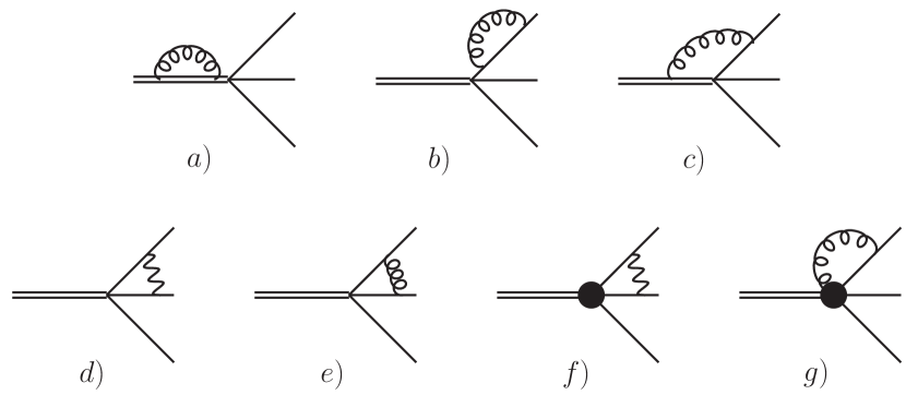
Figure 4: Representative set of one-loop diagrams for $K\to 3\pi$ including a virtual photon. Double, single, wiggly, and curly lines denote kaons, pions, Coulomb, and transverse photons, respectively. The thick blob denotes an interaction vertex with two derivatives.

Virtual photon corrections suppressed with respect to leading tree terms by factors up to $\mathcal{O}(e^{2}\epsilon^{2})$, i.e. without any $\pi\pi$ rescattering contributions, are shown in Fig. 4. According to the counting rules spelt out above, the transverse photon diagrams Fig. 4a–c are all of the maximal order we consider here, so no further derivative vertices have to be taken into account for the same diagram topologies. We need to consider both diagram Fig. 4d for Coulomb ($\mathcal{O}(e^{2}\epsilon^{-1})$) and Fig. 4e for transverse ($\mathcal{O}(e^{2}\epsilon^{1})$) photons. Coulomb exchange also necessitates the calculation of the same graph with a two-derivative vertex, Fig. 4f, which is then also of $\mathcal{O}(e^{2}\epsilon^{1})$. We furthermore wish to point out that no diagrams with photons coupling to interaction vertices, see Fig. 4g for an example, need to be considered, as those necessarily contain transverse photons with derivative interactions and therefore only start to contribute at $\mathcal{O}(e^{2}\epsilon^{4})$.

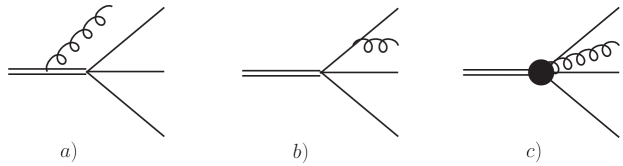
Figure 5: Diagrams for the bremsstrahlung process $K\to 3\pi\gamma$. The line style is as in Fig. 4.

The bremsstrahlung diagrams are displayed in Fig. 5. As argued above, only their leading order in $\epsilon$ contributes to $d\Gamma/ds_{3}$ at $\mathcal{O}(e^{2}\epsilon^{4})$, therefore no diagrams with additional derivative vertices are needed. In particular, structure-dependent photon radiation as in the graph Fig. 5c is suppressed by the absence of a meson propagator and the derivative in the vertex by at least two orders in $\epsilon$.

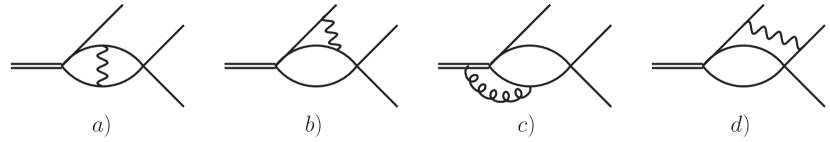
Figure 6: Two-loop diagrams for $K\to 3\pi$, including a virtual photon and one $\pi\pi$ rescattering vertex. Line style as in Fig. 4.

Finally, we turn to the diagrams that contain one further $\pi\pi$ interaction vertex, i.e. that are of $\mathcal{O}(e^{2}a^{1}\epsilon^{0})$. These are displayed in Fig. 6. Note that we only consider these corrections for the two “main modes” $K_{L}\to 3\pi^{0}$ and $K^{+}\to\pi^{0}\pi^{0}\pi^{+}$. Obviously, the diagram Fig. 6a (discussed extensively in Sect. 4.6 and below in Sect. 6) is the only one contributing to the former, and neither of the “main modes” features the topology shown in Fig. 6d (which requires at least two charged pions in the final state). As the pion loop as such is of $\mathcal{O}(\epsilon)$, only the addition of a Coulomb photon can lead to the required order in the non-relativistic counting, and transverse photon contributions like Fig. 6c are of higher order and can be neglected. Finally, the graph shown in Fig. 6b could potentially contribute to $K^{+}\to\pi^{0}\pi^{0}\pi^{+}$, with a $\pi^{+}\pi^{-}$ pair in the loop rescattering into $\pi^{0}\pi^{0}$. However, it is easily seen that the two contributions with the photon hooked to the $\pi^{+}$ and the $\pi^{-}$ in the loop exactly cancel, hence we do not have to consider this diagram either. We conclude that the graph discussed in Sect. 4.6 is indeed the only one at $\mathcal{O}(e^{2}a^{1}\epsilon^{0})$ that needs to be taken into account.

6 Pionium

In previous sections, we have analyzed the effect of radiative corrections in the perturbative regime, where an expansion in the fine structure constant $\alpha$ makes sense. In that region, pion momenta are counted as order $\epsilon$. Here, we investigate a region in momentum space where this is not necessarily true anymore: very near the cusp, pionium can form, and an expansion in $\alpha$ is obviously not possible. The three-momenta of pions are of order $\alpha$, and one needs to take into account an infinite number of graphs to describe this momentum regime properly.

There are two possibilities to cope with this problem. Either, one attempts to set up a formalism that allows one to treat the whole decay region, including the formation of pionium, in a coherent and consistent manner. Or, one proceeds in the manner in which the data analysis was performed by the NA48/2 collaboration [9]: one excludes a region around the cusp where this phenomenon occurs, and restricts the analysis to the region where a perturbative expansion in $\alpha$ is possible. We adopt this route in this article, for the following reason. Even if one might be able to set up a coherent formalism for the whole decay region, there would be no real benefit of such a tour de force in the present context: as we are interested in a precise extraction of the $\pi\pi$ scattering lengths, it is sufficient to stay in a region in momentum space where a perturbative treatment is possible, and where the effect of the cusp still allows one to extract the scattering lengths with high precision. Investigating the region where pionium is formed would then not provide any new information on the scattering lengths, but merely test the formalism to describe that region in a proper manner. This is so, because the energy resolution in present investigations of $K\to 3\pi$ decays does by far not suffice to e.g. measure the width of the ground state of pionium, which is an alternative possibility to measure $\pi\pi$ scattering lengths. In our opinion, this alternative way is best covered by dedicated measurements of the production and decay of pionium as performed e.g. in the DIRAC experiment [18, 19]. Here, the theoretical background for the data analysis has already been provided with the necessary precision [40, 41, 42, 43].

In the data analysis of NA48/2 [9], a region around the cusp was omitted,

$$s_{i}\not\in[4M_{\pi}^{2}-\Delta_{s},4M_{\pi}^{2}+\Delta_{s}]\,\,;\,\,\quad\Delta_{s}=5.25\times 10^{-4}\,\mbox{GeV}^{2}\,\,,$$ (54)

whenever $s_{i}$ corresponds to a channel where pionium can be formed. It therefore remains to answer the following question: is the region outside this interval accessible to a perturbative expansion in $\alpha$? As Ref. [9] has already demonstrated that this region does allow a precise measurement of the $\pi\pi$ scattering length (in the absence of radiative corrections), one is done once one knows that this question can be answered in a positive sense. The present section is devoted to an investigation of this problem.

6.1 $K_{L}\to 3\pi^{0}$

It is useful to start with the decay $K_{L}\to 3\pi^{0}$, because, as was shown at the end of the previous section, the graph Fig. 6a is the only one that needs to be taken into account in the perturbative region at order $\mathcal{O}(e^{2}a^{1}\epsilon^{0})$. It was evaluated in the present framework in Sect. 4.6. In the non-perturbative region, at order $a$, there are additional Coulomb exchanges that must be taken into account, see Fig. 7 for an example.

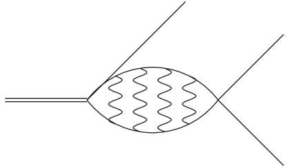
Figure 7: Diagram with four Coulomb photons exchanged between the oppositely charged pions. The quantity $J_{nC}$ in Eq. (6.1) describes the sum of diagrams with $n\geq 2$ Coulomb photon exchanges.

The effect of these Coulomb exchanges is to modify the one-loop integrals $J_{+-}(s)$ displayed in Eq. (10), in the following manner,

$$J_{+-}(s) \to J_{+-}(s)+J_{C}(s)+J_{nC}(s)\,.$$ (55)

Here, the second term on the right-hand side denotes the contribution of Fig. 6a. At the order considered here, it is given by

$$J_{C}(s)=-\frac{\alpha}{32\pi}\left(16\pi^{2}\Lambda+\ln{\Bigl{(}-\frac{4q_{0}^{2}}{\mu^{2}}\Bigr{)}}\right)\,;\,q_{0}^{2}=\frac{s}{4}-M_{\pi}^{2}\,.$$ (56)

The third term on the right-hand side of Eq. (55) stands for the sum of $n\geq 2$ Coulomb photon exchanges [44],

$$J_{nC} = -\frac{\alpha}{16\pi}\left(\Psi(1-\nu)-\Psi(1)\right)\,,$$

$$\nu = \frac{\alpha M_{\pi}}{2\sqrt{-q_{0}^{2}}}\,,\,\Psi(x)=\frac{d}{dx}\ln{\Gamma(x)}\,.$$ (57)

Two remarks are in order. First, the ultraviolet contribution that shows up in $J_{C}(s)$ can be absorbed in the couplings at tree level. In the following, we set the scale at $\mu=M_{\pi}$, and use instead of $J_{C}$ the expression

$$J_{C}\to\bar{J}_{C}=-\frac{\alpha}{32\pi}\ln{\left(-\frac{4q_{0}^{2}}{M_{\pi}^{2}}\right)}\,.$$ (58)

The choice of the scale is irrelevant: a change of scale simply induces a corresponding change in the tree-level couplings. Second, we performed the evaluation of $J_{nC}$ in the non-relativistic framework described in Ref. [29, 30], which differs from the one proposed here by use of propagators where the non-relativistic expansion $w_{\pm}(\mathbf{p})\to M_{\pi}+{\mathbf{p}^{2}}/{2M_{\pi}}+\cdots$ is performed. A calculation with the propagators used here would be rather demanding. On the other hand, that calculation would lead to the same result at leading order in the momentum expansion. As we shall drop the contributions from multi-Coulomb exchanges anyhow, see below, we do not attempt to perform this considerably more complicated calculation.

The effects of the non-perturbative regime is clearly seen in the multi-Coulomb contribution $J_{nC}$. Indeed, once the pion momenta count as order $\alpha$, $\nu$ is of order 1, and a perturbative expansion is no longer possible. A result of this are the pionium poles that show up in $J_{nC}$, at

$$q_{0}^{2}=-\frac{\alpha^{2}M_{\pi}^{2}}{4n^{2}}\,\,\,;\,\,n=1,2,\ldots\,.$$ (59)

On the other hand, this phenomenon only happens for pion momenta that are sufficiently small. Expanding $\Psi(1-\nu)$ around $\nu=0$, it is seen that multi-Coulomb exchanges are certainly negligible in comparison to the leading term $\bar{J}_{C}$ in case that the width of the cut satisfies $\Delta_{s}\geq 10^{-4}$ GeV². As a result of this, Coulomb exchanges finally amount to the replacement

$$J_{+-}(s) \to J_{+-C}(s)=J_{+-}(s)+\bar{J}_{C}(s)\,.$$ (60)

In the following, only the combination $J_{+-C}(s)$ will appear.

We now investigate the size of the one-Coulomb exchange at order $a$ and $a^{2}$. We drop contributions from derivative interactions in the matrix element and evaluate the ratio

$$R=\frac{\frac{d\Gamma}{ds_{3}}^{\rm{int}}-\frac{d\Gamma}{ds_{3}}^{0}}{\frac{d\Gamma}{ds_{3}}^{0}}\,.$$ (61)

The quantity $\frac{d{\Gamma}}{ds_{3}}^{\rm{int}}$ is calculated with the replacement Eq. (60). We first consider the case where this replacement is performed at one-loop order only. Charged pion loops then generate the two graphs displayed in Fig. 8. On the other hand, the Coulomb contributions $\bar{J}_{C}$ are dropped in $\frac{d\Gamma}{ds_{3}}^{0}$. The decay spectrum is calculated by use of the procedure described in Appendix F. The result for the ratio $R$ is displayed in Fig. 9, with a solid line, with tree-level couplings $L_{0}=-1.4K_{0}$, see Eq. (2.2). The grey band denotes the region discarded in the NA48/2 analysis. It is seen that outside this region, the correction due to one-Coulomb exchanges is of the order of one percent or less. Note that the ratio $R$ is linear in the ratio ${L_{0}}/{K_{0}}$ to very high accuracy.

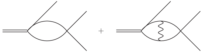
Figure 8: A contribution to the ratio $R$ in Eq. (61), evaluated with the replacement Eq. (60) at one-loop order. The pertinent $R$ is displayed in Fig. 9 with a solid line.

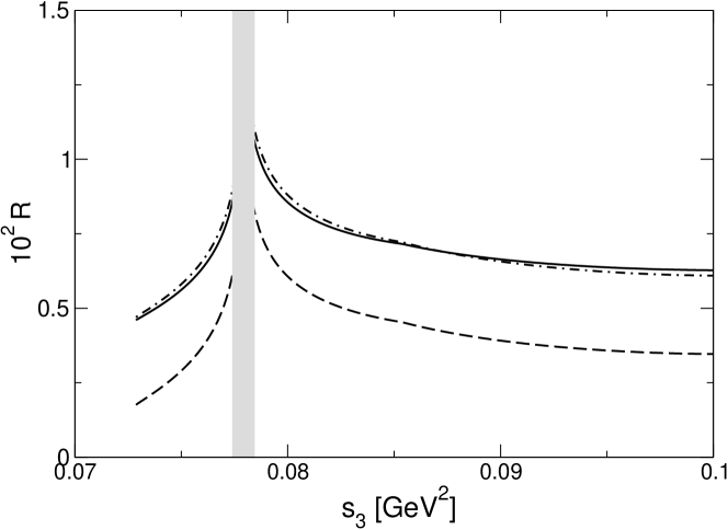
Figure 9: The effect of one-Coulomb exchanges in the spectrum of $K_{L}\to 3\pi^{0}$ decays. Shown is the ratio $R$ from Eq. (61). The grey band denotes the region Eq. (54), excluded in the data analysis of Ref. [9]. The solid line is evaluated with the replacement Eq. (60) at one-loop order. The dashed line corresponds to the same ratio, with the replacement Eq. (60) in bubble graphs at order $a$ and $a^{2}$. The dashed-dotted line illustrates that the effect of Coulomb exchanges at order $\alpha a^{2}$ can be removed to a large extent through a renormalization of the coupling $K_{0}$ in Eq. (2.2).

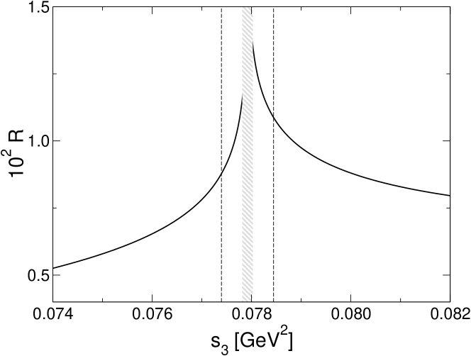
Figure 10: The effect of one-Coulomb exchanges inside the region Eq. (54) cut out in the NA48 analysis. The solid line again shows the ratio $R$ at one-loop order, discussed in the text. The dashed vertical lines indicate the region Eq. (54), whereas the hatched grey band denotes the same region, decreased by a factor of 5.

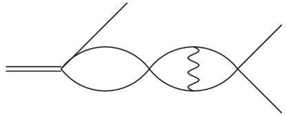
Figure 11: Contributions to the ratio $R$ at two-loop order. In graphs with charged pion loops, one additional Coulomb exchange is retained. The corresponding ratio $R$ in Eq. (61) is displayed in Fig. 9, with a dashed line.

We may also investigate $R$ closer to the position of the pionium poles. In Fig. 10 we display the ratio $R$ again, now also inside the region cut in the NA48/2 analysis. The grey vertical band corresponds to $s_{3}\not\in[4M_{\pi}^{2}-{\Delta_{s}/5},4M_{\pi}^{2}+{\Delta_{s}/5}]$, i.e., the excluded region Eq. (54) is reduced by a factor 5. The dashed vertical lines correspond to the original cut Eq. (54). It is seen that also in this enlarged region of phase space, the electromagnetic corrections due to one-Coulomb exchanges remain small.

We now comment on effects at order $\mathcal{O}(e^{2}a^{2}\epsilon)$ – a contribution at this order is e.g. generated by the graph displayed in Fig. 11. A full calculation of all pertinent graphs would be very complicated. For example, one would have to consider Coulomb photon exchanges in the two-loop graph displayed in Fig. 1a – a tremendous calculation. In order to have at least an order-of-magnitude estimate of the effect of these contributions, we perform the replacement Eq. (60) in bubble graphs at one- and two-loop order. The result for the ratio $R$ is shown in Fig. 9, with a dashed line. It is seen that the change in $R$ is rather substantial. However, almost all of this change can be absorbed in a redefinition of the coupling $K_{0}$ in Eq. (2.2). This is illustrated with the dash-dotted line in the same figure, which results from the dashed one by changing $K_{0}$ by half a percent, and which illustrates that the apparent sensitivity on the terms of order $\alpha a^{2}$ is of no concern in this region of momentum space.

6.2 $K^{+}\to\pi^{0}\pi^{0}\pi^{+}$

The discussion in this channel is analogous to the purely neutral channel just considered. We have checked that the corresponding ratio $R$ – see Eq. (61) – has qualitatively the same behavior as is shown in Figs. 9 for the purely neutral channel, although with smaller absolute value. Furthermore, a renormalization of the tree-level coupling again allows one to remove most of the contributions at order $\alpha a^{2}$.

We come to the following conclusions. The Coulomb corrections in hadronic loops are perturbative at least in the region which is used in the present data analysis by NA48/2 collaboration (7 energy bins discarded around the threshold). One may safely neglect pionium formation here. Moreover, taking into account the $\mathcal{O}(e^{2}a\epsilon^{0})$ correction suffices: the two-loop correction can be effectively removed by a finite renormalization of $K\to 3\pi$ tree-level couplings. For completeness, we nevertheless display in the following section the amplitudes with Coulomb corrections partially included also at two loops. According to the above discussion, we expect that the inclusion of these additional terms does not introduce a significant modification of the extracted values of the scattering lengths.

7 Results: amplitudes and correction factors

In this section, we collect the main results of our investigation: the correction factors $\Omega$ and the modified matrix elements $\mathcal{M}^{\rm int}$ for all four $K\to 3\pi$ channels.

7.1 $K_{L}\to 3\pi^{0}$

We start with the simplest case, with no external charged particles. Consequently, in the decomposition

$$\frac{d\Gamma}{ds_{3}}\biggr{|}_{E_{\gamma}<E^{n}_{\mathrm{max}}}=~{}\Omega_{000}\,\frac{d\Gamma^{\rm int}}{ds_{3}}~{},$$ (62)

where $E^{n}_{\mathrm{max}}$ is the maximum photon energy in this channel, the external correction factor is just equal to one,

$$\Omega_{000}=1~{}.$$

$d\Gamma^{\rm int}$ is given as

$$d\Gamma^{\rm int}=N\,d\Phi_{3}|\mathcal{M}_{000}^{\rm int}|^{2}$$ (63)

(see Appendix A for the Lorentz-invariant phase space element $N\,d\Phi_{3}$), where the matrix element $\mathcal{M}_{000}^{\rm int}$ can be obtained from the matrix element $\mathcal{M}_{000}$ in Ref. [7] by the replacement

$$J_{+-}(s_{i})\to J_{+-C}(s_{i})~{},$$ (64)

see Eq. (60), which leads to the explicit form at two-loop order

$$\mathcal{M}_{000}^{\rm int} =\mathcal{M}_{0}^{\rm tree}+\mathcal{M}_{0}^{\rm 1-loop}+\mathcal{M}_{0}^{\rm 2-loop}~{},$$

$$\mathcal{M}_{0}^{\rm tree} =K_{0}+K_{1}\left[(p_{1}^{0}-M_{\pi^{0}})^{2}+(p_{2}^{0}-M_{\pi^{0}})^{2}+(p_{3}^{0}-M_{\pi^{0}})^{2}\right]~{},$$

$$\mathcal{M}_{0}^{\rm 1-loop} =B_{0}^{(1)}(s_{1})J_{00}(s_{1})+B_{0}^{(2)}(s_{1})J_{+-C}(s_{1})+(s_{1}\leftrightarrow s_{2})+(s_{1}\leftrightarrow s_{3})~{},$$

$$\mathcal{M}_{0}^{\rm 2-loop} =\mathcal{M}^{A}_{0}(s_{1})+\mathcal{M}^{B}_{0}(s_{1})+(s_{1}\leftrightarrow s_{2})+(s_{1}\leftrightarrow s_{3})~{},$$

$$\mathcal{M}^{B}_{0}(s_{1}) =C_{00}^{2}\,K_{0}\,J^{2}_{00}(s_{1})+4\,C_{x}\,C_{+-}\,L_{0}\,(J_{+-C}(s_{1}))^{2}$$

$$\quad+\big{(}2\,C_{x}^{2}\,K_{0}+2\,C_{00}\,C_{x}\,L_{0}\big{)}J_{+-C}(s_{1})J_{00}(s_{1}),$$ (65)

and the polynomials $B_{0}^{(1)}$, $B_{0}^{(2)}$ in $\mathcal{M}_{0}^{\rm 1-loop}$ as well as the genuine two-loop contributions $\mathcal{M}^{A}_{0}(s_{1})$ are as given in Ref. [7]. Note that the replacement to $J_{+-C}(s_{i})$ inside the two-loop contributions $\mathcal{M}^{B}_{0}(s_{1})$ is in principle beyond the order of accuracy we are considering in this work, as it introduces a correction of $\mathcal{O}(e^{2}a^{2})$, but it still represents a valid partial higher-order contribution.

7.2 $K_{L}\to\pi^{+}\pi^{-}\pi^{0}$

In the decay channel $K_{L}\to\pi^{+}\pi^{-}\pi^{0}$, all radiative corrections are contained in the correction factor $\Omega_{+-0}$ in the decomposition

$$\frac{d\Gamma}{ds_{3}}\biggr{|}_{E_{\gamma}<E^{n}_{\mathrm{max}}}=\Omega_{+-0}(s_{3},E^{n}_{\mathrm{max}})\frac{d\Gamma^{\rm int}}{ds_{3}}~{}$$ (66)

(where the expression for the maximum photon energy $E^{n}_{\mathrm{max}}$ in this channel is as given in Eq. (A.8)), as $\mathcal{M}^{\rm int}$ determining $d\Gamma^{\rm int}$ only contains electromagnetic contributions of order $e^{2}a^{1}$, which we ignore in this channel. $\mathcal{M}^{\rm int}$ is therefore

$$\mathcal{M}^{\rm int}_{+-0}=\mathcal{M}_{+-0}$$ (67)

as given directly in Ref. [7]. $\Omega_{+-0}(s_{3},E^{n}_{\mathrm{max}})$ comprises effects of virtual photon exchange and real photon radiation, which we may write as

$$\Omega_{+-0}(s_{3},E^{n}_{\mathrm{max}})=1+\frac{\alpha}{\pi}\Bigl{(}\omega_{+-0}^{\rm virt}(s_{3})+\omega_{+-0}^{\rm real}(s_{3},E^{n}_{\mathrm{max}})\Bigr{)}+\mathcal{O}(\alpha^{2})~{}.$$ (68)

The virtual photon corrections also contain ultraviolet divergences, which are absorbed in a redefinition of the $K\to 3\pi$ coupling constants as defined in Eqs. (2.2), (2.2). In principle, these are of a form

$$L_{i}=\bar{L}_{i}+e^{2}\tilde{L}_{i}+\mathcal{O}(e^{4})~{},\quad\tilde{L}_{i}=\tilde{L}_{i}^{r}(\mu)+\beta_{i}\lambda~{},$$ (69)

(and similarly for the $G_{i}$, $H_{i}$), i.e. the couplings $L_{i}$ ($G_{i}$, $H_{i}$) contain ultraviolet divergences and a scale-dependent part proportional to $e^{2}$. We do not indicate these divergences explicitly, but remove all poles at $D=4$ automatically.

The Feynman graphs for the virtual-photon corrections are displayed in Fig. 4b, d–f. In the non-relativistic framework, we find the following result, using Eq. (41):

$$\mathrm{Re}\mathcal{M}_{+-0}=\bigl{\{}L_{0}+L_{1}(p_{3}^{0}-M_{\pi^{0}})\bigr{\}}\biggl{[}1+e^{2}\,\frac{1+\sigma^{2}}{16\sigma}\biggr{]}~{},$$ (70)

with $\sigma=\sqrt{1-4M_{\pi}^{2}/s_{3}}$. It is sufficient to determine the real part $\mathrm{Re}\mathcal{M}_{+-0}$, as the imaginary part would only contribute in $|\mathcal{M}_{+-0}|^{2}$ by interference with the imaginary parts of $\pi\pi$ rescattering graphs and hence be of order $e^{2}a^{1}$, which is beyond the desired accuracy for this channel. Equation (70) translates into

$$\omega_{+-0}^{\rm virt}(s_{3})=\frac{\pi^{2}(1+\sigma^{2})}{2\sigma}~{}.$$ (71)

Bremsstrahlung corrections in $K_{L}(P)\to\pi^{+}(p_{1})\pi^{-}(p_{2})\pi^{0}(p_{3})\gamma(k)$ are due to the diagram Fig. 5. The matrix element squared reads

$$\left|\mathcal{M}_{+-0}^{\gamma}\right|^{2}=-e^{2}L_{0}^{2}\left[\frac{M_{\pi}^{2}}{(p_{1}k)^{2}}+\frac{M_{\pi}^{2}}{(p_{2}k)^{2}}-\frac{s_{3}-2M_{\pi}^{2}}{(p_{1}k)(p_{2}k)}\right]~{},$$ (72)

and we have shown in Sect. 5 that we can perform the calculation of the differential decay width in its relativistic form. It can be written as

$$d\Gamma = N\,d\Phi_{4}\left|\mathcal{M}_{+-0}^{\gamma}\right|^{2}~{},$$ (73)

where the precise form of the four-particle phase space element $N\,d\Phi_{4}$ is given in Appendix A. The calculation of $\omega_{+-0}^{\rm real}(s_{3},E^{n}_{\mathrm{max}})$ is discussed in detail in Appendix C.2, leading to

$$\omega_{+-0}^{\rm real}(s_{3},E^{n}_{\mathrm{max}}) =\frac{8}{3}\sigma^{2}\biggl{[}\ln\frac{2E^{n}_{\mathrm{max}}}{M_{\pi}}-\frac{7}{3}+2\sqrt{1-\delta_{0}}-2\ln\frac{1+\sqrt{1-\delta_{0}}}{2}\biggr{]}\!+\mathcal{O}(\epsilon^{4},\alpha),$$

$$\delta_{0} =\frac{8M_{K_{\!L}}(M_{K_{\!L}}-M_{\pi^{0}})M_{\pi^{0}}E^{n}_{\mathrm{max}}}{\lambda_{0}}~{}.$$ (74)

Performing the soft-photon approximation in the phase space integration amounts to setting $\delta_{0}\to 0$ in Eq. (74), see Appendix C.3.

7.3 $K^{+}\to\pi^{0}\pi^{0}\pi^{+}$

For this channel, the decomposition of the radiative corrections effects is given by

$$\frac{d\Gamma}{ds_{3}}\biggr{|}_{E_{\gamma}<E_{\mathrm{max}}}=\Omega_{00+}(s_{3},E_{\mathrm{max}})\frac{d\Gamma^{\rm int}}{ds_{3}}~{}.$$ (75)

We start by discussing the correction factor $\Omega_{00+}(s_{3},E_{\mathrm{max}})$, where $E_{\mathrm{max}}$ is given in Eq. (A.8). We write

$$\Omega_{00+}(s_{3},E_{\mathrm{max}})=1+\frac{\alpha}{\pi}\Bigl{(}\omega_{00+}^{\rm virt}(s_{3})+\omega_{00+}^{\rm real}(s_{3},E_{\mathrm{max}})\Bigr{)}+\mathcal{O}(\alpha^{2})~{},$$ (76)

in analogy to what was done for $\Omega_{+-0}$.

The Feynman graphs for the virtual-photon corrections are displayed in Fig. 4a–c. In the non-relativistic framework however, as discussed in Sects. 4.2, 4.5 and Appendix E, all these virtual photon contributions vanish in dimensional regularization after applying threshold expansion. Hence we find

$$\omega_{00+}^{\rm virt}(s_{3})=0~{},$$ (77)

and the correction factor $\Omega_{00+}(s_{3},E_{\mathrm{max}})$ is given exclusively in terms of real photon radiation effects.

The radiative decay $K^{+}(P)\to\pi^{0}(p_{1})\pi^{0}(p_{2})\pi^{+}(p_{3})\gamma(k)$ is given in terms of the squared matrix element

$$\left|\mathcal{M}_{00+}^{\gamma}\right|^{2}=-e^{2}G_{0}^{2}\left[\frac{M_{K}^{2}}{(Pk)^{2}}+\frac{M_{\pi}^{2}}{(p_{3}k)^{2}}-\frac{2Pp_{3}}{(p_{3}k)(Pk)}\right].$$ (78)

Following Appendix C.1 for the calculation of the radiative decay spectrum, one obtains

$$\omega_{00+}^{\rm real}(s_{3},E_{\mathrm{max}}) =\frac{\lambda_{c}}{6M_{K}^{2}M_{\pi}^{2}}\biggl{\{}\ln\frac{2E_{\mathrm{max}}}{M_{\pi}}-3+\frac{2}{3}(4-\delta_{c})\sqrt{1-\delta_{c}}$$

$$\qquad-2\ln\frac{1+\sqrt{1-\delta_{c}}}{2}\biggr{\}}+\mathcal{O}(\epsilon^{4},\alpha)~{},$$

$$\delta_{c} =\frac{8M_{K}(M_{K}-M_{\pi})M_{\pi}E_{\mathrm{max}}}{\lambda_{c}}~{}.$$ (79)

Performing the soft-photon approximation in the phase space integration amounts to setting $\delta_{c}\to 0$ in Eq. (79).

The “internal” photon corrections in $\mathcal{M}_{00+}^{\rm int}$ are again comprised in the replacement

$$J_{+-}(s_{i})\to J_{+-C}(s_{i})$$ (80)

(compare Eq. (60)) in the amplitude $\mathcal{M}_{00+}$ displayed in Refs. [6, 31, 45], which leads to the following explicit form at two-loop order,

$$\mathcal{M}_{00+}^{\rm int} =\mathcal{M}_{N}^{\rm tree}+\mathcal{M}_{N}^{\rm 1-loop}+\mathcal{M}_{N}^{\rm 2-loop}~{},$$

$$\mathcal{M}_{N}^{\rm tree} =G_{0}+G_{1}(p_{3}^{0}-M_{\pi})+G_{2}(p_{3}^{0}-M_{\pi})^{2}+G_{3}(p_{1}^{0}-p_{2}^{0})^{2}~{},$$

$$\mathcal{M}_{N}^{\rm 1-loop} =B_{N1}(s_{3})J_{+-C}(s_{3})+B_{N2}(s_{3})J_{00}(s_{3})+\bigl{\{}B_{N3}(s_{1})J_{+0}(s_{1})+(s_{1}\leftrightarrow s_{2})\bigr{\}}~{},$$

$$\mathcal{M}_{N}^{\rm 2-loop} =\mathcal{M}^{A}_{N}(s_{1},s_{2},s_{3})+\mathcal{M}^{B}_{N}(s_{1},s_{2},s_{3})~{},$$

$$\mathcal{M}^{B}_{N} =4H_{0}C_{x}C_{+-}\bigl{(}J_{+-C}(s_{3})\bigr{)}^{2}+2\bigl{[}G_{0}C_{x}^{2}+H_{0}C_{x}C_{00}\bigr{]}J_{+-C}(s_{3})J_{00}(s_{3})$$

$$\quad+G_{0}C_{00}^{2}J^{2}_{00}(s_{3})+\bigl{\{}4G_{0}C_{+0}^{2}J^{\,\,2}_{+0}(s_{1})+(s_{1}\leftrightarrow s_{2})\bigr{\}}~{},$$ (81)

and the polynomials $B_{N1}$, $B_{N2}$, $B_{N3}$ in $\mathcal{M}_{N}^{\rm 1-loop}$ as well as the genuine two-loop contributions $\mathcal{M}^{A}_{N}$ are as given in Refs. [6, 31, 45].

We conclude this subsection with the following comment. The correction factor $\Omega_{00+}$ turns out to be close to unity, and $d\Gamma^{\rm{int}}/ds_{3}\simeq d\Gamma/ds_{3}$. To illustrate, we define

$$R^{\rm{tot}}=\frac{\Omega_{00+}\frac{d\Gamma^{\rm{int}}}{ds_{3}}-\frac{d\Gamma}{ds_{3}}}{\frac{d\Gamma}{ds_{3}}}\,.$$ (82)

Again, let us perform the replacement Eq. (60) only in diagrams with no derivative couplings, and at one-loop order.

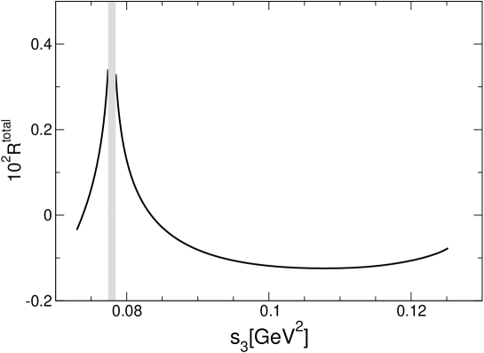
Figure 12: The ratio $R^{\rm{tot}}$ defined in Eq. (82), see text for more details. The grey band denotes the region Eq. (54), excluded in the data analysis of Ref. [9]. It is seen that the radiative corrections are very small in this case.

We display the resulting $R^{\rm{tot}}$ in Fig. 12 in the region defined in Eq. (54). We conclude from this figure that the radiative corrections to the amplitude are small in this channel.

7.4 On the soft-photon approximation

We wish to briefly discuss the quality of the soft-photon approximation of the bremsstrahlung calculation in the corrections factors $\Omega_{+-0}$ and $\Omega_{00+}$ as discussed in the previous two subsections.

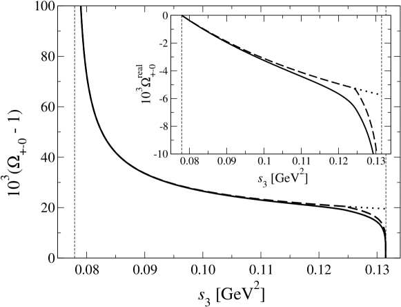
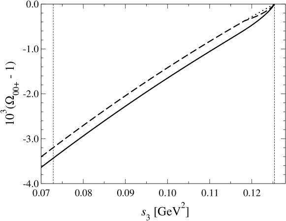
Figure 13: Comparison of the photon correction factors in the full calculation (solid lines) and the soft-photon approximation (dashed/dotted lines), for the channels $K_{L}\to\pi^{+}\pi^{-}\pi^{0}$ (upper panel) and $K^{+}\to\pi^{0}\pi^{0}\pi^{+}$ (lower panel), as functions of $s_{3}$. We have employed a photon cutoff energy of $E_{\mathrm{cut}}=10$ MeV. In the upper panel, the main plot shows $\Omega_{+-0}(s_{3},E^{n}_{\mathrm{max}})$ (in units of $10^{-3}$), while the insert represents $\Omega_{+-0}^{\rm real}(s_{3},E^{n}_{\mathrm{max}})\doteq\alpha/\pi\times\omega_{+-0}^{\rm real}(s_{3},E^{n}_{\mathrm{max}})$ alone, i.e. with the Coulomb pole subtracted. The lower panel shows $\Omega_{00+}(s_{3},E_{\mathrm{max}})$ (in units of $10^{-3}$). The vertical lines denote the allowed kinematical range in $s_{3}$. For more details, see main text.

In Fig. 13, these are plotted as functions of $s_{3}$ for a fixed photon cut energy $E_{\mathrm{cut}}=10$ MeV. Full lines denote the complete calculation, dashed lines the soft-photon approximation. In addition, the dotted lines show a “naive” soft-photon approximation with $E_{\mathrm{max}}=E_{\mathrm{cut}}$, i.e. one disregards the fact that the maximum photon energy is, in some parts of phase space, not given by $E_{\mathrm{cut}}$, but by the kinematical limit $E_{\mathrm{kin}}(s_{3})$, see Eq. (A.8). In the other cases, the correction factors are not smooth at the point where $E_{\mathrm{kin}}(s_{3})=E_{\mathrm{cut}}$.

For the channel $K_{L}\to\pi^{+}\pi^{-}\pi^{0}$, we find that, as power counting suggests, the Coulomb pole term in $\omega_{+-0}^{\rm virt}(s_{3})$ completely dominates $\Omega_{+-0}$. In the insert of the upper panel of Fig. 13, this term has therefore been subtracted to make the differences between the various curves more visible. Even so, we find that the soft-photon approximation is a very small effect, and the difference in $\Omega_{+-0}$ stays well below $2\times 10^{-3}$. However, there is a more significant deviation from the “naive” soft-photon approximation due to a logarithmic divergence at the upper kinematical limit for $s_{3}$, signalling that very close to the boundary of phase space, the approximation of $\mathcal{O}(\alpha)$ becomes unreliable.

For the channel $K^{+}\to\pi^{0}\pi^{0}\pi^{+}$, the correction factor is very small throughout phase space ($|1-\Omega_{00+}|<4\times 10^{-3}$), and the deviation due to the soft-photon approximation is smaller than $0.2\times 10^{-3}$. Furthermore, except for the region where the maximum photon energy is restricted by phase space, the correction factor is very close to linear and could therefore be largely absorbed in a coupling constant shift of the polynomial part of the amplitude.

We therefore confirm for both these $K\to 3\pi$ decay channels that a treatment of the bremsstrahlung corrections in the soft-photon approximation leads to negligible modifications in the pertinent correction factors.

7.5 $K^{+}\to\pi^{+}\pi^{+}\pi^{-}$

As the corrections to the soft-photon approximation for both $K_{L}\to\pi^{+}\pi^{-}\pi^{0}$ and $K^{+}\to\pi^{+}\pi^{0}\pi^{0}$ turn out to be negligible, we confine ourselves to this approximation for the last channel $K^{+}\to\pi^{+}\pi^{+}\pi^{-}$. In this case, the universal radiative corrections cannot be formulated as a function of the single variable $s_{3}$ any more, therefore we here define $\Omega_{++-}(s_{1},s_{2},s_{3},E_{\mathrm{max}})$ in terms of the differential decay width instead of the decay spectrum,

$$d\Gamma\bigr{|}_{E_{\gamma}<E_{\mathrm{max}}} =\Omega_{++-}(s_{1},s_{2},s_{3},E_{\mathrm{max}})d\Gamma^{\rm int}~{},$$ (83)

$$\Omega_{++-}(s_{1},s_{2},s_{3},E_{\mathrm{max}}) =1+\frac{\alpha}{\pi}\Bigl{(}\omega_{++-}^{\rm virt}(s_{1},s_{2},s_{3})+\omega_{++-}^{\rm real}(s_{3},E_{\mathrm{max}})\Bigr{)}+\mathcal{O}(\alpha^{2})~{}.$$

We remark briefly that the definition Eq. (83) (in contrast to Eqs. (66), (75)) is only unambiguous as long as the soft-photon approximation is applied, which neglects the photon in overall momentum conservation. Otherwise the allowed kinematic range for, say, $s_{1}$ and $s_{3}$ is different for the radiative process as compared to the non-radiative one.

All diagrams shown in Fig. 4a–f contribute for this channel, and we find the following result for virtual-photon corrections:

$$\mathrm{Re}\mathcal{M}_{++-}=\bigl{\{}H_{0}+H_{1}(p_{3}^{0}-M_{\pi})\bigr{\}}\biggl{[}1+e^{2}\biggl{(}\frac{1+\sigma_{1}^{2}}{16\sigma_{1}}+\frac{1+\sigma_{2}^{2}}{16\sigma_{2}}-\frac{1+\sigma_{3}^{2}}{16\sigma_{3}}\biggr{)}\biggr{]}\,,$$ (84)

where we use the notation $\sigma_{i}=\sqrt{1-4M_{\pi}^{2}/s_{i}}$. This results in

$$\omega_{++-}^{\rm virt}(s_{1},s_{2},s_{3})=\frac{\pi^{2}}{2}\biggl{[}\frac{1+\sigma_{1}^{2}}{\sigma_{1}}+\frac{1+\sigma_{2}^{2}}{\sigma_{2}}-\frac{1+\sigma_{3}^{2}}{\sigma_{3}}\biggr{]}~{}.$$ (85)

The soft-photon radiation contributions are calculated from the squared matrix element

$$|\mathcal{M}_{++-}^{\gamma}|^{2}=-e^{2}H_{0}^{2}\sum_{i,j=0}^{3}Q_{i}Q_{j}\frac{p_{i}p_{j}}{(p_{i}k)(p_{j}k)}~{},$$ (86)

where we use $p_{0}=P$ and the charges $Q_{0}=Q_{3}=-1$, $Q_{1}=Q_{2}=1$ for compactness. The significantly simpler calculation results in

$$\omega_{++-}^{\rm real}(s_{3},E_{\mathrm{max}}) =\frac{2\lambda_{c}}{3M_{K}^{2}M_{\pi}^{2}}\Bigl{(}\ln\frac{2E_{\mathrm{max}}}{M_{\pi}}-\frac{1}{3}\Bigr{)}+\mathcal{O}(\epsilon^{4},E_{\mathrm{max}})~{}.$$ (87)

The term $+\mathcal{O}(E_{\mathrm{max}})$ indicates once more that, in contrast to earlier sections, real photon emission is only treated in the soft-photon approximation.

As for the other supplementary channel $K_{L}\to\pi^{+}\pi^{-}\pi^{0}$, we disregard radiative corrections of order $e^{2}a^{1}$, therefore the amplitude $\mathcal{M}_{++-}^{\rm int}$ is given directly in terms of the amplitude $\mathcal{M}_{++-}$ in Ref. [6, 31, 45].

8 On the accuracy of a determination of $a_{0}-a_{2}$

In this section, we discuss the various sources of theoretical uncertainties that limit the accuracy of an experimental determination of $a_{0}-a_{2}$ from an analysis of the cusp in $K\to 3\pi$. For definiteness, we concentrate on the charged kaon decay channel $K^{+}\to\pi^{0}\pi^{0}\pi^{+}$. The authors of Ref. [4] were the first to quote a theoretical uncertainty on $a_{0}-a_{2}$, attributed to higher-order (three-loop) terms in the expansion in $a$ as well as radiative corrections. A simple order-of-magnitude estimate of terms of $\mathcal{O}(a^{3})$ led to a combined uncertainty of 5%. This assessment was roughly confirmed in Ref. [5], where the uncertainty is quoted as 5–7%.

The analytic structure of the various $K\to 3\pi$ amplitudes is now rather well understood, and combining the results of Refs. [6, 7] with the present investigation, one obtains a very accurate representation. We identify the following main sources of theoretical uncertainty, in partial agreement with Refs. [4, 5].

1. Electromagnetic corrections.

2. Isospin-breaking corrections in the matching of the coupling constants $C_{i}$ to the $\pi\pi$ scattering lengths.

3. Terms of order $a^{2}\epsilon^{4}$.

4. Higher-order loop corrections in the strong sector, starting at $\mathcal{O}(a^{3}\epsilon^{3})$ in the non-relativistic power counting.

Concerning point 1, we believe that the results presented in this article leave no significant error due to missing radiative corrections. This clearly is the main progress compared to earlier investigations. Concerning point 2, we have shown in Sect. 3.2 that the uncertainties are of the order of one percent. Examples of terms at $\mathcal{O}(a^{2}\epsilon^{4})$ mentioned in point 3 can be worked out by comparing the exact form of the two-loop integral $F$ in Eq. (13) with the explicit expressions at order $\epsilon^{2}$, provided in Ref. [7], or by partially adding effective range interaction vertices to the two-loop diagrams.

Finally, for an estimate of the uncertainty in point 4, we consider the threshold theorem [2, 3, 6] for $K^{+}\to\pi^{0}\pi^{0}\pi^{+}$ in the absence of photons: the leading non-analytic piece $\propto\sigma$ at the $\pi^{+}\pi^{-}$ threshold is given by the product of the decay amplitude $K^{+}\to\pi^{+}\pi^{+}\pi^{-}$ and the scattering amplitude $\pi^{+}\pi^{-}\to\pi^{0}\pi^{0}$, both evaluated at threshold. In particular, the coefficient of the cusp $\propto\sigma$ is proportional to

$$Z=T(K^{+}\to\pi^{+}\pi^{+}\pi^{-})\bigl{|}_{s_{1}=4M_{\pi}^{2},\,s_{2}=s_{3}=\frac{1}{2}(M_{K}^{2}-M_{\pi}^{2})}~{}.$$ (88)

A calculation of the quantity $Z$ to $\mathcal{O}(a^{n})$ therefore yields the strength of the leading cusp behavior as given in a representation of the decay amplitude $K^{+}\to\pi^{0}\pi^{0}\pi^{+}$ at $\mathcal{O}(a^{n+1})$, in other words, the two-loop representation of the $K^{+}\to\pi^{+}\pi^{+}\pi^{-}$ amplitude given in Ref. [6, 31, 45] allows for an estimate of $a^{3}$ effects on the cusp. Numerically, the expansion of $Z$ up to two loops reads in arbitrary normalization

$$Z\,=\,-1.0\,(\textrm{tree})\,-\,0.13\,i\,(\textrm{1-loop})\,+\,0.014\,(\textrm{2-loop})~{},$$ (89)

i.e. terms of order $a^{3}$ will modify the strength of the leading (one-loop) cusp by about 1.5%. The present estimate does not replace a full calculation of $\mathcal{O}(a^{3})$ effects, as it is necessarily incomplete: it neither yields a correct representation of the amplitude elsewhere in the Dalitz plot (except in the cusp region), nor does it give any information about subleading cusp behavior (e.g. $\propto\sigma^{3}$). However, we regard Eq. (89) as a good indication for the rate of convergence in the $K^{+}\to\pi^{0}\pi^{0}\pi^{+}$ amplitude and the error in the latter due to the omission of (strong) three-loop effects.

We may conclude from the above that the decay amplitude for $K^{+}\to\pi^{0}\pi^{0}\pi^{+}$ is indeed known very accurately. However, the accuracy to which the amplitude is known does not necessarily translate directly into the accuracy with which $a_{0}-a_{2}$ can be extracted from data. Rather, the latter is related to the change in the derivative of the amplitude (or the decay spectrum) in the vicinity of the cusp. We illustrate this point with the help of the loop function $J_{+-C}(s_{3})$, see Eq. (60), which is responsible for the “internal” radiative corrections in $K^{+}\to\pi^{0}\pi^{0}\pi^{+}$. Below $\pi^{+}\pi^{-}$ threshold, the singular part of it is given by

$$-\frac{1}{16\pi}\bigl{(}\tilde{\sigma}+\alpha\log\tilde{\sigma}\bigr{)}~{},\quad\tilde{\sigma}=\sqrt{\frac{4M_{\pi}^{2}}{s_{3}}-1}~{}.$$ (90)

The derivative with respect to $s_{3}$ slightly below threshold is given by

$$\frac{d}{ds_{3}}\biggl{[}-\frac{1}{16\pi}\bigl{(}\tilde{\sigma}+\alpha\log\tilde{\sigma}\bigr{)}\biggr{]}_{s_{3}=4M_{\pi}^{2}-\Delta}=\frac{1}{64\pi M_{\pi}\sqrt{\Delta}}\biggl{(}1+\frac{2\alpha M_{\pi}}{\sqrt{\Delta}}\biggr{)}+\ldots~{},$$ (91)

where higher-order terms in $\Delta/M_{\pi}^{2}$ have been neglected. So while the term of $\mathcal{O}(\alpha)$ may represent a very small correction on the absolute value of the amplitude, it changes the slope near the cusp, given by $J_{+-C}$ on a smooth (polynomial) background, by a relative factor of $2\alpha M_{\pi}/\sqrt{\Delta}$ that diverges near threshold. For example, at the lower bound of the exclusion region in the NA48/2 experimental analysis [9], $\Delta=\Delta_{s}=5.25\times 10^{-4}\,\mbox{GeV}^{2}$ (see Sect. 6), this relative factor is as large as 9%.

We do not doubt that a more reliable estimate of the theoretical uncertainty in $a_{0}-a_{2}$ is feasible by working it out along with the data analysis. As all the ingredients are available now, it would be useful to e.g. i) study the stability of $a_{0}-a_{2}$ with respect to changes in the choice of the exclusion region $\Delta_{s}$, as illustrated by the example above; ii) work out the influence of $a^{2}\epsilon^{4}$ terms as described above; iii) investigate the effect of Coulomb corrections at one vs. two-loop order.

9 Comparison with other work

Isidori [25] has considered the universal soft-photon corrections in multi-body meson decays and applied this specifically to the decay channel $K^{+}\to\pi^{+}\pi^{+}\pi^{-}$. The results for the virtual photon corrections correspond to a relativistic calculation, as it is discussed in Appendix D, i.e. they agree with our non-relativistic results up to polynomial terms (that can be absorbed in a redefinition of the polynomial part of the decay amplitude) and up to higher orders in the expansion in $\epsilon$. Note that these higher-order terms in $\epsilon$ are not complete in the sense that there are non-universal corrections of the same order (some of which have been discussed as neglected higher-order diagrams in Sect. 5). The real photon radiation corrections are considered in the soft-photon approximation, the effects of which we have discussed in Sect. 7.4. Our results agree with those given in Ref. [25] (up to typos) when expanding once more in $\epsilon$. Finally, Isidori [25] mentions the formation of Coulomb bound states (such as pionium) as one of the potentially relevant omissions in its discussion of radiative corrections. We have closed this gap here in Sect. 6.

In recent papers [26, 27] the isospin-breaking corrections to $K^{\pm}$ decays into three pions have been studied in a combined approach, where the treatment of the cusps resembles that in the non-relativistic effective field theory (see Refs. [6, 7] and the present work), whereas the electromagnetic effects are included within a quantum-mechanical approach. The treatment is not systematic. For example, in the strong sector the expression for the decay amplitude in our language corresponds to the summation of the one-loop pion loops with non-derivative couplings only. This expression has not been derived in Refs. [26, 27] and, as follows from the present work, can be valid only in the vicinity of the cusp and only up to and including $\mathcal{O}(\epsilon)$. The generalization to higher orders and beyond the cusp region is not discussed. The electromagnetic effects include the multi-Coulomb exchange within the charged pion loop that corresponds roughly to our Eq. (55). The procedure is again not systematic: Bremsstrahlung corrections, infrared divergences, etc. are not discussed. We therefore conclude that the results of Refs. [26, 27] cannot be safely used for the analysis of the experimental data on $K\to 3\pi$ decays.

The calculations of radiative corrections to $K\to 3\pi$ decays in Refs. [22, 23, 24] are performed in the framework of Chiral Perturbation Theory. Such a framework is not suited to an extraction of the $\pi\pi$ scattering lengths from experimental data, as these do not appear directly as parameters of the theory. Furthermore, the effects corresponding to our corrections of $\mathcal{O}(e^{2}a)$ that modify the analytic structure of the cusp are beyond the accuracy considered in Refs. [22, 23, 24] and are not considered there.

10 Summary and conclusions

In this article, we have generalized the framework of non-relativistic effective field theory for the cusp analysis in $K\to 3\pi$ decays to include real and virtual photon effects. This framework now allows one to calculate the relevant amplitudes systematically in a three-fold expansion in the non-relativistic expansion parameter $\epsilon$, $\pi\pi$ scattering lengths $a$, and the electromagnetic coupling $e^{2}$. We have performed this calculation up to $\mathcal{O}(e^{2}a^{0}\epsilon^{4})$ for all four $K\to 3\pi$ channels, and up to $\mathcal{O}(e^{2}a^{1}\epsilon^{2})$ for those channels in which the cusp effect is seen, namely $K^{+}\to\pi^{0}\pi^{0}\pi^{+}$ and $K_{L}\to 3\pi^{0}$. We have made consistency checks with the corresponding relativistic calculations of radiative corrections in various ways. Real bremsstrahlung has been calculated without the soft-photon approximation for $K^{+}\to\pi^{0}\pi^{0}\pi^{+}$ and $K_{L}\to\pi^{+}\pi^{-}\pi^{0}$, and the effect of this approximation could explicitly be shown to be small. The non-relativistic power counting provides a natural explanation for the common assumption that radiative corrections are dominated by Coulomb photon exchange, and that e.g. bremsstrahlung effects are very small. As an important phenomenon beyond the universal radiative corrections, we have studied the impact of pionium on the threshold (cusp) region.

We have provided simple analytic formulae for universal multiplicative correction factors on decay spectra or differential decay widths, and for modified decay amplitudes taking into account “internal” photon exchange processes. We have commented on the various issues concerning the theoretical uncertainties in the extraction of $a_{0}-a_{2}$ from the cusp effect. We expect that using this formalism in a refined analysis of the experimental data will lead to a precise determination of the $\pi\pi$ scattering lengths from $K\to 3\pi$ decays.

Acknowledgments

We would like to thank the members of NA48/2 for many useful discussions and a very fruitful collaboration, in particular Brigitte Bloch-Devaux, Luigi Di Lella, Dmitry Madigozhin, and Italo Mannelli. In particluar, we thank Luigi Di Lella and Dmitry Madigozhin for performing specific fits to $K\to 3\pi$ data with our amplitudes. Furthermore, discussions with Sergey R. Gevorkyan and Slawomir Wycech as well as useful e-mail exchanges with Gino Isidori are gratefully acknowledged. Partial financial support under the EU Integrated Infrastructure Initiative Hadron Physics Project (contract number RII3–CT–2004–506078) and DFG (SFB/TR 16, “Subnuclear Structure of Matter”) is gratefully acknowledged. This work was supported by the Swiss National Science Foundation, by EU MRTN–CT–2006–035482 (FLAVIAnet), and by the Helmholtz Association through funds provided to the virtual institute “Spin and strong QCD” (VH-VI-231). One of us (J.G.) is grateful to the Alexander von Humboldt–Stiftung and to the Helmholtz–Gemeinschaft for the award of a prize that allowed him to stay at the HISKP at the University of Bonn, where part of this work was performed. He also thanks the HISKP for the warm hospitality during these stays.

Appendix A Notation, kinematics

In this appendix, we briefly collect some of the notation that is used throughout the article. The masses of the charged pions are denoted by $M_{\pi}$ while for the neutral pion, $M_{\pi^{0}}$ is used. Accordingly, $M_{K}$ denotes the charged kaon mass and $M_{K_{\!L}}$ that of the $K_{L}$. The decay channels are abbreviated by indicating the charge of the final state pions, and the momenta are assigned in the usual convention such that the odd pion carries four momentum $p_{3}$.

decay channel	abbreviation
$K_{L}(P)\to\pi^{0}(p_{1})\pi^{0}(p_{2})\pi^{0}(p_{3})$	$(0,0,0)$
$K_{L}(P)\to\pi^{+}(p_{1})\pi^{-}(p_{2})\pi^{0}(p_{3})$	$(+,-,0)$
$K^{+}(P)\to\pi^{0}(p_{1})\pi^{0}(p_{2})\pi^{+}(p_{3})$	$(0,0,+)$
$K^{+}(P)\to\pi^{+}(p_{1})\pi^{+}(p_{2})\pi^{-}(p_{3})$	$(+,+,-)$

The Mandelstam variables are defined as

$$s_{1}=(p_{2}+p_{3})^{2}\,,\quad\mbox{cycl.}$$ (A.1)

In the charged kaon rest frame, the energy and 3-momentum of the pions are given by

$$p_{i}^{0}=\frac{M_{K}^{2}+M_{i}^{2}-s_{i}}{2M_{K}}\,,\qquad{\bf p}_{i}^{2}=\frac{\lambda(M_{K}^{2},M_{i}^{2},s_{i})}{4M_{K}^{2}}$$ (A.2)

(in the neutral kaon decays $M_{K}\to M_{K_{\!L}}$). In the above equation, we have used

$$\lambda(x,y,z) =x^{2}+y^{2}+z^{2}-2xy-2xz-2yz\,.$$ (A.3)

Furthermore, the following functions of kinematical variables are frequently used:

$$\lambda_{0} =\lambda\left(M_{K_{\!L}}^{2},s_{3},M_{\pi^{0}}^{2}\right)\,, \lambda_{c} =\lambda\left(M_{K}^{2},s_{3},M_{\pi}^{2}\right)\,,$$

$$\sigma =\sqrt{1-\frac{4M_{\pi}^{2}}{s_{3}}}\,, q_{0}^{2} =\frac{s_{3}}{4}-M_{\pi}^{2}=\frac{s_{3}\,\sigma^{2}}{4}\,.$$ (A.4)

The maximum photon energy $E_{\mathrm{max}}$ ($E^{n}_{\mathrm{max}}$) for $K^{+}$ ($K_{L}$) decays in the kaon rest frame is given by

$$E_{\mathrm{max}}^{(n)} =\left\{\begin{array}[]{c@{\quad: \quad}l}E_{\mathrm{kin}}^{(n)}&E_{\mathrm{kin}}^{(n)}<E_{\mathrm{cut}}\\ E_{\mathrm{cut}}&E_{\mathrm{kin}}^{(n)}>E_{\mathrm{cut}}\end{array}\right.~{},\qquad\textrm{where}$$ (A.7)

$$E_{\mathrm{kin}} =\frac{M_{K}^{2}-(M_{\pi}+\sqrt{s_{3}})^{2}}{2M_{K}}~{},\quad E_{\mathrm{kin}}^{n}=\frac{M_{K_{\!L}}^{2}-(M_{\pi^{0}}+\sqrt{s_{3}})^{2}}{2M_{K_{\!L}}}\,.$$ (A.8)

Loop integrations are denoted by an angle bracket and the pole in four dimensions is contained in the term $\lambda$,

$$\left\langle\ldots\right> =\int\frac{d^{D}l}{i(2\pi)^{D}}\ldots\,, D =d+1\,,$$

$$\lambda =\frac{\mu^{D-4}}{16\pi^{2}}\left[\frac{1}{D-4}-\frac{1}{2}\left(\Gamma^{\prime}(1)+\ln(4\pi)+1\right)\right]\,.$$ (A.9)

In the text, we also use – depending on the context – the symbols $\lambda_{IR}$ or $\lambda_{UV}$ for this quantity.

The differential decay width for the $n$-body decay of a particle of mass $M$ in $D=4$ dimensions is given in terms of the matrix element $\mathcal{M}$ according to

$$d\Gamma =Nd\Phi_{n}(P;p_{1},\ldots,p_{n})|\mathcal{M}|^{2}~{},$$

$$N =\frac{(2\pi)^{4}}{2M}\frac{1}{S}~{},\quad d\Phi_{n}(P;p_{1},\ldots,p_{n})=\delta^{4}\Bigl{(}P-\sum_{i=1}^{n}p_{i}\Bigr{)}\prod_{i=1}^{n}\frac{d^{3}p_{i}}{2p_{i}^{0}(2\pi)^{3}}~{}.$$ (A.10)

where the values of the symmetry factor and the mass, $(S,M)$, are $(2,M_{K})$ for $(0,0,+)$ and $(+,+,-)$, $(1,M_{K_{\!L}})$ for $(+,-,0)$ and $(6,M_{K_{\!L}})$ for $(0,0,0)$. For the phase space integrations in $D=d+1\neq 4$ dimensions, we generalize Eq. (A.10) using

$$N(d)=\frac{(2\pi)^{D}}{2M}\frac{1}{S}\,,\quad d\mu(p)=\frac{d^{d}p}{2p^{0}(2\pi)^{d}}\,,\quad\Omega_{d}=\frac{2\pi^{\frac{d+1}{2}}}{\Gamma(\frac{d+1}{2})}\,,$$

$$d\Phi_{n}(P;p_{1},\ldots,p_{n},d)=\delta^{D}\Bigl{(}P-\sum_{i=1}^{n}p_{i}\Bigr{)}\prod_{i=1}^{n}d\mu(p_{i})~{}.$$ (A.11)

The cut of the logarithm is chosen, as usual, on the negative real axis and the $\psi$ function and the dilogarithm are defined as

$$\psi(x) =\frac{d}{dx}\ln\Gamma(x)\,, \mbox{Li}_{2}(z) =-\int_{0}^{1}dx\,\frac{\ln(1-xz)}{x}\,.$$ (A.12)

Appendix B Radiative corrections: relativistic framework

The non-relativistic calculation presented in the main text is quite complex. In order to have a fully independent check on that calculation, in this appendix we evaluate radiative corrections in a relativistic framework, for the two decay channels $(+,-,0)$ and $(0,0,+)$. In particular, we work out the corrections $\Omega_{+-0}$ and $\Omega_{00+}$ (see Eqs. (66), (75)) in the relativistic framework and compare the result with the non-relativistic calculation described in the main text. We confirm that, to the order considered in the momentum expansion, the relativistic result indeed is identical to the non-relativistic one, up to a redefinition of tree-level couplings. Note that, as the purpose of this Appendix is mainly to cross-check the non-relativistic calculation, we also here disregard all one-photon and one-pion reducible graphs (see e.g. Ref. [23]), which turn into polynomial terms when expanded non-relativistically in $\epsilon$.

In the present Appendix, the final results of this calculation are presented. The pertinent contributions include virtual and real photons. The evaluation of Bremsstrahlung is performed in Appendix C, whereas the relativistic loop integrals are detailed in Appendix D.

The calculation is performed in the Feynman-gauge. Infrared and ultraviolet divergences are both tamed with dimensional regularization. In keeping with the standard procedure for calculations of radiative corrections in a relativistic framework, we retain the distinction between both types of divergences in this appendix. To make the formulae more transparent, we use the same scale for both, UV and IR divergences, although the origin of the divergences can be clearly identified. We therefore use the notation

$$\lambda_{UV}=\frac{\mu^{D-4}}{16\pi^{2}}\left[\frac{1}{D-4}-\frac{1}{2}\left(\Gamma^{\prime}(1)+\ln(4\pi)+1\right)\right]=\lambda_{IR}\,.$$ (B.1)

The loop integrals $\Lambda_{+},\Lambda_{0},T_{i}^{ab},\bar{J}^{ab}$ may be found in Appendix D, and the Bremsstrahlung integrals $I_{i}^{f}$ are given in Appendix C, together with the symbols $\delta_{0,c}$. As already mentioned in the main text, we evaluate real photon emission beyond the soft-photon approximation.

B.1 $K^{+}\to\pi^{0}\pi^{0}\pi^{+}$

We first consider the decay $K^{+}(P)\to\pi^{0}(p_{1})\pi^{0}(p_{2})\pi^{+}(p_{3})$. The relativistic interaction Lagrangian is

$$\mathcal{L}_{\rm int} = \frac{G_{0}}{2}(1+e^{2}b)(K^{\dagger}\pi\pi^{0}\pi^{0}+\mathrm{h.c.})\,\,,$$

$$b = 6\lambda_{UV}+b_{r}(\mu)\,\,.$$ (B.2)

Here and in the following, we do not explicitly write the couplings to photons, because these are trivially constructed via minimal coupling.

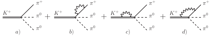
Figure B.1: Virtual photon corrections to the $K^{+}\to\pi^{0}\pi^{0}\pi^{+}$ decay.

The virtual corrections displayed in Fig. B.1 generate the contribution

$$\mathcal{M}^{\mathrm{virt}}(s_{3})=G_{0}\left[Z-e^{2}\Lambda_{+}(s_{3})\right]\,;\,s_{3}=(P-p_{3})^{2}\,\,.$$

The $Z$-factor is

$$Z=1-4e^{2}\left(\lambda_{UV}-\lambda_{IR}\right)\,.$$ (B.3)

Since the amplitude depends only on $s_{3}$, integration over phase space gives for the decay spectrum in $d$ dimensions

$$\frac{d\Gamma}{ds_{3}} = N(d)(2\pi)^{d}\Phi_{2}(M_{K}^{2},s_{3},m_{3}^{2},d)\Phi_{2}(s_{3},m_{1}^{2},m_{2}^{2},d)|\mathcal{M}^{\mathrm{virt}}(s_{3})|^{2}\,,$$ (B.4)

where $\Phi_{2}$ denotes the two-particle phase space in $d$ dimensions, see Eq. (C.6), and where $p_{i}^{2}=m_{i}^{2}$. We add Bremsstrahlung contributions, worked out in Appendix C. These cancel the infrared divergences generated by $\cal{M}^{\mathrm{virt}}$. Finally, we determine the relativistic analogon of the correction factor introduced in Eq. (75). Using the notation $\Omega_{00+}\to\Omega^{R}_{00+}$, we find

$$\Omega^{R}_{00+}(s_{3},E_{\mathrm{max}}) =1+\frac{\alpha}{\pi}[F_{1}+F_{2}+F_{3}]+\mathcal{O}(\alpha^{2})\,,$$ (B.5)

$$F_{1} =A\,\left(L_{E}\,T_{1}^{K\pi}(s_{3})-T_{2}^{K\pi}(s_{3})\right)\,,$$

$$F_{2} =\frac{M_{K}^{2}}{\sqrt{\lambda_{c}}}\left[2I_{4}^{f}(s_{3},E_{\mathrm{max}})-I_{2}^{f}(s_{3},E_{\mathrm{max}})-I_{3}^{f}(s_{3},E_{\mathrm{max}})\right]\,,$$

$$F_{3} =8\pi^{2}b_{r}(\mu)-3\ln\frac{M_{\pi}}{\mu}-2L_{E}+\frac{M_{\pi}^{2}}{M_{K}^{2}-M_{\pi}^{2}}\ln\frac{M_{K}}{M_{\pi}}-8\pi^{2}\bar{J}^{K\pi}(s_{3})\,,$$

where

$$L_{E}=\ln\left(\frac{2E_{\mathrm{max}}M_{K}}{\sqrt{\lambda_{c}}}\right)\,,\,\,\,A=\frac{M_{K}^{2}+M_{\pi}^{2}-s_{3}}{M_{\pi}^{2}}\,.$$ (B.6)

To compare with $\Omega_{00+}$, we expand $\Omega^{R}_{00+}$ in $\epsilon$ up to and including $\mathcal{O}(\epsilon^{3})$,

$$\Omega^{R}_{00+}(s_{3},E_{\mathrm{max}}) =1+\frac{\alpha}{\pi}\biggl{\{}8\pi^{2}b_{r}(\mu)-3\ln\frac{M_{\pi}}{\mu}-\frac{5}{2}+\frac{3}{2}\Bigl{(}1-\frac{M_{K}\!-\!3M_{\pi}}{2M_{\pi}}\Bigr{)}\ln\frac{M_{K}}{M_{\pi}}$$

$$+\frac{\lambda_{c}}{6M_{K}^{2}M_{\pi}^{2}}\biggl{[}\ln\frac{2E_{\mathrm{max}}}{M_{\pi}}-\frac{97}{24}+\frac{19}{8}\ln 3+\frac{2}{3}\Bigl{(}(4-\delta_{c})\sqrt{1-\delta_{c}}-4\Bigr{)}$$

$$\qquad\qquad-2\ln\frac{1+\sqrt{1-\delta_{c}}}{2}\biggr{]}+\mathcal{O}(\epsilon^{4})\biggr{\}}+\mathcal{O}(\alpha^{2})\,.$$ (B.7)

It is seen that $\Omega^{R}_{00+}$ differs from $\Omega_{00+}$ by a polynomial in the external momenta, which can be eliminated by a redefinition of the tree-level coupling constants. We conclude that the relativistic calculation confirms the non-relativistic result for $\Omega_{00+}$ presented in the main text.

B.2 $K_{L}\to\pi^{+}\pi^{-}\pi^{0}$

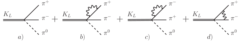
Figure B.2: Virtual photon corrections to the $K_{L}\to\pi^{+}\pi^{-}\pi^{0}$ decay.

Here we consider the decay $K_{L}(P)\to\pi^{+}(p_{1})\pi^{-}(p_{2})\pi^{0}(p_{3})$. The relativistic interaction Lagrangian is

$$\mathcal{L}_{\rm int} = L_{0}(1+e^{2}a)K_{L}\pi^{0}\pi^{\dagger}\pi\,,$$

$$a = 6\lambda_{UV}+a_{r}(\mu)\,.$$ (B.8)

The graphs displayed in Fig. B.2 generate the amplitude

$$\mathcal{M}^{\mathrm{virt}}(s_{3}) = L_{0}\left[Z+e^{2}\Lambda_{0}(s_{3})\right]\,;\,s_{3}=(P-p_{3})^{2}\,.$$ (B.9)

The $Z$-factor was already given in Eq. (B.3). We use the analogue of Eq. (B.4), and combine the result with real photon emission considered in Appendix C. The relativistic correction factor $\Omega^{R}_{+-0}$, the analogue of $\Omega_{+-0}$ in Eq. (66), becomes

$$\Omega^{R}_{+-0}(s_{3},E^{n}_{\mathrm{max}}) =1+\frac{\alpha}{\pi}\left(f_{1}+f_{2}+f_{3}\right)+\mathcal{O}(\alpha^{2})\,,$$

$$f_{1} =2B\,\left(\mbox{Re}\,T_{2}^{\pi\pi}(s_{3})-\Big{[}1+L^{n}_{E}+\frac{1}{1+\sigma^{2}}\Big{]}\mbox{Re}\,T_{1}^{\pi\pi}(s_{3})\right)\,,$$

$$f_{2} =-\frac{2M_{K_{\!L}}^{2}s_{3}}{\sqrt{\lambda_{0}}M_{\pi}^{2}}\,\bigl{[}B\,\mbox{Re}\,T_{1}^{\pi\pi}(s_{3})+1\bigr{]}I_{1}^{f}(s_{3},E^{n}_{\mathrm{max}})\,,$$

$$f_{3} =-\frac{5}{2}+8\pi^{2}a_{r}(\mu)-3\ln\frac{M_{\pi}}{\mu}-2L^{n}_{E}+\frac{\sigma}{2}\ln\Bigl{(}\frac{1+\sigma}{1-\sigma}\Bigr{)}$$

$$\quad+\frac{1+\sigma^{2}}{2\sigma}\left[\mbox{Li}_{2}\Bigl{(}\frac{2\sigma}{\sigma-1}\Bigr{)}-\mbox{Li}_{2}\Bigl{(}\frac{2\sigma}{\sigma+1}\Bigr{)}\right]\,,$$ (B.10)

where

$$L^{n}_{E} =\ln\left(\frac{2E^{n}_{\mathrm{max}}M_{K_{\!L}}}{\sqrt{\lambda_{0}}}\right)\,, B =\frac{1+\sigma^{2}}{1-\sigma^{2}}\,.$$ (B.11)

Expanding the result in $\epsilon$ up to and including $\mathcal{O}(\epsilon^{3})$, we obtain

$$\Omega^{R}_{+-0} =1+\frac{\alpha}{\pi}\Bigg{\{}\frac{\pi^{2}(1+\sigma^{2})}{2\sigma}+8\pi^{2}a_{r}(\mu)-3\ln\frac{M_{\pi}}{\mu}-\frac{5}{2}$$

$$\qquad+\frac{8\sigma^{2}}{3}\bigg{[}\ln\frac{2E^{n}_{\mathrm{max}}}{M_{\pi}}-\frac{85}{24}+2\sqrt{1-\delta_{0}}-2\ln\Bigl{(}\frac{1+\sqrt{1-\delta_{0}}}{2}\Bigr{)}\bigg{]}+\mathcal{O}(\epsilon^{4})\Bigg{\}}$$

$$\quad+\mathcal{O}(\alpha^{2})~{}.$$ (B.12)

This expression agrees with $\Omega_{+-0}$ in Eqs. (68), (71), (74) up to a polynomial in the external momenta, which can be absorbed with a redefinition of the tree-level couplings. We conclude that the relativistic calculation confirms the non-relativistic result for $\Omega_{+-0}$ presented in the main text.

Appendix C Bremsstrahlung beyond the soft-photon approximation

In this appendix, we evaluate the phase space integrals used in the calculations of the bremsstrahlung corrections to $K\to 3\pi$ decays, with a kinematical cut $E_{\mathrm{cut}}$ in the photon energy in the rest frame of the kaon. The evaluation of the decay spectra is, therefore, performed in this frame.

Most of the notation is set in Appendix A. In order to tame infrared singularities, we perform the phase space integrations in $d$ dimensions and indicate this with an additional argument $d$ in the infinitesimal $n$-body phase space element $d\Phi_{n}$. The differential decay width is defined as

$$d\Gamma=N(d)d\Phi_{4}(P;p_{1},p_{2},q,k,d)\left|\mathcal{M}\right|^{2}\,,$$ (C.1)

where $q$ and $k$ are the momenta of the odd pion and the photon, respectively. In a first step, the four particle phase space is separated in a three particle phase space integration over a two particle phase space integration,

$$\int d\Phi_{4}(P;p_{1},p_{2},q,k,d)=(2\pi)^{d}\!\int ds_{3}\,d\Phi_{2}(Q;p_{1},p_{2},d)d\Phi_{3}(P;Q,q,k,d)\,,$$

where $Q^{2}=s_{3}$.

C.1 $K^{+}\to\pi^{0}\pi^{0}\pi^{+}$

We illustrate the calculation with the simplest possible case $(0,0,+)$. The amplitude squared is given in Sect. 7.3. After performing the two particle phase space integration, the integration over $Q$ and over the angle between the photon and the charged pion as well as their angular parts, one is left with the integrations over the photon- and the $\pi^{+}$-energy. The boundaries of these integrations are given by

$$q^{0}_{\pm} =\frac{Y\pm k\sqrt{X}}{2M_{K}(M_{K}-2k)}\,, Y =(M_{K}-k)(M_{K}^{2}+M_{\pi}^{2}-s_{3}-2M_{K}k)\,,$$

$$X =\lambda_{c}+4kM_{K}\Delta_{+}\,,\!\! \Delta_{i} =s_{3}+M_{\pi^{i}}^{2}-M_{K}^{2}+M_{K}k\,,$$

$$E_{\mathrm{kin}} =\frac{M_{K}^{2}-(M_{\pi}+\sqrt{s_{3}})^{2}}{2M_{K}}\,, \!\!E_{\mathrm{max}} =\left\{\begin{array}[]{c@{\quad: \quad}l}E_{\mathrm{kin}}&E_{\mathrm{kin}}<E_{\mathrm{cut}}\\ E_{\mathrm{cut}}&E_{\mathrm{kin}}>E_{\mathrm{cut}}\end{array}\right.\,.$$ (C.4)

The integral reads

$$\frac{d\Gamma}{ds_{3}} = -G_{0}^{2}e^{2}(2\pi)^{d}N(d)\Phi_{2}(s_{3},M_{\pi^{0}}^{2},M_{\pi^{0}}^{2},d)\left[I_{2}+I_{3}-2I_{4}\right]\,,$$

$$I_{i} = \frac{\Omega_{d-2}\Omega_{d-1}}{8(2\pi)^{3d}}\int_{0}^{E_{\mathrm{max}}}dk\,k^{d-5}\int_{q^{0}_{-}}^{q^{0}_{+}}dq^{0}\,f_{i}(k,q^{0},d)\,,$$ (C.5)

where the two-particle phase space volume in $d$ dimensions is given by

$$\Phi_{2}(s,m_{1}^{2},m_{2}^{2},d)=\int d\Phi_{2}(P;p_{1},p_{2},d)=\frac{2}{(4\pi)^{\frac{3d}{2}}\Gamma(\frac{d}{2})\sqrt{s}}\bigg{(}\frac{\lambda(s,m_{1}^{2},m_{2}^{2})}{s}\bigg{)}^{\frac{d-2}{2}}$$ (C.6)

with $P^{2}=s$, $p_{i}^{2}=m_{i}^{2}\,,$ and

$$f_{2}(q^{0},k,d) =(q\sqrt{1-z^{2}})^{d-3}\,, f_{3}(q^{0},k,d) =M_{\pi}^{2}\frac{(q\sqrt{1-z^{2}})^{d-3}}{(q^{0}-qz)^{2}}\,,$$

$$f_{4}(q^{0},k,d) =q^{0}\frac{(q\sqrt{1-z^{2}})^{d-3}}{q^{0}-qz}\,, q =\sqrt{q_{0}^{2}-M_{\pi}^{2}}\,,$$

$$z=\frac{M_{K}^{2}+M_{\pi}^{2}-s_{3}+2(kq^{0}-M_{K}q^{0}-kM_{K})}{2kq}\,.$$

We carry out the calculation in quite some detail for the integral $I_{2}$, the other integrals can be performed along the same lines.

Introduce the variable $u$ as $q^{0}=\bar{q}^{0}+ku$

$$I_{2} = \frac{\Omega_{d-2}\Omega_{d-1}}{8(2\pi)^{3d}}\int_{0}^{E_{\mathrm{max}}}dk\,k^{d-4}\int_{u_{-}(k)}^{u_{+}(k)}du\,g(u,k)^{d-3}\,,$$ (C.7)

with the functions

$$\bar{q}^{0} =\frac{M_{K}^{2}+M_{\pi}^{2}-s_{3}}{2M_{K}}\,, \bar{q} =\frac{\sqrt{\lambda_{c}}}{2M_{K}}\,, u_{\pm}(k) =\frac{q^{0}_{\pm}-\bar{q}^{0}}{k}\,,$$

$$z =\frac{\bar{q}^{0}-M_{K}(1+u)+ku}{q}\,, g(u,k) =q\sqrt{1-z^{2}}\,.$$ (C.8)

To isolate the infrared singular part we split up the function $g$ in a part with photon momentum zero and a remainder,

$$g(u,k)^{d-3} = g(u,0)^{d-3}+\Delta g(u,k)\,,$$

$$\Delta g(u,k) = g(u,k)^{d-3}-g(u,0)^{d-3}$$ (C.9)

$$= (d-3)\ln\left(\frac{g(u,k)}{g(u,0)}\right)+\mathcal{O}\bigl{(}(d-3)^{2}\bigr{)}\,.$$

Since the photon momentum dependent function $\Delta g$ is proportional to $k^{\alpha}$ with $\alpha>0$, this integral vanishes in the limit $d\to 3$ and we can drop it. The phase space integral has an infrared divergence proportional to $(d-3)^{-1}$, therefore, in a next step, we expand the remaining function $g(u,0)^{d-3}$ in the vicinity of $d=3$ and keep only terms up to and including $\mathcal{O}(d-3)$. Therefore, the original integral reads

$$I_{2} =\frac{\Omega_{d-2}\Omega_{d-1}}{8(2\pi)^{3d}}M_{\pi}^{d-3}\int_{0}^{E_{\mathrm{max}}}\!dk\,k^{d-4}\left[G_{2}(k)+(d-3)H_{2}(k)+\mathcal{O}\bigl{(}(d-3)^{2}\bigr{)}\right]\,,$$

$$G_{2}(k) =u_{+}(k)-u_{-}(k)\,,\quad H_{2}(k)=\int_{u_{-}(k)}^{u_{+}(k)}du\,\ln\Bigl{(}\frac{g(u,0)}{M_{\pi}}\Bigr{)}\,.$$ (C.10)

Splitting up the functions $G_{2}(k)$ and $H_{2}(k)$ as well in a photon momentum dependent and independent part, the original integral can be written as

$$I_{2}=I_{2}^{IR}+\frac{1}{512\pi^{7}}I_{2}^{f}(s_{3},E_{\mathrm{max}})+\mathcal{O}(d-3)\,.$$ (C.11)

where

$$I_{2}^{IR} =G_{2}(0)\frac{\Omega_{d-2}\Omega_{d-1}}{8(2\pi)^{3d}}\biggl{(}\frac{E_{\mathrm{max}}M_{\pi}}{\mu^{2}}\biggr{)}^{d-3}\frac{\mu^{2(d-3)}}{d-3}\,,$$

$$I_{2}^{f}(s_{3},E_{\mathrm{max}}) =H_{2}(0)+\int_{0}^{E_{\mathrm{max}}}dk\frac{\Delta G_{2}(k)}{k}\,,$$

$$G_{2}(0) =\frac{\sqrt{\lambda_{c}}}{M_{K}^{2}}\,,\qquad H_{2}(0)=\frac{\sqrt{\lambda_{c}}}{M_{K}^{2}}\left[\ln\left(\frac{\sqrt{\lambda_{c}}}{M_{K}M_{\pi}}\right)-1\right]\,,$$

$$\frac{\Delta G_{2}(k)}{k} =\frac{1}{M_{K}^{2}(M_{K}-2k)}\left[\frac{4M_{K}^{2}\Delta_{+}}{\sqrt{\lambda_{c}+4M_{K}k\Delta_{+}}+\sqrt{\lambda_{c}}}+2\sqrt{\lambda_{c}}\right]\,.$$ (C.12)

The part $I_{2}^{IR}$ contains the infrared singularity of $I_{2}$ as well as finite terms. Therefore, the part $I_{2}^{f}$ can be evaluated in $d=3$. Applying the same procedure to the remaining integrals, they divide again into two parts,

$$I_{i}=I_{i}^{IR}+\frac{1}{512\pi^{7}}I_{i}^{f}(s_{3},E_{\mathrm{max}})+\mathcal{O}(d-3)\,,\quad i=3,4\,,$$ (C.13)

and one finds

$$I_{i}^{f}(s_{3},E_{\mathrm{max}}) =H_{i}(0)+\int_{0}^{E_{\mathrm{max}}}dk\frac{\Delta G_{i}(k)}{k}\,,$$

$$I_{3}^{IR} =I_{2}^{IR}\,,\qquad I_{4}^{IR}=G_{4}(0)\frac{\Omega_{d-2}\Omega_{d-1}}{8(2\pi)^{3d}}\left(\frac{E_{\mathrm{max}}M_{\pi}}{\mu^{2}}\right)^{d-3}\frac{\mu^{2(d-3)}}{d-3}\,,$$

where

$$\frac{\Delta G_{3}(k)}{k} =\frac{4\Delta_{+}}{M_{K}(\sqrt{\lambda_{c}+4M_{K}k\Delta_{+}}+\sqrt{\lambda_{c}})}\,,$$

$$\frac{\Delta G_{4}(k)}{k} =\frac{1}{M_{K}}\biggl{[}\frac{\bar{q}^{0}}{k}\ln\left(\frac{1+D_{+}}{1+D_{-}}\right)-\ln\left(\frac{1+u_{+}(k)}{1+u_{-}(k)}\right)+u_{+}(k)-u_{-}(k)\biggr{]}\,,$$

$$H_{3}(0) =\frac{\sqrt{\lambda_{c}}}{2M_{K}^{2}}\left[2\ln\left(\frac{\sqrt{\lambda_{c}}}{M_{K}M_{\pi}}\right)-\frac{\bar{q}^{0}}{\bar{q}}\ln\left(\frac{\bar{q}^{0}+\bar{q}}{\bar{q}^{0}-\bar{q}}\right)\right]\,,$$

$$H_{4}(0) =\frac{\bar{q}^{0}}{2M_{K}}\left[2\ln\left(\frac{\sqrt{\lambda_{c}}}{M_{K}M_{\pi}}\right)\ln\left(\frac{\bar{q}^{0}+\bar{q}}{\bar{q}^{0}-\bar{q}}\right)+\mathrm{Li}_{2}\left(\frac{2\bar{q}}{\bar{q}-\bar{q}^{0}}\right)-\mathrm{Li}_{2}\left(\frac{2\bar{q}}{\bar{q}+\bar{q}^{0}}\right)\right],$$

$$G_{4}(0) =\frac{\bar{q}^{0}}{M_{K}}\ln\left(\frac{1+u_{+}(0)}{1+u_{-}(0)}\right)\,,$$

$$D_{\pm} =\pm\frac{\sqrt{\lambda_{c}+4M_{K}k\Delta_{+}}-\sqrt{\lambda_{c}}\mp 2kM_{K}}{2M_{K}\bar{q}^{0}\pm\sqrt{\lambda_{c}}}\,.$$ (C.14)

The remaining integrations over $u$ and $k$ can be done numerically in three dimensions, as they are free of infrared divergences.

The bremsstrahlung decay spectrum can be simplified considerably by expanding the infrared finite part of the combination $I_{2}+I_{3}-2I_{4}$ that appears in Eq. (C.1) in the non-relativistic parameter $\epsilon$. We find

$$H_{2}(0) +H_{3}(0)-2H_{4}(0)~{}=~{}\frac{\lambda_{c}^{3/2}}{36M_{K}^{4}M_{\pi}^{2}}\biggl{(}5-6\ln\frac{\sqrt{\lambda_{c}}}{M_{K}M_{\pi}}\biggr{)}+\mathcal{O}(\epsilon^{5})\,,$$

$$\int_{0}^{E_{\mathrm{max}}}dk \frac{\Delta G_{2}(k)+\Delta G_{3}(k)-2\Delta G_{4}(k)}{k}$$

$$=\frac{\lambda_{c}^{3/2}}{9M_{K}^{4}M_{\pi}^{2}}\biggl{(}4-(4-\delta_{c})\sqrt{1-\delta_{c}}+3\ln\frac{1+\sqrt{1-\delta_{c}}}{2}\biggr{)}+\mathcal{O}(\epsilon^{5})\,,$$

$$\delta_{c} =\frac{8M_{K}(M_{K}-M_{\pi})M_{\pi}E_{\mathrm{max}}}{\lambda_{c}}\,.$$ (C.15)

C.2 $K_{L}\to\pi^{+}\pi^{-}\pi^{0}$

In the decay channel $(+,-,0)$, the four particle phase space is again separated in a three particle phase space integration over a two particle phase space integration. However, because the amplitude squared indicated in Sect. 7.2 depends on the momenta of the two particle phase space integration, this two particle phase space does not factorize anymore, but produces the functions $R_{1}$ and $R_{2}$,

$$\frac{d\Gamma}{ds_{3}} =-8L_{0}^{2}e^{2}N(d)\Omega_{d-2}\Phi_{2}(s_{3},M_{\pi}^{2},M_{\pi}^{2},d)\Gamma\left(\frac{d}{2}\right)\frac{(4\pi)^{\frac{d}{2}}}{1-\sigma^{2}}\left[R_{1}-\frac{1+\sigma^{2}}{2}R_{2}\right]I_{1}\,,$$

$$R_{1} =1+(d-3)\left(\ln 2-\frac{1}{2\sigma}L\right)\,,\qquad L=\ln\frac{1+\sigma}{1-\sigma}\,,$$

$$R_{2} =\frac{1}{\sigma}L+\frac{d-3}{2\sigma}\left(2\ln 2\,L+\mathrm{Li}_{2}\left(\frac{2\sigma}{\sigma-1}\right)-\mathrm{Li}_{2}\left(\frac{2\sigma}{\sigma+1}\right)\right)\,,$$ (C.16)

where $R_{1}$ and $R_{2}$ are evaluated in a vicinity of $d=3$ and the two particle phase space volume $\Phi_{2}$ is given in Eq. (C.6). The remaining three particle phase space integrals can be solved along the lines of the previous section, and one obtains

$$I_{1} = I_{1}^{IR}+\frac{1}{512\pi^{7}}I_{1}^{f}(s_{3},E^{n}_{\mathrm{max}})\,,$$

$$I_{1}^{IR} = G_{1}(0)\frac{\Omega_{d-2}\Omega_{d-1}}{8(2\pi)^{3d}}\left(\frac{E^{n}_{\mathrm{max}}M_{\pi}}{\mu^{2}}\right)^{d-3}\frac{\mu^{2(d-3)}}{d-3}\,,$$

$$I_{1}^{f}(s_{3},E^{n}_{\mathrm{max}}) = H_{1}(0)+\int_{0}^{E^{n}_{\mathrm{max}}}dk\frac{\Delta G_{1}(k)}{k}\,,$$

$$\frac{\Delta G_{1}(k)}{k} = \frac{4\Delta_{0}M_{\pi}^{2}}{M_{K_{\!L}}s_{3}\left(\sqrt{\lambda_{0}+4M_{K_{\!L}}k\Delta_{0}}+\sqrt{\lambda_{0}}\right)}\,,$$

$$H_{1}(0) = \frac{M_{\pi}^{2}\sqrt{\lambda_{0}}}{M_{K_{\!L}}^{2}s_{3}}\left[\ln\left(\frac{\sqrt{\lambda_{0}}}{M_{K_{\!L}}M_{\pi}}\right)-\frac{\bar{Q}_{0}}{2\bar{Q}}\ln\left(\frac{\bar{Q}_{0}+\bar{Q}}{\bar{Q}_{0}-\bar{Q}}\right)\right]\,,$$

$$G_{1}(0) = \frac{M_{\pi}^{2}\sqrt{\lambda_{0}}}{M_{K_{\!L}}^{2}s_{3}}\,,$$ (C.17)

where

$$\bar{Q}_{0} =\frac{M_{K_{\!L}}^{2}+s_{3}-M_{\pi^{0}}^{2}}{2M_{K_{\!L}}}\,, \bar{Q} =\frac{\sqrt{\lambda_{0}}}{2M_{K_{\!L}}}\,.$$ (C.18)

Since the kinematics in the channel $(+,-,0)$ differs from the one in $(0,0,+)$, the integration boundary has to be changed to

$$E_{\mathrm{kin}}^{n} =\frac{M_{K_{\!L}}^{2}-(M_{\pi^{0}}+\sqrt{s_{3}})^{2}}{2M_{K_{\!L}}}\,, E^{n}_{\mathrm{max}} =\left\{\begin{array}[]{c@{\quad: \quad}l}E_{\mathrm{kin}}^{n}&E_{\mathrm{kin}}^{n}<E_{\mathrm{cut}}\\ E_{\mathrm{cut}}&E_{\mathrm{kin}}^{n}>E_{\mathrm{cut}}\end{array}\right.\,.$$ (C.21)

Again, expanding the infrared finite part of $I_{1}$ in $\epsilon$ leads to substantial simplifications,

$$H_{1}(0) = \frac{\sqrt{\lambda_{0}}}{4M_{K_{\!L}}^{2}}\biggl{(}\ln\frac{\sqrt{\lambda_{0}}}{M_{K_{\!L}}M_{\pi}}-1\biggr{)}+\mathcal{O}(\epsilon^{3})~{},$$

$$\int_{0}^{E^{n}_{\mathrm{max}}}dk\frac{\Delta G_{1}(k)}{k} = \frac{\sqrt{\lambda_{0}}}{2M_{K_{\!L}}^{2}}\biggl{(}\sqrt{1-\delta_{0}}-1-\ln\frac{1+\sqrt{1-\delta_{0}}}{2}\biggr{)}+\mathcal{O}(\epsilon^{3})~{},$$

$$\delta_{0} = \frac{8M_{K_{\!L}}(M_{K_{\!L}}-M_{\pi^{0}})M_{\pi^{0}}E^{n}_{\mathrm{max}}}{\lambda_{0}}~{}.$$ (C.22)

Furthermore, we find for the combination appearing in Eq. (C.2)

$$\frac{1}{1-\sigma^{2}}\left[R_{1}-\frac{1+\sigma^{2}}{2}R_{2}\right]=-\frac{4}{3}\sigma^{2}\biggl{[}1+\Bigl{(}\ln 2-\frac{5}{6}\Bigr{)}(d-3)\biggr{]}+\mathcal{O}(\epsilon^{4})~{}.$$ (C.23)

Note that $\lambda_{0}=\mathcal{O}(\epsilon^{2})$ and $\sigma=\mathcal{O}(\epsilon)$.

C.3 Soft-photon approximation

Performing the soft-photon approximation in the four particle phase space integration amounts, in the present case, to discard the photon momentum in the $\delta$-function,

$$d\Gamma=N(d)d\Phi_{3}(P;p_{1},p_{2},q,d)d\mu(k)\left|\mathcal{M}\right|^{2}\,.$$ (C.24)

Note that energy and momentum are not conserved anymore. Comparing the exact result calculated in the previous Sects. C.1, C.2 with the soft-photon approximation shows that

• the soft-photon approximation reproduces $I_{i}^{IR}$ in a vicinity of $d=3$

• the difference between the two results is analytic in $E_{\mathrm{max}}$ and of $\mathcal{O}(E_{\mathrm{max}})$.

The soft-photon approximation $I_{i}^{S}$ for the integral $I_{i}$ can be written as

$$I_{i}^{S}=I_{i}^{IR}+\frac{1}{512\pi^{7}}I_{i}^{f}(s_{3},0)+\mathcal{O}(d-3)\,,\quad i=1,\ldots,4\,.$$ (C.25)

For a discussion of the numerical size of the error induced by the soft-photon approximation in the non-relativistic limit, see Sect. 7.4.

Appendix D Relativistic loop integrals

Here we provide the loop integrals needed in the relativistic calculation presented in Appendix B. In particular, we evaluate the vertex functions $\Lambda_{0}$ and $\Lambda_{+}$, generated by the vertex graphs displayed in Fig. B.2 and Fig. B.1, respectively. In this appendix, pion and kaon momenta refer to charged particles throughout, $p_{i}^{2}=M_{\pi}^{2}$, $P^{2}=M_{K}^{2}$.

$$\Lambda_{0}(s) =\left\langle\frac{g^{\mu\nu}}{-l^{2}}\frac{(2p_{1}-l)_{\mu}}{M_{\pi}^{2}-(p_{1}-l)^{2}}\frac{(2p_{2}+l)_{\nu}}{M_{\pi}^{2}-(p_{2}+l)^{2}}\right\rangle$$

$$=2(s-2M_{\pi}^{2})G(s,M_{\pi}^{2},M_{\pi}^{2})-J^{\pi\pi}(s)+2J^{\pi\gamma}(M_{\pi}^{2})\,,$$

$$\Lambda_{+}(t) =\left\langle\frac{g^{\mu\nu}}{-l^{2}}\frac{(2P-l)_{\mu}}{M_{K}^{2}-(P-l)^{2}}\frac{(2p_{3}-l)_{\nu}}{M_{\pi}^{2}-(p_{3}-l)^{2}}\right\rangle$$

$$=2(M_{K}^{2}+M_{\pi}^{2}-t)G(t,\!M_{K}^{2},\!M_{\pi}^{2})+J^{K\pi}(t)-J^{\pi\gamma}(M_{\pi}^{2})-J^{K\gamma}(M_{K}^{2})\,,$$

$$J^{ab}(p^{2}) =\left\langle\frac{1}{M_{a}^{2}-l^{2}}\frac{1}{M_{b}^{2}-(p-l)^{2}}\right\rangle\,,$$

$$G(s,\!M_{a}^{2},\!M_{b}^{2}) =\left\langle\frac{1}{(-l^{2})(M_{a}^{2}-(p_{1}-l)^{2})(M_{b}^{2}-(p_{2}+l)^{2})}\right\rangle\,,$$ (D.1)

where $s=(p_{1}+p_{2})^{2}$, $t=(P-p_{3})^{2}$. The evaluation of the integrals $J^{ab}$ is standard. In Appendix B, we use the notation $\bar{J}^{ab}(p^{2})=J^{ab}(p^{2})-J^{ab}(0)$. The vertex integral is

$$G(s,M_{a}^{2},M_{b}^{2}) =2\int_{0}^{1}dxydy\left\langle\left[-l^{2}+y^{2}M_{b}^{2}\tau(x)\right]^{-3}\right\rangle$$

$$=\frac{M_{b}^{D-6}}{D-4}\frac{1}{(4\pi)^{\frac{D}{2}}}\Gamma\Bigl{(}3-\frac{D}{2}\Bigr{)}\int_{0}^{1}dx\,\tau(x)^{\frac{D}{2}-3}\,\,,$$

$$M_{b}^{2}\tau(x) =M_{b}^{2}(1-x)+M_{a}^{2}x-sx(1-x)\,\,.$$

Expanding around $D=4$, we find

$$G(s,M_{a}^{2},M_{b}^{2})=\frac{1}{M_{b}^{2}}\biggl{\{}\lambda_{IR}+\frac{1}{16\pi^{2}}\Bigl{(}\ln\frac{M_{b}}{\mu}+\frac{1}{2}\Bigr{)}\biggr{\}}T_{1}^{ab}(s)+\frac{T_{2}^{ab}(s)}{16\pi^{2}M_{b}^{2}}+\mathcal{O}(D-4)\,,$$ (D.2)

with

$$\left\{T_{1}^{ab};T_{2}^{ab}\right\}=\frac{1}{2}\int_{0}^{1}\frac{dx}{\tau(x)}\left\{2;\ln(\tau(x))\right\}\,.$$ (D.3)

For equal masses $M_{a}=M_{b}=M_{\pi}$, we find

$$T_{1} =-\frac{1-\sigma^{2}}{2\sigma}\left[\ln\left(\frac{1+\sigma}{1-\sigma}\right)-i\pi\right]\,,$$

$$T_{2} =\frac{1-\sigma^{2}}{4\sigma}\bigg{[}\pi^{2}+\mathrm{Li}_{2}\left(\frac{2\sigma}{\sigma-1}\right)-\mathrm{Li}_{2}\left(\frac{2\sigma}{\sigma+1}\right)+\pi i\ln\Bigl{(}\frac{4\sigma^{2}}{1-\sigma^{2}}\Bigr{)}\bigg{]}\,,$$

$$\sigma =\sqrt{1-\frac{4M_{\pi}^{2}}{s}}\,,\quad s\geq 4M_{\pi}^{2}\,.$$ (D.4)

Appendix E Infrared divergences

Throughout this paper, we have used dimensional regularization to tame both ultraviolet and infrared divergences. In dimensional regularization, applying the threshold expansion, one sets so-called no-scale integrals to zero. While this simplifies calculations considerably, the identification of infrared singularities can be complicated. We shall demonstrate this explicitly on the basis of the example of the vertex diagram, given in Figs. 3b+c.

Let us start from the relativistic case. The pertinent scalar integral is given by the function $G(s)\doteq G(s,M_{\pi}^{2},M_{\pi}^{2})$ discussed in Appendix D. As shown there, the integral is ultraviolet-finite. We can rewrite Eq. (D.2) according to

$${\rm Re}\,G(s) = -\frac{2}{s\sigma}\ln\left(\frac{1+\sigma}{1-\sigma}\right)\lambda_{IR}+{\rm Re}\,G^{r}(s)$$ (E.1)

$$= -\frac{1}{M_{\pi}^{2}}\,\lambda_{IR}+\mathcal{O}({\bf q}^{2})+{\rm Re}\,G^{r}(s)\,,$$

where ${\bf q}$ is the relative momentum of the pion pair in the final state, $\sigma=\sqrt{1-4M_{\pi}^{2}/s}$ and the quantity ${\rm Re}\,G^{r}(s)$ is finite as $D\to 4$. The quantity $\lambda_{IR}$ is defined by Eq. (A.9). In order to emphasize that the divergence at $D\to 4$ is infrared, the subscript “IR” is attached.

Let us now consider the same diagram in the non-relativistic effective theory. To this end, one may replace the pion propagators

$$\frac{1}{M_{\pi}^{2}-p^{2}}\to\frac{1}{2M_{\pi}}\,\frac{1}{M_{\pi}+{\bf p}^{2}/(2M_{\pi})-p^{0}}+\ldots$$ (E.2)

(for simplicity, we use here the standard version of the non-relativistic EFT). Performing the contour integration over $l^{0}$, at lowest order in the momentum expansion we arrive at

$$G^{NR}(s)=\frac{1}{4M_{\pi}}\,\int\frac{d^{d}l}{(2\pi)^{d}}\,\frac{1}{{\bf l}^{2}}\,\biggl{(}\frac{1}{{\bf l}^{2}-2{\bf q}{\bf l}}-\frac{1}{2M_{\pi}}\,\frac{1}{|{\bf l}|-{\bf q}{\bf l}/M_{\pi}+{\bf l}^{2}/(2M_{\pi})}\biggr{)}.~{}$$ (E.3)

The real part of the first term is finite as $D\to 4$. Consequently,

$$G^{NR}(s)=-\frac{1}{8M_{\pi}^{2}}\,\int\frac{d^{d}l}{(2\pi)^{d}}\,\frac{1}{{\bf l}^{2}}\,\frac{1}{|{\bf l}|+{\bf l}^{2}/(2M_{\pi})}+\mathcal{O}({\bf q}^{2})+\mbox{finite at }D\to 4\,.$$ (E.4)

Performing the remaining integration, we exactly reproduce the infrared divergence in Eq. (E.1). However, if the integrand is first expanded in inverse powers of $M_{\pi}$, each term in this expansion is a no-scale integral and vanishes in dimensional regularization. Thus, if threshold expansion is applied, the non-relativistic EFT fails to reproduce the infrared divergences of the relativistic theory.

In order to understand this apparent contradiction, note that only the first term in the threshold expansion, which is singular at the origin as $|{\bf l}|^{-3}$, is infrared-divergent. Introducing a splitting of the integration interval, one finds

$$\frac{1}{8M_{\pi}^{2}}\,\lim_{A\to 0,C\to\infty}\biggl{(}\int_{A}^{B}+\int_{B}^{C}\biggr{)}\frac{d^{d}l}{(2\pi)^{d}}\,\frac{1}{|{\bf l}|^{3}}$$ (E.5)

$$= \frac{1}{M_{\pi}^{2}2^{d+2}\pi^{d/2}\Gamma(\frac{d}{2})}\,\lim_{A\to 0,C\to\infty}\biggl{(}\frac{1}{d-3}\,(B^{d-3}-A^{d-3})+\frac{1}{d-3}\,(C^{d-3}-B^{d-3})\biggr{)}$$

$$= \frac{1}{M_{\pi}^{2}}\,(\lambda_{IR}-\lambda_{UV})+\mathcal{O}(d-3)\,.$$

In the second line, we have taken $d>3$ ($d<3$) in the first (second) term. We conclude that, although the above expression is formally zero, one may identify parts of this expression with infrared and ultraviolet divergences. The infrared divergences, which are present in the relativistic theory, are reproduced in non-relativistic EFT.

To summarize, using no-scale arguments in dimensional regularization changes the structure of infrared divergences in the non-relativistic EFT, since it amounts to setting expressions of the type $\lambda_{IR}-\lambda_{UV}$ to zero. It is further seen that the change in the amplitude is a low-energy polynomial, because of the presence $\lambda_{UV}$ in the “dropped” term. Then, owing to the fact that the infrared divergences cancel at the end, one may justify using the shortcut, based on threshold expansion and removing all divergences at $D\to 4$ by the counterterms in the Lagrangian.

Appendix F Phase space in $K_{L}\to 3\pi^{0}$

In case of the decay $K_{L}\to 3\pi^{0}$, it is convenient to take advantage of the symmetry of the final state which contains 3 identical particles [47, 48]. One introduces polar coordinates for the kinetic energies $T_{i}=p_{i}^{0}-M_{\pi^{0}}$ according to

$$T_{1} = \frac{Q}{3}\left(1+r\cos{\phi}\right)\,,$$

$$T_{2} = \frac{Q}{3}\left\{1+r\cos{\Bigl{(}\phi+\frac{2\pi}{3}\Bigr{)}}\right\}\,,$$

$$T_{3} = \frac{Q}{3}\left\{1+r\cos{\Bigl{(}\phi-\frac{2\pi}{3}\Bigr{)}}\right\}\,,$$ (F.1)

see Fig. F.1a for the definition of the variables $r,\phi$. In Fig. F.1b, we show the boundary of the physical region

$$(1+x)r^{2}+xr^{3}\cos{3\phi}=1\,,$$ (F.2)

where $Q=M_{K_{L}}-3M_{\pi^{0}}$ is the energy release, and $x=2\epsilon/(2-\epsilon)^{2},\epsilon=Q/M_{K_{L}}$. The differential decay width is

$$d\Gamma=\frac{(2\pi)^{4}}{3!2M_{K_{L}}}d\Phi_{3}(P;p_{1},p_{2},p_{3})|{\cal{M}}|^{2}\,.$$ (F.3)

Because the matrix element ${\cal M}$ is a Lorentz scalar, one can immediately perform seven of the nine integrations over the pion momenta, without a need to know the matrix element ${\cal M}$. Depending on the variables chosen, one has

$$\int(2\pi)^{9}d\Phi_{3}=\int C_{23}\,ds_{2}\,ds_{3}=\int C_{r\phi}\,r\,dr\,d\phi=\int C_{s\phi}\,ds_{3}\,d\phi\,,$$ (F.4)

with Jacobi determinants

$$C_{23}=\frac{\pi^{2}}{4M_{K_{L}}^{2}}\,,\,C_{r\phi}=\frac{\pi^{2}\sqrt{3}}{18}Q^{2}\,,\,C_{s\phi}=\frac{\pi^{2}\sqrt{3}}{24M_{K_{L}}^{2}}\frac{|M_{K_{L}}^{2}+3M_{\pi^{0}}^{2}-3s_{3}|}{\cos^{2}{(\phi-\frac{2\pi}{3})}}\,.$$ (F.5)

We note that the momenta of the three outgoing pions can always be chosen such that the decay products are located in the triangle $abc$ in Fig. F.1b. This is a perfectly legitimate procedure, because the matrix element is totally symmetric in the variables $s_{1},s_{2}$ and $s_{3}$ in this channel. In case that the integration is restricted to the triangle $abc$, the pertinent Jacobi-determinant must be multiplied with $3!$, because there are six identical contributions to the decay probability.

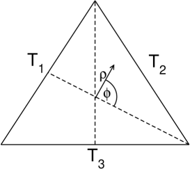
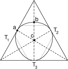
a)					b)

Figure F.1: The Dalitz-plot for $K_{L}\to 3\pi^{0}$ decay. In Fig. a), we display the polar coordinates, with $\rho\doteq Q\,r/3$. The physical region for the decay is bounded by the curve displayed in Eq. (F.2), shown in b) with a solid line. The three dotted lines denote the location of the cusps at $s_{i}=4M_{\pi}^{2}$. By a proper choice of the outgoing momenta of the pions, all events may be mapped into the region $abc$.

In Fig. F.2, we show the differential phase space in the standard case where the full phase space is used, and in the case where the events are mapped into the triangle $abc$. Although the integrated phase space is of course identical in the two cases, their shape is very different.

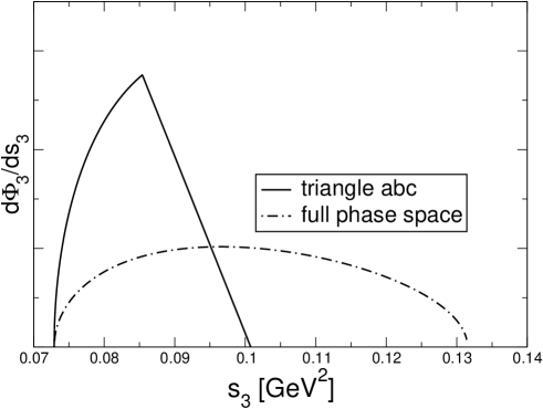
Figure F.2: The differential phase space $d\Phi_{3}/ds_{3}$. Its shape depends on the region chosen. The dash-dotted line is the standard full phase space region. The solid line corresponds to the case where all events are mapped into the triangle $abc$, see Fig. F.1b).

In the main text, we use the variables $s_{3}$, $\phi$ and restrict the phase space to the triangle $abc$. Note that by this procedure, the number of neutral pion pairs located in the vicinity of the cusp region is increased by a factor of 3.

References

- [1] E. P. Wigner, Phys. Rev. 73 (1948) 1002.
- [2] P. Budini and L. Fonda, Phys. Rev. Lett. 6 (1961) 419.
- [3] N. Cabibbo, Phys. Rev. Lett. 93 (2004) 121801 [arXiv:hep-ph/0405001].
- [4] N. Cabibbo and G. Isidori, JHEP 0503 (2005) 021 [arXiv:hep-ph/0502130].
- [5] E. Gámiz, J. Prades and I. Scimemi, Eur. Phys. J. C 50 (2007) 405 [arXiv:hep-ph/0602023].
- [6] G. Colangelo, J. Gasser, B. Kubis and A. Rusetsky, Phys. Lett. B 638 (2006) 187 [arXiv:hep-ph/0604084].
- [7] M. Bissegger, A. Fuhrer, J. Gasser, B. Kubis and A. Rusetsky, Phys. Lett. B 659 (2008) 576 [arXiv:0710.4456 [hep-ph]].
- [8] U.-G. Meißner, G. Müller and S. Steininger, Phys. Lett. B 406 (1997) 154 [Erratum-ibid. B 407 (1997) 454] [arXiv:hep-ph/9704377].
- [9] J. R. Batley et al. [NA48/2 Collaboration], Phys. Lett. B 633 (2006) 173 [arXiv:hep-ex/0511056].
- [10] L. Di Lella, Review of scattering measurements in decays, talk given at: Kaon’07, May 21–25, 2007, Frascati, Italy.
- [11] D. Madigozhin, Pion scattering lengths from the cusp effect analysis, talk given at: FlaviAnet Kaon Workshop, June 12–14, 2008, Anacapri, Italy.
-
[12]
For talks provided by members of the NA48/2 collaboration, see
http://na48.web.cern.ch/NA48/Welcome/images/talks.html. - [13] E. Abouzaida et al. [KTeV Collaboration], arXiv:0806.3535 [hep-ex].
- [14] L. Rosselet et al., Phys. Rev. D 15 (1977) 574.
- [15] S. Pislak et al., Phys. Rev. D 67 (2003) 072004 [arXiv:hep-ex/0301040].
- [16] J. R. Batley et al. [NA48/2 Collaboration], Eur. Phys. J. C 54 (2008) 411.
- [17] B. Bloch-Devaux, Results from NA48/2 in Ke4 decays: Form factors and scattering lengths, talk given at: FlaviAnet Kaon Workshop, June 12–14, 2008, Anacapri, Italy.
- [18] B. Adeva et al. [DIRAC Collaboration], J. Phys. G 30 (2004) 1929 [arXiv:hep-ex/0409053].
- [19] B. Adeva et al. [DIRAC Collaboration], Phys. Lett. B 619 (2005) 50 [arXiv:hep-ex/0504044].
- [20] G. Colangelo, J. Gasser and H. Leutwyler, Phys. Lett. B 488 (2000) 261 [arXiv:hep-ph/0007112].
- [21] G. Colangelo, J. Gasser and H. Leutwyler, Nucl. Phys. B 603 (2001) 125 [arXiv:hep-ph/0103088].
- [22] A. Nehme, Phys. Rev. D 70 (2004) 094025 [arXiv:hep-ph/0406209].
- [23] J. Bijnens and F. Borg, Eur. Phys. J. C 39 (2005) 347 [arXiv:hep-ph/0410333].
- [24] J. Bijnens and F. Borg, Eur. Phys. J. C 40 (2005) 383 [arXiv:hep-ph/0501163].
- [25] G. Isidori, Eur. Phys. J. C 53 (2008) 567 [arXiv:0709.2439 [hep-ph]].
- [26] S. R. Gevorkyan, A. V. Tarasov and O. O. Voskresenskaya, Phys. Lett. B 649 (2007) 159 [arXiv:hep-ph/0612129].
- [27] S. R. Gevorkyan, D. T. Madigozhin, A. V. Tarasov and O. O. Voskresenskaya, Phys. Part. Nucl. Lett. 5 (2008) 85 [arXiv:hep-ph/0702154].
- [28] M. Beneke and V. A. Smirnov, Nucl. Phys. B 522 (1998) 321 [arXiv:hep-ph/9711391].
- [29] J. Gasser, V. E. Lyubovitskij, A. Rusetsky and A. Gall, Phys. Rev. D 64 (2001) 016008 [arXiv:hep-ph/0103157].
- [30] J. Gasser, V. E. Lyubovitskij and A. Rusetsky, Phys. Rept. 456 (2008) 167 [arXiv:0711.3522 [hep-ph]].
- [31] J. Gasser, B. Kubis and A. Rusetsky, in preparation.
- [32] J. L. Goity, D. Lehmann, G. Prézeau and J. Saez, Phys. Lett. B 504 (2001) 21 [arXiv:hep-ph/0101011].
- [33] D. Lehmann and G. Prézeau, Phys. Rev. D 65 (2002) 016001 [arXiv:hep-ph/0102161].
- [34] M. Knecht and R. Urech, Nucl. Phys. B 519 (1998) 329 [arXiv:hep-ph/9709348].
- [35] V. Antonelli, A. Gall, J. Gasser and A. Rusetsky, Annals Phys. 286 (2001) 108 [arXiv:hep-ph/0003118].
- [36] B. Kubis, PhD thesis, Berichte des FZ Jülich, Jül-4007 (2002).
- [37] Z. K. Silagadze, JETP Lett. 60 (1994) 689 [arXiv:hep-ph/9411382].
- [38] J. Kulpa and S. Wycech, Acta Phys. Polon. B 38 (2007) 2973.
- [39] S. Wycech and A. M. Green, Nucl. Phys. A 562 (1993) 446 [arXiv:hep-ph/9302293].
- [40] A. Gall, J. Gasser, V. E. Lyubovitskij and A. Rusetsky, Phys. Lett. B 462 (1999) 335 [arXiv:hep-ph/9905309].
- [41] J. Gasser, V. E. Lyubovitskij and A. Rusetsky, Phys. Lett. B 471 (1999) 244 [arXiv:hep-ph/9910438].
- [42] J. Schweizer, Phys. Lett. B 587 (2004) 33 [arXiv:hep-ph/0401048].
- [43] J. Schweizer, Eur. Phys. J. C 36 (2004) 483 [arXiv:hep-ph/0405034].
- [44] J. Schwinger, J. Math. Phys. 5 (1964) 1606.
- [45] J. Gasser, B. Kubis and A. Rusetsky, private communication to the NA48 collaboration.
- [46] W. M. Yao et al. [Particle Data Group], J. Phys. G 33 (2006) 1, and 2007 partial update for the 2008 edition.
- [47] R. H. Dalitz, Phil. Mag. 44 (1953) 1068.
- [48] E. Fabri, Nuovo Cim. 11 (1954) 479.