A subtraction scheme for computing QCD jet cross sections at NNLO: integrating the subtraction terms I.

Abstract:

In previous articles we outlined a subtraction scheme for regularizing doubly-real emission and real-virtual emission in next-to-next-to-leading order (NNLO) calculations of jet cross sections in electron-positron annihilation. In order to find the NNLO correction these subtraction terms have to be integrated over the factorized unresolved phase space and combined with the two-loop corrections. In this paper we perform the integration of all one-parton unresolved subtraction terms.

1 Introduction

In recent years a lot of effort has been devoted to extending the subtraction method of computing QCD corrections at the next-to-leading order (NLO) accuracy to the computation of the radiative corrections at the next-to-next-to-leading order (NNLO) [1, 2, 3, 4, 5, 6, 7, 8, 9, 10, 11]. In particular, in Ref. [10], a subtraction scheme was defined for computing NNLO corrections to QCD jet cross sections to processes without coloured partons in the initial state and arbitrary number of massless particles (coloured or colourless) in the final state. That scheme can be summarized as follows.

The NNLO correction to any $m$-jet cross section of processes without coloured partons in the initial state is a sum of three contributions, the doubly-real, the one-loop singly-unresolved real-virtual and the two-loop doubly-virtual terms,

$$\sigma^{\mathrm{NNLO}}=\int_{m+2}\!{\mathrm{d}}\sigma^{{\rm RR}}_{m+2}J_{m+2}+\int_{m+1}\!{\mathrm{d}}\sigma^{{\rm RV}}_{m+1}J_{m+1}+\int_{m}\!{\mathrm{d}}\sigma^{{\rm VV}}_{m}J_{m}\>.$$ (1.1)

Here the notation for the integrals indicates that the doubly-real corrections involve the fully-differential cross section ${\mathrm{d}}\sigma^{{\rm RR}}_{m+2}$ of $m+2$ final-state partons, the real-virtual contribution involves the fully-differential cross section for the production of $m+1$ final-state partons at one-loop and the doubly-virtual term is an integral of the fully-differential cross section for the production of $m$ final-state partons at two-loops. The phase spaces are restricted by the corresponding jet functions $J_{n}$ that define the physical quantity.

In $d=4$ dimensions the three contributions in Eq. (1.1) are separately divergent, but their sum is finite for infrared-safe observables. (The requirement of infrared safety implies certain analytic properties of the jet functions $J_{n}$ that are spelled out in Ref. [8].) As explained in Ref. [10] we first continue analytically all integrals to $d=4-2\epsilon$ dimensions and then rewrite Eq. (1.1) as

$$\sigma^{\mathrm{NNLO}}=\int_{m+2}\!{\mathrm{d}}\sigma^{{\rm NNLO}}_{m+2}+\int_{m+1}\!{\mathrm{d}}\sigma^{{\rm NNLO}}_{m+1}+\int_{m}\!{\mathrm{d}}\sigma^{{\rm NNLO}}_{m}\,,$$ (1.2)

that is a sum of integrals,

$${\mathrm{d}}\sigma^{{\rm NNLO}}_{m+2} = \Big{\{}{\mathrm{d}}\sigma^{{\rm RR}}_{m+2}J_{m+2}-{\mathrm{d}}\sigma^{{\rm RR,A}_{\scriptscriptstyle 2}}_{m+2}J_{m}-\Big{[}{\mathrm{d}}\sigma^{{\rm RR,A}_{\scriptscriptstyle 1}}_{m+2}J_{m+1}-{\mathrm{d}}\sigma^{{\rm RR,A}_{\scriptscriptstyle 12}}_{m+2}J_{m}\Big{]}\Big{\}}_{\epsilon=0}\,,$$ (1.3)

$${\mathrm{d}}\sigma^{{\rm NNLO}}_{m+1} = \Big{\{}\Big{[}{\mathrm{d}}\sigma^{{\rm RV}}_{m+1}+\int_{1}{\mathrm{d}}\sigma^{{\rm RR,A}_{\scriptscriptstyle 1}}_{m+2}\Big{]}J_{m+1}-\Big{[}{\mathrm{d}}\sigma^{{\rm RV,A}_{\scriptscriptstyle 1}}_{m+1}+\Big{(}\int_{1}{\mathrm{d}}\sigma^{{\rm RR,A}_{\scriptscriptstyle 1}}_{m+2}\Big{)}^{{\rm A}_{\scriptscriptstyle 1}}\Big{]}J_{m}\Big{\}}_{\epsilon=0}\,,\;\;\;\;\;\;$$ (1.4)

and

$${\mathrm{d}}\sigma^{{\rm NNLO}}_{m}=\Big{\{}{\mathrm{d}}\sigma^{{\rm VV}}_{m}+\int_{2}\Big{[}{\mathrm{d}}\sigma^{{\rm RR,A}_{\scriptscriptstyle 2}}_{m+2}-{\mathrm{d}}\sigma^{{\rm RR,A}_{\scriptscriptstyle 12}}_{m+2}\Big{]}+\int_{1}\Big{[}{\mathrm{d}}\sigma^{{\rm RV,A}_{\scriptscriptstyle 1}}_{m+1}+\Big{(}\int_{1}{\mathrm{d}}\sigma^{{\rm RR,A}_{\scriptscriptstyle 1}}_{m+2}\Big{)}^{{\rm A}_{\scriptscriptstyle 1}}\Big{]}\Big{\}}_{\epsilon=0}J_{m}\,,$$ (1.5)

each integrable in four dimensions by construction. The forms of the subtraction terms in Eqs. (1.3) and (1.4) are symbolic in the sense that each approximate cross section is actually a sum of many terms. The jet function depends on different momenta in each of those terms; the exact set of momenta for each term can be found in Refs. [10, 12]. In Eq. (1.3) ${\mathrm{d}}\sigma^{{\rm RR,A}_{\scriptscriptstyle 1}}_{m+2}$ and ${\mathrm{d}}\sigma^{{\rm RR,A}_{\scriptscriptstyle 2}}_{m+2}$ are approximate cross sections that regularize the doubly-real emission cross section in the one- and two-parton infrared regions of the phase space, respectively. The double subtraction due to the overlap of these two terms is compensated by ${\mathrm{d}}\sigma^{{\rm RR,A}_{\scriptscriptstyle 12}}_{m+2}$. These terms are defined in Ref. [10] explicitly, where the finiteness of ${\mathrm{d}}\sigma^{{\rm NNLO}}_{m+2}$ is demonstrated also numerically for the case of $e^{+}e^{-}\to 3$ jets ($m=3$). In Ref. [13], we computed the integral $\int_{1}{\mathrm{d}}\sigma^{{\rm RR,A}_{\scriptscriptstyle 1}}_{m+2}$ and showed that the terms in the first bracket in Eq. (1.4) do not contain $\epsilon$ poles. Nevertheless, those terms still lead to divergent integrals due to kinematical singularities in the one-parton unresolved parts of the phase space. In Ref. [12] we defined explicitly ${\mathrm{d}}\sigma^{{\rm RV,A}_{\scriptscriptstyle 1}}_{m+1}$ and $\Big{(}\int_{1}{\mathrm{d}}\sigma^{{\rm RR,A}_{\scriptscriptstyle 1}}_{m+2}\Big{)}^{{\rm A}_{\scriptscriptstyle 1}}$, that regularize the singly-unresolved limits of the real-virtual cross section and $\int_{1}{\mathrm{d}}\sigma^{{\rm RR,A}_{\scriptscriptstyle 1}}_{m+2}$ in turn and demonstrated the finiteness of the regularized cross section ${\mathrm{d}}\sigma^{{\rm NNLO}}_{m+1}$ for the example of $e^{+}e^{-}\to 3$ jets. Thus all formulae relevant for constructing ${\mathrm{d}}\sigma^{{\rm NNLO}}_{m+2}$ and ${\mathrm{d}}\sigma^{{\rm NNLO}}_{m+1}$ explicitly are available.

In order to finish the definition of the subtraction scheme, one has to compute the integrals over the factorized one- and two-parton phase spaces, indicated in Eq. (1.5). Those integrals have to be computed in $d$ dimensions and the results have to be presented in the form of a Laurent expansion in $\epsilon$. According to the KLN theorem, the $\epsilon$ poles in the expansions have to cancel those in the two-loop contribution ${\mathrm{d}}\sigma^{{\rm VV}}_{m}$, leading to a finite cross section ${\mathrm{d}}\sigma^{{\rm NNLO}}_{m}$, that can be integrated in four dimensions. In this paper we compute the $\epsilon$-expansion of the one-particle integrals, denoted formally by $\int_{1}$, that appear in Eqs. (1.4) and (1.5). Once these are known, the only missing ingredient for a complete scheme for computing NNLO corrections is the $\epsilon$-expansion of the two-particle integrals, denoted formally by $\int_{2}$ in Eq. (1.5).

There are several ways to compute the one-particle integrals. If the singular integrals in the chosen integration variables are non-overlapping and occur in a single point in the integration region (which can always be mapped to the origin), then one can isolate the poles using standard residuum subtraction, leading to integrals of smooth functions that can easily be evaluated numerically. In most integrals we encounter, there are overlapping singularities in some variables and/or some variables lead to singular integrals in two points of the integration region. In the latter case, the integral can be written as a sum of two integrals with singularity in a single point, while the overlaps can be disentangled using sector decomposition [15], so that residuum subtraction can be applied. We have written a Mathematica program for the extraction of the poles employing these techniques. The program produces Fortran codes that can be immediately used in a Monte Carlo integration program such as those in the Cuba library [17]. We used the program SectorDecompisition of Ref. [16] to check our integrations. The integrated subtraction terms are smooth functions of a single kinematical variable (in one case three variables) and some parameters.

One can also extend the method of differential equations [18], developed for computing multi-loop Feynman integrals [19], to the relevant phase-space integrations. This leads to $\epsilon$-expansions with analytic, though rather cumbersome coefficients. We have used this method for computing some of the singly-unresolved integrals of the approximate real-virtual cross section and found numerical agreement with the results of residuum subtraction [20].

A third way to obtain the one-particle integrals is to use the Mellin-Barnes (MB) technique [21, 22, 23] to compute them, leading to $\epsilon$-expansions with analytic coefficients. The singly-unresolved integrals defined in this paper have also been computed via deriving MB representations and using the MB [24] Mathematica program for obtaining the analytic continuations and then the coefficients of $\epsilon$-expansions [25].

All integrals presented in this paper have been obtained by at least two independent computations.

In the next section we set some basic notation used in the rest of the paper. In general we adopt the colour- and spin-state notation of Ref. [14] and the notation for defining the various cross sections introduced in Refs. [8, 10, 12]. In Sect. 3 we compute the integral of the doubly-real singly-unresolved counterterms up to $\mathrm{O}(\epsilon^{2})$ accuracy. Sects. 4 and 5 repeat the same computations to $\mathrm{O}(\epsilon^{0})$ for the real-virtual counterterms and for the counterterms of the integrated approximate cross section, respectively. These integrations are very similar to that in Sect. 3, therefore, the structure of these sections is the same as that of Sect. 3, only the actual expressions differ. Sect. 6 contains our conclusions.

2 Notation

2.1 Matrix elements

We consider processes with coloured particles (partons) in the final states, while the initial-state particles are colourless (typically electron-positron annihilation into hadrons). Any number of additional non-coloured final-state particles is allowed, too, but they will be suppressed in the notation. Resolved partons in the final state are labeled by $i,k,l,\dots$, the unresolved one is denoted by $r$.

We adopt the colour- and spin-state notation of Ref. [14]. In this notation the amplitude for a scattering process involving the final-state momenta $\{p\}$, $|{\cal M}_{m}(\{p\})\rangle$, is an abstract vector in colour and spin space, and its normalization is fixed such that the squared amplitude summed over colours and spins is

$$|{\cal M}_{m}|^{2}=\langle{\cal M}_{m}||{\cal M}_{m}\rangle\>.$$ (2.1)

This matrix element has the following formal loop expansion:

$$|{\cal M}\rangle=|{\cal M}^{(0)}\rangle+|{\cal M}^{(1)}\rangle+\dots\,,$$ (2.2)

where $|{\cal M}^{(0)}\rangle$ denotes the tree-level contribution, $|{\cal M}^{(1)}\rangle$ is the one-loop contribution and the dots stand for higher-loop contributions, which are not used in this paper.

Colour interactions at QCD vertices are represented by associating colour charges ${\mbox{\boldmath$T$}}_{i}$ with the emission of a gluon from each parton $i$. In the colour-state notation, each vector $|{\cal M}\rangle$ is a colour-singlet state, so colour conservation is simply

$$\biggl{(}\sum_{j}{\mbox{\boldmath$T$}}_{j}\biggr{)}\,|{\cal M}\rangle=0\,,$$ (2.3)

where the sum over $j$ extends over all the external partons of the state vector $|{\cal M}\rangle$, and the equation is valid order by order in the loop expansion of Eq. (2.2).

Using the colour-state notation, we define the two-parton colour-correlated squared tree amplitudes as

$$|{\cal M}^{(0)}_{(i,k)}(\{p\})|^{2}\equiv\langle{\cal M}^{(0)}(\{p\})|\,{\mbox{\boldmath$T$}}_{i}\!\cdot\!{\mbox{\boldmath$T$}}_{k}\,|{\cal M}^{(0)}(\{p\})\rangle$$ (2.4)

and similarly the three-parton colour-correlated squared tree amplitudes, $|{\cal M}^{(0)}_{(i,k,l)}|^{2}$ for $i$, $k$ and $l$ being different,

$$|{\cal M}^{(0)}_{(i,k,l)}|^{2}\equiv\sum_{a,b,c}f_{abc}\langle{\cal M}^{(0)}|T^{a}_{i}T^{b}_{k}T^{c}_{l}|{\cal M}^{(0)}\rangle\,.$$ (2.5)

The colour-charge algebra for the product $({\mbox{\boldmath$T$}}_{i})^{n}({\mbox{\boldmath$T$}}_{k})^{n}\equiv{\mbox{\boldmath$T$}}_{i}\!\cdot\!{\mbox{\boldmath$T$}}_{k}$ is:

$${\mbox{\boldmath$T$}}_{i}\!\cdot\!{\mbox{\boldmath$T$}}_{k}={\mbox{\boldmath$T$}}_{k}\!\cdot\!{\mbox{\boldmath$T$}}_{i}\quad{\rm if}\quad i\neq k;\qquad{\mbox{\boldmath$T$}}_{i}^{2}=C_{i}\>.$$ (2.6)

Here $C_{i}$ is the quadratic Casimir operator in the representation of particle $i$ and we have $C_{\mathrm{F}}=T_{\mathrm{R}}(N_{\mathrm{c}}^{2}-1)/N_{\mathrm{c}}=(N_{\mathrm{c}}^{2}-1)/(2N_{\mathrm{c}})$ in the fundamental and $C_{\mathrm{A}}=2\,T_{\mathrm{R}}N_{\mathrm{c}}=N_{\mathrm{c}}$ in the adjoint representation, i.e. we are using the customary normalization $T_{\mathrm{R}}=1/2$.

2.2 Cross sections

In writing the final results in our notation we shall use the following cross sections:

• the Born cross section of producing $m$ final-state partons,

  $${\mathrm{d}}\sigma^{{\rm B}}_{m}={\cal N}\;\sum_{\{m\}}{\mathrm{d}}\phi_{m}{(\{p\})}\frac{1}{S_{\{m\}}}|{\cal M}_{m}^{(0)}{(\{p\})}|^{2}\,,$$ (2.7)

• the Born cross section of producing $m+1$ final-state partons, called real correction,

  $${\mathrm{d}}\sigma^{{\rm R}}_{m+1}={\cal N}\sum_{\{m+1\}}{\mathrm{d}}\phi_{m+1}{(\{p\})}\frac{1}{S_{\{m+1\}}}|{\cal M}_{m+1}^{(0)}{(\{p\})}|^{2}\,,$$ (2.8)

• and the one-loop correction ${\mathrm{d}}\sigma^{{\rm V}}_{m}$ to the $m$-parton Born cross section, called virtual correction,

  $${\mathrm{d}}\sigma^{{\rm V}}_{m}={\cal N}\;\sum_{\{m\}}{\mathrm{d}}\phi_{m}{(\{p\})}\frac{1}{S_{\{m\}}}\>2\mathop{\mathrm{Re}}\nolimits\langle{\cal M}_{m}^{(0)}(\{p\})|{\cal M}_{m}^{(1)}(\{p\})\rangle\,,$$ (2.9)

where ${\cal N}$ includes all QCD-independent factors and ${\mathrm{d}}\phi_{n}{(\{p\})}$ is the $d$-dimensional phase space for $n$ outgoing particles with momenta $\{p\}\equiv\{p_{1},\dots,p_{n}\}$ and total momentum $Q$,

$${\mathrm{d}}\phi_{n}(p_{1},\ldots,p_{n};Q)=\prod_{i=1}^{n}\frac{{\mathrm{d}}^{d}p_{i}}{(2\pi)^{d-1}}\,\delta_{+}(p_{i}^{2})\,(2\pi)^{d}\delta^{(d)}\left(Q-\sum_{i=1}^{n}p_{i}\right)\,.$$ (2.10)

The symbol $\sum_{\{n\}}$ denotes summation over the different subprocesses and $S_{\{n\}}$ is the Bose symmetry factor for identical particles in the final state.

3 Integrals of the doubly-real singly-unresolved counterterms

The doubly-real singly-unresolved approximate cross section times the jet function reads

$${\mathrm{d}}\sigma^{{\rm RR,A}_{\scriptscriptstyle 1}}_{m+2}J_{m+1}={\cal N}\sum_{\{m+2\}}{\mathrm{d}}\phi_{m+2}(\{p\})\frac{1}{S_{\{m+2\}}}$$

$$\qquad\times\sum_{r}\Bigg{[}\sum_{i\neq r}\frac{1}{2}{\cal C}_{ir}^{(0,0)}(\{p\})J_{m+1}(\{\tilde{p}\}^{(ir)})$$

$$\qquad\qquad\qquad+\left({\cal S}_{r}^{(0,0)}(\{p\})-\sum_{i\neq r}{\cal C}_{ir}^{~{}}{\cal S}_{r}^{(0,0)}(\{p\})\right)J_{m+1}(\{\tilde{p}\}^{(r)})\Bigg{]}\,.$$ (3.1)

The precise meaning of the counterterms ${\cal C}_{ir}^{(0,0)}$, ${\cal S}_{r}^{(0,0)}$ and ${\cal C}_{ir}^{~{}}{\cal S}_{r}^{(0,0)}$ and the definition of the tilded sets of momenta $\{\tilde{p}\}^{(ir)}$ and $\{\tilde{p}\}^{(r)}$ (arguments of the jet functions) were spelled out explicitly in Ref. [10]. The integral of this approximate cross section over the one-particle factorized phase space was presented in Ref. [13]. Nevertheless, we recompute it here for two reasons. On the one hand, we use slightly generalized subtraction terms, while on the other hand in a NNLO computation we need the expansion of the integrals up to $\mathrm{O}(\epsilon^{2})$ accuracy. In the following, we recall the definitions of the subtraction terms only to the extent needed to compute their integrals over the factorized phase spaces.

3.1 Integral of the collinear counterterm

The collinear counterterm reads

$$\begin{split}{\cal C}_{ir}^{(0,0)}(\{p\})&=8\pi\alpha_{\mathrm{s}}\mu^{2\epsilon}\frac{1}{s_{ir}}\langle{\cal M}_{m+1}^{(0)}(\{\tilde{p}\}^{(ir)})|\hat{P}_{f_{i}f_{r}}^{(0)}(z_{i,r},z_{r,i},k_{\perp,i,r};\epsilon)|{\cal M}_{m+1}^{(0)}(\{\tilde{p}\}^{(ir)})\rangle\\ &\times(1-\alpha_{ir})^{2d_{0}-2m(1-\epsilon)}\Theta(\alpha_{0}-\alpha_{ir})\,,\end{split}$$ (3.2)

where $s_{ir}=2p_{i}\!\cdot\!p_{r}$, $\hat{P}_{f_{i}f_{r}}^{(0)}$ is the Altarelli–Parisi splitting kernel in $d=4-2\epsilon$ dimensions for the splitting process $f\rightarrow f_{i}+f_{r}$ and $\alpha_{0}\in(0,1]$. The momentum fractions are defined as

$$z_{i,r}=\frac{y_{iQ}}{y_{(ir)Q}}\qquad\mbox{and}\qquad z_{r,i}=\frac{y_{rQ}}{y_{(ir)Q}}\,,$$ (3.3)

where $y_{jQ}=s_{jQ}/Q^{2}=2p_{j}\!\cdot\!Q/Q^{2}$, ($j=i,\,r$ etc.) and $y_{(ir)Q}=y_{iQ}+y_{rQ}$. With this definition, we clearly have $z_{i,r}+z_{r,i}=1$. In order to render the integrated counterterm $m$-independent (see Eq. (3.6) below) and to reduce the CPU time necessary for the numerical integration, we have included two harmless factors in the second line of Eq. (3.2) as compared to the original definitions in Ref. [10]. We give a detailed discussion of these modifications in Appendix A.

The matrix elements on the right hand side of Eq. (3.2) are evaluated with the $m+1$ momenta $\{\tilde{p}\}^{(ir)}=\{\tilde{p}_{1},\ldots,\tilde{p}_{ir},\ldots,\tilde{p}_{m+2}\}$, that are defined by a specific mapping,

$$\{p\}\stackrel{{\scriptstyle{\mathsf{C}}_{ir}}}{{\longrightarrow}}\{\tilde{p}\}^{(ir)}\,,$$ (3.4)

of the original $m+2$ momenta $\{p\}$. This mapping leads to an exact factorization of the $(m+2)$-particle phase space such that we have

$${\mathrm{d}}\phi_{m+2}(\{p\};Q)={\mathrm{d}}\phi_{m+1}(\{\tilde{p}\}^{(ir)};Q)\>[{\mathrm{d}}p_{1;m+1}^{(ir)}(p_{r},\tilde{p}_{ir};Q)]\,.$$ (3.5)

We write the result of integrating the collinear subtraction term as given in Eq. (3.2) over the factorized phase space $[{\mathrm{d}}p_{1;m+1}^{(ir)}]$ in the following form:

$$\int_{1}{\cal C}_{ir}^{(0,0)}(\{p\})=\frac{\alpha_{\mathrm{s}}}{2\pi}\,S_{\epsilon}\left(\frac{\mu^{2}}{Q^{2}}\right)^{\epsilon}{\mathrm{C}}_{ir}^{(0)}(y_{\widetilde{\,ir\,}Q};\epsilon)\,{\mbox{\boldmath$T$}}_{ir}^{2}\,|{\cal M}_{m+1}^{(0)}{(\{\tilde{p}\}^{(ir)})}|^{2}\,,$$ (3.6)

where

$$S_{\epsilon}=\int\!\frac{{\mathrm{d}}^{(d-3)}\Omega}{(2\pi)^{d-3}}=\frac{(4\pi)^{\epsilon}}{\Gamma(1-\epsilon)}\,,$$ (3.7)

$y_{\widetilde{\,ir\,}Q}\equiv s_{\widetilde{\,ir\,}Q}/Q^{2}=2\tilde{p}_{ir}\!\cdot\!Q/Q^{2}$ and the arguments of the function ${\mathrm{C}}_{ir}^{(0)}(y_{\widetilde{\,ir\,}Q};\epsilon)$ indicate that this function is independent of $m$. In order to lighten the notation throughout the paper we do not show the explicit dependence of ${\mathrm{C}}_{ir}^{(0)}$ on $\alpha_{0}$ and $d_{0}$.

The factorized phase space measure in Eq. (3.5) may be written in several equivalent ways. In this paper choose the form of a convolution:

$$[{\mathrm{d}}p_{1;m+1}^{(ir)}(p_{r},\tilde{p}_{ir};Q)]=\int_{0}^{1}\!{\mathrm{d}}\alpha_{ir}\,(1-\alpha_{ir})^{2m(1-\epsilon)-1}\,\frac{s_{\widetilde{\,ir\,}Q}}{2\pi}\,{\mathrm{d}}\phi_{2}(p_{i},p_{r};p_{(ir)})\,,$$ (3.8)

where $p_{(ir)}^{\mu}=(1-\alpha_{ir})\tilde{p}_{ir}^{\mu}+\alpha_{ir}Q^{\mu}$. The collinear momentum mapping and the implied factorization of the phase space measure are represented graphically in Fig. 1.

Figure 1: Graphical representation of the collinear momentum mapping and the implied phase space factorization.

The picture on the left shows the $(m+2)$-particle phase space ${\mathrm{d}}\phi_{m+2}(\{p\};Q)$, where in the circle we have indicated the number of momenta. The picture on the right corresponds to Eqs. (3.5) and (3.8): the two circles represent the $(m+1)$-particle phase space ${\mathrm{d}}\phi_{m+1}(\{\tilde{p}\}^{(ir)};Q)$ and the two-particle phase space ${\mathrm{d}}\phi_{2}(p_{i},p_{r};p_{(ir)})$ respectively, while the symbol $\otimes$ stands for the convolution over $\alpha_{ir}$, as precisely defined in Eq. (3.8).

With the chosen form of the factorized phase-space measure in Eq. (3.8), we can express the functions ${\mathrm{C}}_{ir}^{(0)}$ as

$$\begin{split}&{\mathrm{C}}_{ir}^{(0)}(y_{\widetilde{\,ir\,}Q};\epsilon)=\frac{(4\pi)^{2}}{S_{\epsilon}}(Q^{2})^{\epsilon}\\ &\qquad\times\int_{0}^{\alpha_{0}}\!{\mathrm{d}}\alpha\,(1-\alpha)^{2d_{0}-1}\frac{s_{\widetilde{\,ir\,}Q}}{2\pi}{\mathrm{d}}\phi_{2}(p_{i},p_{r};p_{(ir)})\frac{1}{s_{ir}}P_{f_{i}f_{r}}^{(0)}(z_{i,r},z_{r,i};\epsilon)\frac{1}{{\mbox{\boldmath$T$}}_{ir}^{2}}\,.\end{split}$$ (3.9)

In writing the right hand side of Eq. (3.9) we have used that because $k_{\perp,i,r}$ as defined in Ref. [12] is orthogonal to $\tilde{p}_{ir}$, the spin correlations generally present in Eq. (3.2) vanish after azimuthal integration. Therefore, we may replace the splitting kernels $\hat{P}_{f_{i}f_{r}}^{(0)}$ by their azimuthally averaged counterparts $P_{f_{i}f_{r}}^{(0)}$ when integrating the subtraction term over the factorized phase space. These spin-averaged splitting kernels depend, in general, on $z_{i,r}$ and $z_{r,i}$, with the constraint

$$z_{i,r}+z_{r,i}=1\,,$$ (3.10)

and are listed in Appendix B. The phase-space measure is symmetric under the $i\leftrightarrow r$ interchange, thus integrals containing integrands that are linear combinations of ratios of the momentum fractions, as in Eq. (3.9), can be expressed as linear combinations of integrals with integrands depending only on $z_{r,i}^{k}$. Therefore, we need to evaluate the following integrals:

$$\,\frac{(4\pi)^{2}}{S_{\epsilon}}(Q^{2})^{\epsilon}\,\int_{0}^{\alpha_{0}}\!{\mathrm{d}}\alpha_{ir}\,(1-\alpha_{ir})^{2d_{0}-1}\,\frac{s_{\widetilde{\,ir\,}Q}}{2\pi}\int\!{\mathrm{d}}\phi_{2}(p_{i},p_{r};p_{(ir)})\,\frac{z_{r,i}^{k}}{s_{ir}}\,,$$ (3.11)

for the values $k=-1,0,1,2$. As explained in the introduction, in this paper we use sector decomposition and residuum subtraction to compute the $\varepsilon$-expansion of Eq. (3.11). It is also possible to evaluate these integrals analytically. The details are given in Ref. [20].

3.2 Integrals of the soft-type counterterms

We refer to the soft and soft-collinear counterterms together as soft-type because they both use the momentum mapping appropriate to the soft subtraction term. We define these counterterms as follows (note again the harmless factors as compared to the definitions in Ref. [10])

$${\cal S}_{r}^{(0,0)}(\{p\}) =-8\pi\alpha_{\mathrm{s}}\mu^{2\epsilon}\sum_{i}\sum_{k\neq i}\frac{1}{2}{\cal S}_{ik}(r)|{\cal M}_{m+1;(i,k)}^{(0)}{(\{\tilde{p}\}^{(r)})}|^{2}$$

$$\times(1-y_{rQ})^{d^{\prime}_{0}-m(1-\epsilon)}\Theta(y_{0}-y_{rQ})\,,$$ (3.12)

$${\cal C}_{ir}^{~{}}{\cal S}_{r}^{(0,0)}(\{p\}) =8\pi\alpha_{\mathrm{s}}\mu^{2\epsilon}\frac{1}{s_{ir}}\frac{2z_{i,r}}{z_{r,i}}\,{\mbox{\boldmath$T$}}_{i}^{2}\,|{\cal M}_{m+1}^{(0)}{(\{\tilde{p}\}^{(r)})}|^{2}$$

$$\times(1-y_{rQ})^{d^{\prime}_{0}-m(1-\epsilon)}\Theta(y_{0}-y_{rQ})\,,$$ (3.13)

where

$${\cal S}_{ik}(r)=\frac{2s_{ik}}{s_{ir}s_{kr}}\,,$$ (3.14)

and $y_{0}\in(0,1]$. The two-parton colour-correlated squared matrix element $|{\cal{M}}_{m+1;(i,k)}^{(0)}|^{2}$ in Eq. (3.12) is defined in Eq. (2.4). The momentum fractions $z_{i,r}$ and $z_{r,i}$ were defined in Eq. (3.3). The matrix elements on the right hand sides of Eqs. (3.12) and (3.13) are evaluated with the $m+1$ momenta $\{\tilde{p}\}^{(r)}=\{\tilde{p}_{1},\ldots,\tilde{p}_{m+2}\}$ ($p_{r}$ is missing from the set), obtained from the original $m+2$ momenta, $\{p\}$, by a mapping,

$$\{p\}\stackrel{{\scriptstyle{\mathsf{S}}_{r}}}{{\longrightarrow}}\{\tilde{p}\}^{(r)}\,.$$ (3.15)

This mapping leads to an exact factorization of the $(m+2)$-particle phase space,

$${\mathrm{d}}\phi_{m+2}(\{p\};Q)={\mathrm{d}}\phi_{m+1}(\{\tilde{p}\}^{(r)};Q)\>[{\mathrm{d}}p_{1;m+1}^{(r)}(p_{r};Q)]\,.$$ (3.16)

We write the result of integrating the soft-type subtraction terms over the factorized phase space $[{\mathrm{d}}p_{1;m+1}^{(r)}]$ as follows:

$$\int_{1}{\cal S}_{r}^{(0,0)}(\{p\}) =\frac{\alpha_{\mathrm{s}}}{2\pi}\,S_{\epsilon}\left(\frac{\mu^{2}}{Q^{2}}\right)^{\epsilon}\sum_{i}\sum_{k\neq i}{\mathrm{S}}_{ik}^{(0)}(Y_{\tilde{i}\tilde{k},Q};\epsilon)|{\cal M}_{m+1;(i,k)}^{(0)}{(\{\tilde{p}\}^{(r)})}|^{2}\,,$$ (3.17)

$$\int_{1}{\cal C}_{ir}{\cal S}_{r}^{(0,0)}(\{p\}) =\frac{\alpha_{\mathrm{s}}}{2\pi}\,S_{\epsilon}\left(\frac{\mu^{2}}{Q^{2}}\right)^{\epsilon}\mathrm{CS}^{(0)}(\epsilon)\,{\mbox{\boldmath$T$}}_{i}^{2}\,|{\cal M}_{m+1}^{(0)}{(\{\tilde{p}\}^{(r)})}|^{2}\,.$$ (3.18)

The functions ${\mathrm{S}}_{ik}^{(0)}(Y_{\tilde{i}\tilde{k},Q};\epsilon)$ and $\mathrm{CS}^{(0)}(\epsilon)$ are again independent of $m$ as the arguments indicate and as before, we lighten the notation throughout by not showing the explicit dependence of the integrated subtraction terms on $y_{0}$ and $d^{\prime}_{0}$. Also, ${\mathrm{S}}_{ik}^{(0)}(Y_{\tilde{i}\tilde{k},Q};\epsilon)$ only depends on the combination of variables

$$Y_{\tilde{i}\tilde{k},Q}=\frac{y_{\tilde{i}\tilde{k}}}{y_{\tilde{i}Q}y_{\tilde{k}Q}}\,.$$ (3.19)

As in the collinear case, the one-particle factorized phase space may also be written in the form of a convolution

$$[{\mathrm{d}}p_{1;m+1}^{(r)}(p_{r};Q)]=\int_{0}^{1}{\mathrm{d}}y_{rQ}(1-y_{rQ})^{m(1-\epsilon)-1}\frac{Q^{2}}{2\pi}{\mathrm{d}}\phi_{2}(p_{r},K;Q)$$ (3.20)

where the timelike momentum $K$ is massive with $K^{2}=(1-y_{rQ})Q^{2}$. We show the soft momentum mapping and the implied phase space factorization in Fig. 2.

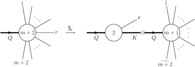
Figure 2: Graphical representation of the soft momentum mapping and the implied phase space factorization.

The picture on the left shows again the $(m+2)$-particle phase space ${\mathrm{d}}\phi_{m+2}(\{p\};Q)$, while the picture on the right corresponds to Eqs. (3.16) and (3.20): the two circles represent the two-particle phase space ${\mathrm{d}}\phi_{2}(p_{r},K;Q)$ and the $(m+1)$-particle phase space ${\mathrm{d}}\phi_{m+1}(\{\tilde{p}\}^{(r)};Q)$ respectively. The symbol $\otimes$ stands for the convolution over $y_{rQ}$ as defined in Eq. (3.20).

Using the definition of the subtraction terms in Eqs. (3.12) and (3.13) and the chosen form of the factorized phase space, we find that the functions ${\mathrm{S}}_{ik}^{(0)}(Y_{\tilde{i}\tilde{k},Q};\epsilon)$ and $\mathrm{CS}^{(0)}(\epsilon)$ can be written as

$${\mathrm{S}}_{ik}^{(0)}(Y_{\tilde{i}\tilde{k},Q};\epsilon) =-\frac{(4\pi)^{2}}{S_{\epsilon}}(Q^{2})^{\epsilon}\int_{0}^{y_{0}}\!{\mathrm{d}}y\,(1-y)^{d^{\prime}_{0}-1}\frac{Q^{2}}{2\pi}{\mathrm{d}}\phi_{2}(p_{r},K;Q)\frac{1}{2}{\cal S}_{ik}(r)$$ (3.21)

$$\mathrm{CS}^{(0)}(\epsilon) =\frac{(4\pi)^{2}}{S_{\epsilon}}(Q^{2})^{\epsilon}\int_{0}^{y_{0}}\!{\mathrm{d}}y\,(1-y)^{d^{\prime}_{0}-1}\frac{Q^{2}}{2\pi}{\mathrm{d}}\phi_{2}(p_{r},K;Q)\frac{1}{s_{ir}}\frac{2z_{i,r}}{z_{r,i}}\,.$$ (3.22)

The computation of these integrals is fairly straightforward using energy and angle variables. The details can be found in Ref. [20].

3.3 The integrated approximate cross section

We are now in a position to compute the integral of ${\mathrm{d}}\sigma^{{\rm RR,A}_{\scriptscriptstyle 1}}_{m+2}$ as given in Eq. (3.1) over the one-particle factorized phase space. In order to evaluate $\int_{1}{\mathrm{d}}\sigma^{{\rm RR,A}_{\scriptscriptstyle 1}}_{m+2}$ we first use the phase-space factorization properties of Eqs. (3.5) and (3.16), then perform the integration to obtain

$$\int_{1}{\mathrm{d}}\sigma^{{\rm RR,A}_{\scriptscriptstyle 1}}_{m+2}J_{m+1}={\cal N}\sum_{\{m+2\}}{\mathrm{d}}\phi_{m+1}(\{\tilde{p}\})\frac{1}{S_{\{m+2\}}}\frac{\alpha_{\mathrm{s}}}{2\pi}S_{\varepsilon}\left(\frac{\mu^{2}}{Q^{2}}\right)^{\varepsilon}$$

$$\qquad\times\sum_{r}\sum_{i\neq r}\Bigg{[}\frac{1}{2}{\mathrm{C}}_{ir}^{(0)}(y_{\widetilde{\,i\,}Q};\epsilon){\mbox{\boldmath$T$}}_{ir}^{2}|{\cal M}_{m+1}^{(0)}{(\{\tilde{p}\})}|^{2}J_{m+1}(\{\tilde{p}\})$$

$$\qquad\qquad\qquad\quad+\,\sum_{k\neq i,r}{\mathrm{S}}_{r}^{(0)}(Y_{\tilde{i}\tilde{k},Q};\epsilon)|{\cal M}_{m+1;(i,k)}^{(0)}{(\{\tilde{p}\})}|^{2}J_{m+1}(\{\tilde{p}\})$$

$$\qquad\qquad\qquad\quad\,-\mathrm{CS}^{(0)}(\epsilon){\mbox{\boldmath$T$}}_{i}^{2}|{\cal M}_{m+1}^{(0)}{(\{\tilde{p}\})}|^{2}J_{m+1}(\{\tilde{p}\})\Bigg{]}\,.$$ (3.23)

This result is not in the form of an $(m+1)$-parton configuration times a factor. In order to rewrite Eq. (3.23) in such a form, we need to perform the counting of symmetry factors for going from $m+1$ to $m+2$ partons. This was done in Appendix B of Ref. [13] for going from $m$ to $m+1$ partons and the results can readily be taken over by setting $m\to m+1$.

The final result for the integral of the doubly-real singly-unresolved approximate cross section can be written as [13]

$$\int_{1}{\mathrm{d}}\sigma^{{\rm RR,A}_{\scriptscriptstyle 1}}_{m+2}={\mathrm{d}}\sigma^{{\rm R}}_{m+1}\otimes{\mbox{\boldmath$I$}}^{(0)}(\{p\}_{m+1};\epsilon)\,,$$ (3.24)

where the insertion operator reads

$${\mbox{\boldmath$I$}}^{(0)}(\{p\}_{m+1};\epsilon)=\frac{\alpha_{\mathrm{s}}}{2\pi}\,S_{\epsilon}\left(\frac{\mu^{2}}{Q^{2}}\right)^{\epsilon}\\ \sum_{i}\bigg{[}{\mathrm{C}}_{i}^{(0)}(y_{iQ};\epsilon)\,{\mbox{\boldmath$T$}}_{i}^{2}+\sum_{k\neq i}\widetilde{{\mathrm{S}}}_{ik}^{(0)}(Y_{ik,Q};\epsilon)\,{\mbox{\boldmath$T$}}_{i}\!\cdot\!{\mbox{\boldmath$T$}}_{k}\bigg{]}\,.$$ (3.25)

In Eq. (3.25) we introduced the functions

$${\mathrm{C}}_{q}^{(0)}={\mathrm{C}}_{qg}^{(0)}\,,\qquad{\mathrm{C}}_{g}^{(0)}=\frac{1}{2}{\mathrm{C}}_{gg}^{(0)}+n_{\mathrm{f}}{\mathrm{C}}_{q{\bar{q}}}^{(0)}\,,\qquad\widetilde{{\mathrm{S}}}_{ik}^{(0)}={\mathrm{S}}_{ik}^{(0)}+\mathrm{CS}^{(0)}\,,$$ (3.26)

with ${\mathrm{C}}_{ir}^{(0)}$, ${\mathrm{S}}_{ik}^{(0)}$ and $\mathrm{CS}^{(0)}$ defined in Eqns. (3.9), (3.21) and (3.22), respectively. In this paper $n_{\mathrm{f}}$ denotes the number of light flavours, which we set to $n_{\mathrm{f}}=5$ in all numerical results. Upon expanding these functions in $\epsilon$ we find that the coefficients of the poles in the expansions are independent of the cut parameters $\alpha_{0}$ and $y_{0}$ as well as the exponents $d_{0}$ and $d^{\prime}_{0}$ and they read

$${\mathrm{C}}_{q}^{(0)}(x;\epsilon)=\frac{1}{\epsilon^{2}}+\frac{1}{\epsilon}\left(\frac{3}{2}-2\ln x\right)+\mathrm{O}(\epsilon^{0})\,,$$ (3.27)

$${\mathrm{C}}_{g}^{(0)}(x;\epsilon)=\frac{1}{\epsilon^{2}}+\frac{1}{\epsilon}\left(\frac{11}{6}-\frac{2}{3}n_{\mathrm{f}}\frac{T_{\mathrm{R}}}{C_{\mathrm{A}}}-2\ln x\right)+\mathrm{O}(\epsilon^{0})\,,$$ (3.28)

$$\widetilde{{\mathrm{S}}}_{ik}^{(0)}(Y;\epsilon)=\frac{1}{\epsilon}\ln Y+\mathrm{O}(\epsilon^{0})\,.$$ (3.29)

For the coefficients with non-negative powers of $\epsilon$ we obtain integral representations that can be evaluated numerically. The results for four values of $\alpha_{0}$ or $y_{0}=1$, $0.3$, $0.1$ and $0.03$ with fixed values of $d_{0}=d^{\prime}_{0}=3-3\varepsilon$ are presented in Figs. 3 and 4. The dependence on $\alpha_{0}$ in the collinear functions is hardly visible. Note also that the small-$x$ behaviour of the collinear functions is dominated by the logarithmic terms that are the same in the quark and gluon functions, therefore, the expansion coefficients of ${\mathrm{C}}_{q}^{(0)}(x;\varepsilon)$ and ${\mathrm{C}}_{g}^{(0)}(x;\varepsilon)$ are very similar.

Using colour-conservation (Eq. (2.3)), the definition of $Y_{\tilde{i}\tilde{k},Q}$ (3.19) and Eqs. (3.27)–(3.29) above, it is straightforward to verify that our insertion operator differs from that defined in Eq. (7.26) of Ref. [14] only in finite terms, i.e.

$${\mbox{\boldmath$I$}}^{(0)}(\{p\}_{n};\varepsilon)=\frac{\alpha_{\mathrm{s}}}{2\pi}S_{\varepsilon}\left(\frac{\mu^{2}}{Q^{2}}\right)^{\varepsilon}\sum_{i}\left({\mbox{\boldmath$T$}}_{i}^{2}\frac{1}{\varepsilon^{2}}+\gamma_{i}\frac{1}{\varepsilon}+\sum_{k\neq i}{\mbox{\boldmath$T$}}_{i}{\mbox{\boldmath$T$}}_{k}\frac{1}{\varepsilon}\ln y_{ik}\right)+\mathrm{O}(\epsilon^{0})\,,$$ (3.30)

with the usual flavour constants

$$\gamma_{q}=\frac{3}{2}C_{\mathrm{F}}\,\qquad\mbox{and}\qquad\gamma_{g}=\frac{\beta_{0}}{2}\,.$$ (3.31)

It follows that $\int_{1}{\mathrm{d}}\sigma^{{\rm RR,A}_{\scriptscriptstyle 1}}_{m+2}$ correctly cancels all $\varepsilon$-poles of the real-virtual cross section ${\mathrm{d}}\sigma^{{\rm RV}}_{m+1}$.

\psfrag{X}[ct]{$\log_{10}x$}\psfrag{Y}[cb]{\raisebox{5.0pt}{${\mathrm{C}}_{q}^{(0)}(x;\varepsilon)$}}\psfrag{T}[b]{\raisebox{5.0pt}{Order: $\varepsilon^{0}$}}\includegraphics[scale={0.42}]{figs/C0q_COL1_ep0.eps} \psfrag{X}[ct]{$\log_{10}x$}\psfrag{Y}{}\psfrag{T}[b]{\raisebox{5.0pt}{Order: $\varepsilon^{1}$}}\includegraphics[scale={0.42}]{figs/C0q_COL1_ep1.eps} \psfrag{X}[ct]{$\log_{10}x$}\psfrag{Y}{}\psfrag{T}[b]{\raisebox{5.0pt}{Order: $\varepsilon^{2}$}}\includegraphics[scale={0.42}]{figs/C0q_COL1_ep2.eps} \psfrag{X}[ct]{$\log_{10}x$}\psfrag{T}{}\psfrag{Y}[cb]{\raisebox{5.0pt}{${\mathrm{C}}_{g}^{(0)}(x;\varepsilon)$}}\includegraphics[scale={0.42}]{figs/C0g_COLsum_ep0.eps} \psfrag{X}[ct]{$\log_{10}x$}\psfrag{T}{}\psfrag{Y}{}\includegraphics[scale={0.42}]{figs/C0g_COLsum_ep1.eps} \psfrag{X}[ct]{$\log_{10}x$}\psfrag{T}{}\psfrag{Y}{}\includegraphics[scale={0.42}]{figs/C0g_COLsum_ep2.eps}

Figure 3: Expansion coeffiecients of the functions ${\mathrm{C}}_{i}^{(0)}(x;\varepsilon)$ with $d_{0}=3-3\varepsilon$ and $n_{\mathrm{f}}=5$. Upper row: $i=q$, lower row: $i=g$.

\psfrag{X}[ct]{$\log_{10}Y$}\psfrag{Y}[cb]{\raisebox{5.0pt}{$\widetilde{{\mathrm{S}}}_{ik}^{(0)}(Y;\varepsilon)$}}\psfrag{T}[b]{\raisebox{5.0pt}{Order: $\varepsilon^{0}$}}\includegraphics[scale={0.42}]{figs/Stilde0ik_COL1_ep0.eps} \psfrag{X}[ct]{$\log_{10}Y$}\psfrag{Y}{}\psfrag{T}[b]{\raisebox{5.0pt}{Order: $\varepsilon^{1}$}}\includegraphics[scale={0.42}]{figs/Stilde0ik_COL1_ep1.eps} \psfrag{X}[ct]{$\log_{10}Y$}\psfrag{Y}{}\psfrag{T}[b]{\raisebox{5.0pt}{Order: $\varepsilon^{2}$}}\includegraphics[scale={0.42}]{figs/Stilde0ik_COL1_ep2.eps}

Figure 4: Expansion coefficients of the function $\widetilde{{\mathrm{S}}}_{ik}^{(0)}(Y;\varepsilon)$ with $d^{\prime}_{0}=3-3\varepsilon$.

4 Integrals of the real-virtual counterterms

The approximate cross section that regularizes the singly-unresolved limits of the real-virtual cross section times the jet function is

$${\mathrm{d}}\sigma^{{\rm RV,A}_{\scriptscriptstyle 1}}_{m+1}J_{m}={\cal N}\sum_{\{m+1\}}{\mathrm{d}}\phi_{m+1}(\{p\})\frac{1}{S_{\{m+1\}}}$$

$$\qquad\times\Bigg{\{}\sum_{r}\Bigg{[}\sum_{i\neq r}\frac{1}{2}{\cal C}_{ir}^{(0,1)}(\{p\})J_{m}(\{\tilde{p}\}^{(ir)})$$

$$\qquad\qquad\qquad+\left({\cal S}_{r}^{(0,1)}(\{p\})-\sum_{i\neq r}{\cal C}_{ir}^{~{}}{\cal S}_{r}^{(0,1)}(\{p\})\right)J_{m}(\{\tilde{p}\}^{(r)})\Bigg{]}$$

$$\qquad\quad+\,\sum_{r}\Bigg{[}\sum_{i\neq r}\frac{1}{2}{\cal C}_{ir}^{(1,0)}(\{p\})J_{m}(\{\tilde{p}\}^{(ir)})$$

$$\qquad\qquad\qquad+\left({\cal S}_{r}^{(1,0)}(\{p\})-\sum_{i\neq r}{\cal C}_{ir}^{~{}}{\cal S}_{r}^{(1,0)}(\{p\})\right)J_{m}(\{\tilde{p}\}^{(r)})\Bigg{]}\Bigg{\}}\,.$$ (4.1)

The subtraction terms ${\cal C}_{ir}^{(k,l)}$, ${\cal S}_{r}^{(k,l)}$ and ${\cal C}_{ir}^{~{}}{\cal S}_{r}^{(k,l)}$ (with $(k,l)=(0,1)$ or $(1,0)$) that appear in Eq. (4.1) above were explicitly given in Ref. [12]. Here we compute the integral of the approximate cross section over the factorized one-particle phase space.

4.1 Integrals of the collinear counterterms

The collinear counterterms ${\cal C}_{ir}^{(0,1)}(\{p\})$ and ${\cal C}_{ir}^{(1,0)}(\{p\})$ are defined as

$${\cal C}_{ir}^{(0,1)}(\{p\}) =8\pi\alpha_{\mathrm{s}}\mu^{2\epsilon}\frac{1}{s_{ir}}2\mathop{\mathrm{Re}}\nolimits\langle{\cal M}_{m}^{(0)}(\{\tilde{p}\}^{(ir)})|\hat{P}_{f_{i}f_{r}}^{(0)}(z_{i,r},z_{r,i},k_{\perp,i,r};\epsilon)|{\cal M}_{m}^{(1)}(\{\tilde{p}\}^{(ir)})\rangle$$

$$\times(1-\alpha_{ir})^{2d_{0}-2(m-1)(1-\epsilon)}\Theta(\alpha_{0}-\alpha_{ir})\,,$$ (4.2)

$${\cal C}_{ir}^{(1,0)}(\{p\}) =(8\pi\alpha_{\mathrm{s}}\mu^{2\epsilon})^{2}\frac{1}{s_{ir}^{1+\epsilon}}c_{\Gamma}\cos(\pi\epsilon)$$

$$\times\langle{\cal M}_{m}^{(0)}(\{\tilde{p}\}^{(ir)})|\hat{P}_{f_{i}f_{r}}^{(1)}(z_{i,r},z_{r,i},k_{\perp,i,r};\epsilon)|{\cal M}_{m}^{(0)}(\{\tilde{p}\}^{(ir)})\rangle$$

$$\times(1-\alpha_{ir})^{2d_{0}-2(m-1)(1-\epsilon)}\Theta(\alpha_{0}-\alpha_{ir})\,.$$ (4.3)

The $\hat{P}_{f_{i}f_{r}}^{(0)}(z_{i,r},z_{r,i},k_{\perp,i,r};\epsilon)$ kernels are the same tree-level Altarelli–Parisi splitting functions that appear in Eq. (3.2), while the $\hat{P}_{f_{i}f_{r}}^{(1)}(z_{i,r},z_{r,i},k_{\perp,i,r};\epsilon)$ kernels are the one-loop generalizations of the Altarelli–Parisi splitting functions as spelled out explicitly in Ref. [12]. The $m$ momenta, $\{\tilde{p}\}^{(ir)}$, entering the matrix elements on the right hand sides of Eqs. (4.2) and (4.3) are obtained from the original $m+1$ momenta, $\{p\}$, by the specific momentum mapping of Eq. (3.4)

$$\{p\}\stackrel{{\scriptstyle{\mathsf{C}}_{ir}}}{{\longrightarrow}}\{\tilde{p}\}^{(ir)}\,.$$ (4.4)

This mapping leads to an exact factorization of the $(m+1)$-particle phase space. The form of this factorization is identical to the one discussed in Sect. 3.1. In particular, Eqs. (3.5) and (3.8) remain valid after making the replacement $m\to m-1$.

We write the integrals of the collinear subtraction terms over the factorized phase space as

$$\int_{1}{\cal C}_{ir}^{(0,1)}(\{p\}) =\frac{\alpha_{\mathrm{s}}}{2\pi}\,S_{\epsilon}\left(\frac{\mu^{2}}{Q^{2}}\right)^{\epsilon}{\mathrm{C}}_{ir}^{(0)}(y_{\widetilde{\,ir\,}Q};\epsilon){\mbox{\boldmath$T$}}_{ir}^{2}\,2\mathop{\mathrm{Re}}\nolimits\langle{\cal M}_{m}^{(0)}(\{\tilde{p}\}^{(ir)})||{\cal M}_{m}^{(1)}(\{\tilde{p}\}^{(ir)})\rangle$$ (4.5)

and

$$\int_{1}{\cal C}_{ir}^{(1,0)}(\{p\}) =\left[\frac{\alpha_{\mathrm{s}}}{2\pi}\,S_{\epsilon}\left(\frac{\mu^{2}}{Q^{2}}\right)^{\epsilon}\right]^{2}\frac{(4\pi)^{2}}{S_{\epsilon}}c_{\Gamma}\cos(\pi\epsilon){\mathrm{C}}_{ir}^{(1)}(y_{\widetilde{\,ir\,}Q};\epsilon){\mbox{\boldmath$T$}}_{ir}^{2}\,|{\cal M}_{m}^{(0)}{(\{\tilde{p}\}^{(ir)})}|^{2}\,,$$ (4.6)

with

$$c_{\Gamma}=\frac{1}{(4\pi)^{2-\epsilon}}\frac{\Gamma(1+\epsilon)\Gamma^{2}(1-\epsilon)}{\Gamma(1-2\epsilon)}\,.$$ (4.7)

Note that

$$\frac{(4\pi)^{2}}{S_{\epsilon}}c_{\Gamma}\cos(\pi\epsilon)=\frac{\Gamma^{2}(1+\epsilon)\Gamma^{4}(1-\epsilon)}{\Gamma(1+2\epsilon)\Gamma^{2}(1-2\epsilon)}=1-\frac{\pi^{2}}{2}\epsilon^{2}-2\zeta(3)\epsilon^{3}+\frac{\pi^{4}}{120}\epsilon^{4}+\mathrm{O}(\epsilon^{5})\,.$$ (4.8)

In writing Eqs. (4.5) and (4.6) we used that by the usual arguments, the spin correlations generally present in Eqs. (4.2) and (4.3) vanish after azimuthal integration so that we can replace the splitting functions by their azimuthally averaged counterparts when computing the integrals. The ${\mathrm{C}}_{ir}^{(0)}(y_{\widetilde{\,ir\,}Q};\epsilon)$ function appearing in Eq. (4.5) was computed in Sect. 3.1 while ${\mathrm{C}}_{ir}^{(1)}(y_{\widetilde{\,ir\,}Q};\epsilon)$ in Eq. (4.6) is given by

$$\begin{split}&{\mathrm{C}}_{ir}^{(1)}(y_{\widetilde{\,ir\,}Q};\epsilon)=\frac{(4\pi)^{2}}{S_{\epsilon}}(Q^{2})^{2\epsilon}\\ &\qquad\times\int_{0}^{\alpha_{0}}\!{\mathrm{d}}\alpha\,(1-\alpha)^{2d_{0}-1}\frac{s_{\widetilde{\,ir\,}Q}}{2\pi}{\mathrm{d}}\phi_{2}(p_{i},p_{r};p_{(ir)})\frac{1}{s_{ir}^{1+\epsilon}}P_{f_{i}f_{r}}^{(1)}(z_{i,r},z_{r,i};\epsilon)\frac{1}{{\mbox{\boldmath$T$}}_{ir}^{2}}\,.\end{split}$$ (4.9)

We note that ${\mathrm{C}}_{ir}^{(1)}(y_{\widetilde{\,ir\,}Q};\varepsilon)$ is independent of $m$ as the arguments of the function indicate and its explicit $\alpha_{0}$ and $d_{0}$ dependence is suppressed in the notation as usual.

Inspecting the actual form of the one-loop Altarelli–Parisi splitting functions as recalled in Appendix B and using the symmetry property of the factorized phase space under the interchange $i\leftrightarrow r$, we find that ${\mathrm{C}}_{ir}^{(1)}(y_{\widetilde{\,ir\,}Q};\epsilon)$ can be expressed as a linear combination of the integrals

$$\frac{(4\pi)^{2}}{S_{\epsilon}}(Q^{2})^{2\epsilon}\,\int_{0}^{\alpha_{0}}\!{\mathrm{d}}\alpha_{ir}\,(1-\alpha_{ir})^{2d_{0}-1}\,\frac{s_{\widetilde{\,ir\,}Q}}{2\pi}\int\!{\mathrm{d}}\phi_{2}(p_{i},p_{r};p_{(ir)})\,\frac{z_{r,i}^{k+\delta\epsilon}}{s_{ir}^{1+\epsilon}}\,g_{I}^{(\pm)}(z_{r,i})\,,$$ (4.10)

for $k=-1,0,1,2$ and the values of $\delta$ and $g_{I}^{(\pm)}$ as given in Table 1.

$\delta$	Function	$g_{I}^{(\pm)}(z)$
$0$	$g_{A}$	$1$
$\mp 1$	$g_{B}^{(\pm)}$	$(1-z)^{\pm\epsilon}$
$0$	$g_{C}^{(\pm)}$	$(1-z)^{\pm\epsilon}{}_{2}F_{1}(\pm\epsilon,\pm\epsilon,1\pm\epsilon,z)$
$\pm 1$	$g_{D}^{(\pm)}$	${}_{2}F_{1}(\pm\epsilon,\pm\epsilon,1\pm\epsilon,1-z)$

Table 1: The values of $\delta$ and $g_{I}^{(\pm)}(z_{r})$ at which Eq. (4.10) needs to be evaluated.

Here we compute the $\varepsilon$-expansion of these integrals using sector decomposition and residuum subtraction. Analytic results are presented in Refs. [20, 25].

4.2 Integrals of the soft-type counterterms

The soft and soft-collinear counterterms appearing in Eq. (4.1) are

$${\cal S}_{r}^{(0,1)}(\{p\}) =-8\pi\alpha_{\mathrm{s}}\mu^{2\epsilon}\sum_{i}\sum_{k\neq i}\frac{1}{2}{\cal S}_{ik}(r)2\mathop{\mathrm{Re}}\nolimits\langle{\cal M}_{m}^{(0)}(\{\tilde{p}\}^{(r)})|{\mbox{\boldmath$T$}}_{i}\!\cdot\!{\mbox{\boldmath$T$}}_{k}|{\cal M}_{m}^{(1)}(\{\tilde{p}\}^{(r)})\rangle$$

$$\times(1-y_{rQ})^{d^{\prime}_{0}-(m-1)(1-\epsilon)}\Theta(y_{0}-y_{rQ})\,,$$ (4.11)

$${\cal C}_{ir}{\cal S}_{r}^{(0,1)} =8\pi\alpha_{\mathrm{s}}\mu^{2\epsilon}\frac{1}{s_{ir}}\frac{2z_{i,r}}{z_{r,i}}{\mbox{\boldmath$T$}}_{i}^{2}\,2\mathop{\mathrm{Re}}\nolimits\langle{\cal M}_{m}^{(0)}(\{\tilde{p}\}^{(r)})||{\cal M}_{m}^{(1)}(\{\tilde{p}\}^{(r)})\rangle$$

$$\times(1-y_{rQ})^{d^{\prime}_{0}-(m-1)(1-\epsilon)}\Theta(y_{0}-y_{rQ})\,,$$ (4.12)

$${\cal S}_{r}^{(1,0)}(\{p\}) =(8\pi\alpha_{\mathrm{s}}\mu^{2\epsilon})^{2}c_{\Gamma}\cos(\pi\epsilon)\sum_{i}\sum_{k\neq i}\frac{1}{2}{\cal S}_{ik}(r)$$

$$\times\Bigg{\{}\Bigg{[}C_{\mathrm{A}}\frac{1}{\epsilon^{2}}\frac{\pi\epsilon}{\sin(\pi\epsilon)}\left(\frac{1}{2}{\cal S}_{ik}(r)\right)^{\epsilon}+\frac{\beta_{0}}{2\epsilon}\frac{S_{\epsilon}}{(4\pi)^{2}c_{\Gamma}}\frac{1}{\mu^{2\epsilon}\cos(\pi\epsilon)}\Bigg{]}|{\cal M}_{m;(i,k)}^{(0)}{(\{\tilde{p}\}^{(r)})}|^{2}$$

$$\qquad+2\frac{\pi}{\epsilon}\frac{1}{\cos(\pi\epsilon)}\sum_{l\neq i,k}\left(\frac{1}{2}{\cal S}_{il}(r)\right)^{\epsilon}|{\cal M}_{m;(i,k,l)}^{(0)}{(\{\tilde{p}\}^{(r)})}|^{2}\Bigg{\}}$$

$$\times(1-y_{rQ})^{d^{\prime}_{0}-(m-1)(1-\epsilon)}\Theta(y_{0}-y_{rQ})\,,$$ (4.13)

$${\cal C}_{ir}{\cal S}_{r}^{(1,0)} =-(8\pi\alpha_{\mathrm{s}}\mu^{2\epsilon})^{2}c_{\Gamma}\cos(\pi\epsilon)\frac{1}{s_{ir}}\frac{2z_{i,r}}{z_{r,i}}{\mbox{\boldmath$T$}}_{i}^{2}$$

$$\times\Bigg{[}C_{\mathrm{A}}\frac{1}{\epsilon^{2}}\frac{\pi\epsilon}{\sin(\pi\epsilon)}\left(\frac{1}{s_{ir}}\frac{z_{i,r}}{z_{r,i}}\right)^{\epsilon}+\frac{\beta_{0}}{2\epsilon}\frac{S_{\epsilon}}{(4\pi)^{2}c_{\Gamma}}\frac{1}{\mu^{2\epsilon}\cos(\pi\epsilon)}\Bigg{]}|{\cal M}_{m}^{(0)}{(\{\tilde{p}\}^{(r)})}|^{2}$$

$$\times(1-y_{rQ})^{d^{\prime}_{0}-(m-1)(1-\epsilon)}\Theta(y_{0}-y_{rQ})\,,$$ (4.14)

with

$$\beta_{0}=\frac{11}{3}C_{\mathrm{A}}-\frac{4}{3}T_{\mathrm{R}}n_{\mathrm{f}}-\frac{2}{3}T_{\mathrm{R}}n_{\mathrm{s}}\,.$$ (4.15)

In QCD, for the number of scalars we have $n_{\mathrm{s}}=0$. The three-parton colour-correlated squared matrix element $|{\cal{M}}_{m;(i,k,l)}^{(0)}|^{2}$ appearing in Eq. (4.13) is defined in Eq. (2.5). The $m$ momenta $\{\tilde{p}\}^{(r)}$ that enter the squared matrix elements on the right hand sides of Eqs. (4.11)–(4.14) are obtained by applying the momentum mapping of Eq. (3.15) to the original set of $m+1$ momenta $\{p\}$,

$$\{p\}\stackrel{{\scriptstyle{\mathsf{S}}_{r}}}{{\longrightarrow}}\{\tilde{p}\}^{(r)}\,.$$ (4.16)

As discussed in Sect. 3.2, this mapping leads to an exact factorization of the $(m+1)$-particle phase space. Indeed, Eqs. (3.16) and (3.20) remain valid after making the replacement $m\to m-1$.

Integrating the soft-type subtraction terms of Eqs. (4.11)–(4.14) over the factorized phase space, we can write the results as

$$\int_{1}{\cal S}_{r}^{(0,1)}(\{p\}) =\frac{\alpha_{\mathrm{s}}}{2\pi}\,S_{\epsilon}\left(\frac{\mu^{2}}{Q^{2}}\right)^{\epsilon}$$ (4.17)

$$\times\sum_{i}\sum_{k\neq i}{\mathrm{S}}_{ik}^{(0)}(Y_{\tilde{i}\tilde{k},Q};\epsilon)\,2\mathop{\mathrm{Re}}\nolimits\langle{\cal M}_{m}^{(0)}(\{\tilde{p}\}^{(r)})|{\mbox{\boldmath$T$}}_{i}\!\cdot\!{\mbox{\boldmath$T$}}_{k}|{\cal M}_{m}^{(1)}(\{\tilde{p}\}^{(r)})\rangle\,,$$

$$\int_{1}{\cal C}_{ir}{\cal S}_{r}^{(0,1)}(\{p\}) =\frac{\alpha_{\mathrm{s}}}{2\pi}\,S_{\epsilon}\left(\frac{\mu^{2}}{Q^{2}}\right)^{\epsilon}\mathrm{CS}^{(0)}(\epsilon)\,{\mbox{\boldmath$T$}}_{i}^{2}\,2\mathop{\mathrm{Re}}\nolimits\langle{\cal M}_{m}^{(0)}(\{\tilde{p}\}^{(r)})||{\cal M}_{m}^{(1)}(\{\tilde{p}\}^{(r)})\rangle\,,$$ (4.18)

$$\int_{1}{\cal S}_{r}^{(1,0)}(\{p\}) =\left[\frac{\alpha_{\mathrm{s}}}{2\pi}\,S_{\epsilon}\left(\frac{\mu^{2}}{Q^{2}}\right)^{\epsilon}\right]^{2}\frac{(4\pi)^{2}}{S_{\epsilon}}c_{\Gamma}\cos(\pi\epsilon)$$

$$\times\sum_{i}\sum_{k\neq i}\bigg{[}{\mathrm{S}}_{ik}^{(1)}(Y_{\tilde{i}\tilde{k},Q};\epsilon)|{\cal M}_{m;(i,k)}^{(0)}{(\{\tilde{p}\}^{(r)})}|^{2}$$ (4.19)

$$\qquad\qquad+\sum_{l\neq i,k}{\mathrm{S}}_{ikl}^{(1)}(Y_{\tilde{i}\tilde{k},Q},Y_{\tilde{i}\tilde{l},Q},Y_{\tilde{k}\tilde{l},Q};\epsilon)|{\cal M}_{m;(i,k,l)}^{(0)}{(\{\tilde{p}\}^{(r)})}|^{2}\bigg{]}\,,$$

$$\int_{1}{\cal C}_{ir}{\cal S}_{r}^{(1,0)}(\{p\}) =\left[\frac{\alpha_{\mathrm{s}}}{2\pi}\,S_{\epsilon}\left(\frac{\mu^{2}}{Q^{2}}\right)^{\epsilon}\right]^{2}\frac{(4\pi)^{2}}{S_{\epsilon}}c_{\Gamma}\cos(\pi\epsilon)\mathrm{CS}^{(1)}(\epsilon)\,{\mbox{\boldmath$T$}}_{i}^{2}|{\cal M}_{m}^{(0)}{(\{\tilde{p}\}^{(r)})}|^{2}\,.$$ (4.20)

The notation anticipates that ${\mathrm{S}}_{ik}^{(1)}$, ${\mathrm{S}}_{ikl}^{(1)}$ and $\mathrm{CS}^{(1)}$ are $m$-independent. (As usual the explicit $y_{0}$ and $d^{\prime}_{0}$ dependences are not indicated.) The tree-level functions ${\mathrm{S}}_{ik}^{(0)}(Y_{\tilde{i}\tilde{k},Q};\epsilon)$ and $\mathrm{CS}^{(0)}(\epsilon)$ are given in Eqs. (3.21) and (3.22) respectively, while their one-loop counterparts read

$${\mathrm{S}}_{ik}^{(1)}(Y_{\tilde{i}\tilde{k},Q};\epsilon)=$$

$$\qquad C_{\mathrm{A}}\frac{1}{\epsilon^{2}}\frac{\pi\epsilon}{\sin(\pi\epsilon)}\frac{(4\pi)^{2}}{S_{\epsilon}}(Q^{2})^{2\epsilon}\int_{0}^{y_{0}}\!{\mathrm{d}}y\,(1-y)^{d^{\prime}_{0}-1}\frac{Q^{2}}{2\pi}{\mathrm{d}}\phi_{2}(p_{r},K;Q)\left(\frac{1}{2}{\cal S}_{ik}(r)\right)^{1+\epsilon}$$

$$\qquad-\frac{\beta_{0}}{2\epsilon}\frac{S_{\epsilon}}{(4\pi)^{2}c_{\Gamma}}\left[\left(\frac{\mu^{2}}{Q^{2}}\right)^{\epsilon}\cos(\pi\epsilon)\right]^{-1}{\mathrm{S}}_{ik}^{(0)}(Y_{\tilde{i}\tilde{k},Q};\epsilon)\,,$$ (4.21)

$${\mathrm{S}}_{ikl}^{(1)}(Y_{\tilde{i}\tilde{k},Q},Y_{\tilde{i}\tilde{l},Q},Y_{\tilde{k}\tilde{l},Q};\epsilon)=$$ (4.22)

$$\qquad 2\frac{\pi}{\epsilon}\frac{1}{\cos(\pi\epsilon)}\frac{(4\pi)^{2}}{S_{\epsilon}}(Q^{2})^{2\epsilon}\int_{0}^{y_{0}}\!{\mathrm{d}}y\,(1-y)^{d^{\prime}_{0}-1}\frac{Q^{2}}{2\pi}{\mathrm{d}}\phi_{2}(p_{r},K;Q)\frac{1}{2}{\cal S}_{ik}(r)\left(\frac{1}{2}{\cal S}_{kl}(r)\right)^{\epsilon}\,,$$

$$\mathrm{CS}^{(1)}(\epsilon)=$$

$$\qquad-C_{\mathrm{A}}\frac{1}{\epsilon^{2}}\frac{\pi\epsilon}{\sin(\pi\epsilon)}\frac{(4\pi)^{2}}{S_{\epsilon}}(Q^{2})^{2\epsilon}\int_{0}^{y_{0}}\!{\mathrm{d}}y\,(1-y)^{d^{\prime}_{0}-1}\frac{Q^{2}}{2\pi}{\mathrm{d}}\phi_{2}(p_{r},K;Q)2\left(\frac{1}{s_{ir}}\frac{z_{i,r}}{z_{r,i}}\right)^{1+\epsilon}$$

$$\qquad-\frac{\beta_{0}}{2\epsilon}\frac{S_{\epsilon}}{(4\pi)^{2}c_{\Gamma}}\left[\left(\frac{\mu^{2}}{Q^{2}}\right)^{\epsilon}\cos(\pi\epsilon)\right]^{-1}\mathrm{CS}^{(0)}(\epsilon)\,.$$ (4.23)

These integrals can also be evaluated using energy and angle variables The explicit computation is performed in Ref. [20].

4.3 The integrated approximate cross section

The computation of $\int_{1}{\mathrm{d}}\sigma^{{\rm RV,A}_{\scriptscriptstyle 1}}_{m+1}$ (including the counting of symmetry factors) proceeds along the same lines as that in Sect. 3.3. The final result for the integral of the real-virtual singly-unresolved approximate cross section can be written as (cf. with Eq. (3.24))

$$\int_{1}{\mathrm{d}}\sigma^{{\rm RV,A}_{\scriptscriptstyle 1}}_{m+1}={\mathrm{d}}\sigma^{{\rm V}}_{m}\otimes{\mbox{\boldmath$I$}}^{(0)}(\{p\}_{m};\epsilon)+{\mathrm{d}}\sigma^{{\rm B}}_{m}\otimes{\mbox{\boldmath$I$}}^{(1)}(\{p\}_{m};\epsilon)\,,$$ (4.24)

where the insertion operator ${\mbox{\boldmath$I$}}^{(0)}$ is given in Eqs. (3.25)–(3.26), while ${\mbox{\boldmath$I$}}^{(1)}$ reads

$$\begin{split}&{\mbox{\boldmath$I$}}^{(1)}(\{p\}_{m};\epsilon)=\left[\frac{\alpha_{\mathrm{s}}}{2\pi}\,S_{\epsilon}\left(\frac{\mu^{2}}{Q^{2}}\right)^{\epsilon}\right]^{2}\frac{\Gamma^{2}(1+\epsilon)\Gamma^{4}(1-\epsilon)}{\Gamma(1+2\epsilon)\Gamma^{2}(1-2\epsilon)}\\ &\qquad\times\sum_{i}\bigg{[}{\mathrm{C}}_{i}^{(1)}(y_{iQ};\epsilon)\,{\mbox{\boldmath$T$}}_{i}^{2}+\sum_{k\neq i}\widetilde{{\mathrm{S}}}_{ik}^{(1)}(Y_{\tilde{i}\tilde{k},Q};\epsilon)\,{\mbox{\boldmath$T$}}_{i}\!\cdot\!{\mbox{\boldmath$T$}}_{k}\\ &\qquad\qquad\quad+\sum_{k\neq i}\sum_{l\neq i,k}{\mathrm{S}}_{ikl}^{(1)}(Y_{\tilde{i}\tilde{k},Q},Y_{\tilde{i}\tilde{l},Q},Y_{\tilde{k}\tilde{l},Q};\epsilon)\sum_{a,b,c}f_{abc}T_{i}^{a}T_{k}^{b}T_{l}^{c}\bigg{]}\,.\end{split}$$ (4.25)

In Eq. (4.25) we introduced the functions

$${\mathrm{C}}_{q}^{(1)}={\mathrm{C}}_{qg}^{(1)}\,,\qquad{\mathrm{C}}_{g}^{(1)}=\frac{1}{2}{\mathrm{C}}_{gg}^{(1)}+n_{\mathrm{f}}{\mathrm{C}}_{q{\bar{q}}}^{(1)}\,,\qquad\widetilde{{\mathrm{S}}}_{ik}^{(1)}={\mathrm{S}}_{ik}^{(1)}+\mathrm{CS}^{(1)}\,,$$ (4.26)

with ${\mathrm{C}}_{ir}^{(1)}$, ${\mathrm{S}}_{ik}^{(1)}$ and $\mathrm{CS}^{(1)}$ defined in Eqs. (4.9), (4.21) and (4.23), respectively. The terms proportional to $\beta_{0}$ in the one-loop functions (superscript (1)) are proportional to the corresponding tree-level contributions (same function with superscript (0)), with proportionality factor

$$-\frac{\beta_{0}}{2\epsilon}\left[\left(\frac{\mu^{2}}{Q^{2}}\right)^{\epsilon}\cos(\pi\epsilon)\right]^{-1}\,,$$ (4.27)

and represent the effect of one-loop UV renormalization. In the following we present results for the unrenormalized functions ${\mathrm{C}}_{q,\rm{bare}}^{(1)}$, ${\mathrm{C}}_{g,\rm{bare}}^{(1)}$ and $\widetilde{{\mathrm{S}}}_{ik,\rm{bare}}^{(1)}$, obtained by setting $\beta_{0}=0$.

Expanding these functions in $\varepsilon$, we find that the coefficient of the two leading poles are independent of the cut parameters $\alpha_{0}$ and $y_{0}$ as well as the exponents $d_{0}$ and $d^{\prime}_{0}$:

$${\mathrm{C}}_{q,\rm{bare}}^{(1)}(x;\varepsilon)=-\frac{1}{4\varepsilon^{4}}C_{\mathrm{A}}-\frac{1}{\varepsilon^{3}}\left(\frac{3}{4}-\ln x\right)C_{\mathrm{A}}+\mathrm{O}(\epsilon^{-2})\,,$$ (4.28)

$${\mathrm{C}}_{g,\rm{bare}}^{(1)}(x;\varepsilon)=-\frac{1}{4\varepsilon^{4}}C_{\mathrm{A}}-\frac{1}{\varepsilon^{3}}\left(\frac{11}{12}-\ln x+\frac{1}{3}n_{\mathrm{f}}\frac{T_{\mathrm{R}}}{C_{\mathrm{A}}}-\frac{2}{3}n_{\mathrm{f}}\frac{T_{\mathrm{R}}C_{\mathrm{F}}}{C_{\mathrm{A}}^{2}}\right)C_{\mathrm{A}}+\mathrm{O}(\epsilon^{-2})\,,~{}\qquad$$ (4.29)

$$\widetilde{{\mathrm{S}}}_{ik,\rm{bare}}^{(1)}(Y;\varepsilon)=-\frac{1}{\varepsilon^{3}}C_{\mathrm{A}}\frac{\ln Y}{2}+\mathrm{O}(\epsilon^{-2})\,,$$ (4.30)

$${\mathrm{S}}_{ikl}^{(1)}(Y_{1},Y_{2},Y_{3};\varepsilon)=\frac{3\pi}{4\varepsilon^{3}}+\mathrm{O}(\epsilon^{-2})\,.$$ (4.31)

For the remaining coefficients we obtain integral representations which can be evaluated numerically. The results for four values of $\alpha_{0}$ or $y_{0}=1$, $0.3$, $0.1$ and $0.03$ with fixed values of $d_{0}=d^{\prime}_{0}=3-3\varepsilon$ are presented in Figs. 5–9. As in the case of ${\mathrm{C}}_{i}^{(0)}$ functions, the dependence on $\alpha_{0}$ in the collinear functions is hardly visible and the expansion coefficients of ${\mathrm{C}}_{q,\rm{bare}}^{(1)}(x;\varepsilon)$ and ${\mathrm{C}}_{g,\rm{bare}}^{(1)}(x;\varepsilon)$ are very similar. The function ${\mathrm{S}}_{ikl}^{(1)}$ depends on three variables $Y_{1}$, $Y_{2}$ and $Y_{3}$. In the plots we only show representative results obtained by fixing two variables at 0.1 and varying the third.

\psfrag{X}[ct]{$\log_{10}x$}\psfrag{T}{}\psfrag{Y}[cb]{\raisebox{5.0pt}{${\mathrm{C}}_{q,\rm{bare}}^{(1)}(x;\varepsilon)$}}\psfrag{T}[b]{\raisebox{5.0pt}{Order: $\varepsilon^{-2}$}}\includegraphics[scale={0.42}]{figs/C1q_COLsum_em2.eps} \psfrag{X}[ct]{$\log_{10}x$}\psfrag{T}{}\psfrag{Y}{}\psfrag{T}[b]{\raisebox{5.0pt}{Order: $\varepsilon^{-1}$}}\includegraphics[scale={0.42}]{figs/C1q_COLsum_em1.eps} \psfrag{X}[ct]{$\log_{10}x$}\psfrag{T}{}\psfrag{Y}{}\psfrag{T}[b]{\raisebox{5.0pt}{Order: $\varepsilon^{0}$}}\includegraphics[scale={0.42}]{figs/C1q_COLsum_ep0.eps} \psfrag{X}[ct]{$\log_{10}x$}\psfrag{T}{}\psfrag{Y}[cb]{\raisebox{5.0pt}{${\mathrm{C}}_{g,\rm{bare}}^{(1)}(x;\varepsilon)$}}\includegraphics[scale={0.42}]{figs/C1g_COLsum_em2.eps} \psfrag{X}[ct]{$\log_{10}x$}\psfrag{T}{}\psfrag{Y}{}\includegraphics[scale={0.42}]{figs/C1g_COLsum_em1.eps} \psfrag{X}[ct]{$\log_{10}x$}\psfrag{T}{}\psfrag{Y}{}\includegraphics[scale={0.42}]{figs/C1g_COLsum_ep0.eps}

Figure 5: Expansion coeffiecients of the functions ${\mathrm{C}}_{i,\rm{bare}}^{(1)}(x;\varepsilon)$ with $d_{0}=3-3\varepsilon$ and $n_{\mathrm{f}}=5$. Upper row: $i=q$, lower row: $i=g$.

\psfrag{X}[ct]{$\log_{10}Y$}\psfrag{Y}[cb]{\raisebox{5.0pt}{$\widetilde{{\mathrm{S}}}_{ik,\rm{bare}}^{(1)}(Y;\varepsilon)$}}\psfrag{T}[b]{\raisebox{5.0pt}{Order: $\varepsilon^{-2}$}}\includegraphics[scale={0.42}]{figs/Stilde1ik_COLCA_em2.eps} \psfrag{X}[ct]{$\log_{10}Y$}\psfrag{Y}{}\psfrag{T}[b]{\raisebox{5.0pt}{Order: $\varepsilon^{-1}$}}\includegraphics[scale={0.42}]{figs/Stilde1ik_COLCA_em1.eps} \psfrag{X}[ct]{$\log_{10}Y$}\psfrag{Y}{}\psfrag{T}[b]{\raisebox{5.0pt}{Order: $\varepsilon^{0}$}}\includegraphics[scale={0.42}]{figs/Stilde1ik_COLCA_ep0.eps}

Figure 6: Expansion coeffiecients of the function $\widetilde{{\mathrm{S}}}_{ik,\rm{bare}}^{(1)}(Y;\varepsilon)$ with $d^{\prime}_{0}=3-3\varepsilon$.

\psfrag{X}[ct]{$\log_{10}Y$}\psfrag{Y}[cb]{\raisebox{5.0pt}{${\mathrm{S}}_{ikl}^{(1)}(Y,0.1,0.1;\varepsilon)$}}\psfrag{T}[b]{\raisebox{5.0pt}{Order: $\varepsilon^{-2}$}}\includegraphics[scale={0.42}]{figs/S1ikl_Yik_em2.eps} \psfrag{X}[ct]{$\log_{10}Y$}\psfrag{Y}{}\psfrag{T}[b]{\raisebox{5.0pt}{Order: $\varepsilon^{-1}$}}\includegraphics[scale={0.42}]{figs/S1ikl_Yik_em1.eps} \psfrag{X}[ct]{$\log_{10}Y$}\psfrag{Y}{}\psfrag{T}[b]{\raisebox{5.0pt}{Order: $\varepsilon^{0}$}}\includegraphics[scale={0.42}]{figs/S1ikl_Yik_ep0.eps}

Figure 7: Expansion coeffiecients of the function ${\mathrm{S}}_{ikl}^{(1)}(Y,0.1,0.1;\varepsilon)$ with $d^{\prime}_{0}=3-3\varepsilon$.

\psfrag{X}[ct]{$\log_{10}Y$}\psfrag{Y}[cb]{\raisebox{10.00002pt}{${\mathrm{S}}_{ikl}^{(1)}(0.1,Y,0.1;\varepsilon)$}}\psfrag{T}[b]{\raisebox{5.0pt}{Order: $\varepsilon^{-2}$}}\includegraphics[scale={0.42}]{figs/S1ikl_Yil_em2.eps} \psfrag{X}[ct]{$\log_{10}Y$}\psfrag{Y}{}\psfrag{T}[b]{\raisebox{5.0pt}{Order: $\varepsilon^{-1}$}}\includegraphics[scale={0.42}]{figs/S1ikl_Yil_em1.eps} \psfrag{X}[ct]{$\log_{10}Y$}\psfrag{Y}{}\psfrag{T}[b]{\raisebox{5.0pt}{Order: $\varepsilon^{0}$}}\includegraphics[scale={0.42}]{figs/S1ikl_Yil_ep0.eps}

Figure 8: Expansion coeffiecients of the function ${\mathrm{S}}_{ikl}^{(1)}(0.1,Y,0.1,;\varepsilon)$ with $d^{\prime}_{0}=3-3\varepsilon$.

\psfrag{X}[ct]{$\log_{10}Y$}\psfrag{Y}[cb]{\raisebox{10.00002pt}{${\mathrm{S}}_{ikl}^{(1)}(0.1,0.1,Y;\varepsilon)$}}\psfrag{T}[b]{\raisebox{5.0pt}{Order: $\varepsilon^{-2}$}}\includegraphics[scale={0.42}]{figs/S1ikl_Ykl_em2.eps} \psfrag{X}[ct]{$\log_{10}Y$}\psfrag{Y}{}\psfrag{T}[b]{\raisebox{5.0pt}{Order: $\varepsilon^{-1}$}}\includegraphics[scale={0.42}]{figs/S1ikl_Ykl_em1.eps} \psfrag{X}[ct]{$\log_{10}Y$}\psfrag{Y}{}\psfrag{T}[b]{\raisebox{5.0pt}{Order: $\varepsilon^{0}$}}\includegraphics[scale={0.42}]{figs/S1ikl_Ykl_ep0.eps}

Figure 9: Expansion coeffiecients of the function ${\mathrm{S}}_{ikl}^{(1)}(0.1,0.1,Y;\varepsilon)$ with $d^{\prime}_{0}=3-3\varepsilon$.

5 Integrals of the counterterms for the integrated approximate cross section

The singly-unresolved approximate cross section regularizing the integrated approximate cross section $\int_{1}{\mathrm{d}}\sigma^{{\rm RR,A}_{\scriptscriptstyle 1}}_{m+2}$ times the jet function reads

$$\Big{(}\int_{1}{\mathrm{d}}\sigma^{{\rm RR,A}_{\scriptscriptstyle 1}}_{m+2}\Big{)}^{{\rm A}_{\scriptscriptstyle 1}}J_{m}={\cal N}\sum_{\{m+1\}}{\mathrm{d}}\phi_{m+1}(\{p\})\frac{1}{S_{\{m+1\}}}$$

$$\qquad\times\Bigg{\{}\sum_{r}\Bigg{[}\sum_{i\neq r}\frac{1}{2}{\cal C}_{ir}^{(0,0\otimes I)}(\{p\})J_{m}(\{\tilde{p}\}^{(ir)})$$

$$\qquad\qquad\qquad+\,\Bigg{(}{\cal S}_{r}^{(0,0\otimes I)}(\{p\})-\sum_{r\neq i}{\cal C}_{ir}{\cal S}_{r}^{(0,0\otimes I)}(\{p\})\Bigg{)}J_{m}(\{\tilde{p}\}^{(r)})\Bigg{]}$$

$$\qquad\quad+\,\sum_{r}\Bigg{[}\sum_{i\neq r}\frac{1}{2}{\cal C}_{ir}^{R\times(0,0)}(\{p\})J_{m}(\{\tilde{p}\}^{(ir)})$$

$$\qquad\qquad\qquad+\,\Bigg{(}{\cal S}_{r}^{R\times(0,0)}(\{p\})-\sum_{r\neq i}{\cal C}_{ir}{\cal S}_{r}^{R\times(0,0)}(\{p\})\Bigg{)}J_{m}(\{\tilde{p}\}^{(r)})\Bigg{]}\Bigg{\}}\,.$$ (5.1)

The precise meaning of each subtraction term appearing above was spelled out explicitly in Ref. [12].

5.1 Integrals of the collinear counterterms

The collinear counterterms are

$${\cal C}_{ir}^{(0,0\otimes I)}(\{p\}) =8\pi\alpha_{\mathrm{s}}\mu^{2\epsilon}\frac{1}{s_{ir}}$$

$$\times\langle{\cal M}_{m}^{(0)}(\{\tilde{p}\}^{(ir)})|{\mbox{\boldmath$I$}}^{(0)}(\{\tilde{p}\}^{(ir)},\epsilon)\hat{P}_{f_{i}f_{r}}^{(0)}(z_{i,r},z_{r,i},k_{\perp,i,r};\epsilon)|{\cal M}_{m}^{(0)}(\{\tilde{p}\}^{(ir)})\rangle$$

$$\times(1-\alpha_{ir})^{2d_{0}-2(m-1)(1-\epsilon)}\Theta(\alpha_{0}-\alpha_{ir})$$ (5.2)

and

$${\cal C}_{ir}^{R\times(0,0)}(\{p\}) =8\pi\alpha_{\mathrm{s}}\mu^{2\epsilon}\frac{1}{s_{ir}}{\mathrm{R}}_{ir}(y_{ir},z_{i,r}y_{\widetilde{\,ir\,}Q},z_{r,i}y_{\widetilde{\,ir\,}Q};\epsilon)$$

$$\times\langle{\cal M}_{m}^{(0)}(\{\tilde{p}\}^{(ir)})|\hat{P}_{f_{i}f_{r}}^{(0)}(z_{i,r},z_{r,i},k_{\perp,i,r};\epsilon)|{\cal M}_{m}^{(0)}(\{\tilde{p}\}^{(ir)})\rangle$$

$$\times(1-\alpha_{ir})^{2d_{0}-2(m-1)(1-\epsilon)}\Theta(\alpha_{0}-\alpha_{ir})\,,$$ (5.3)

where $\hat{P}_{f_{i}f_{r}}^{(0)}$ are again the tree-level Altarelli–Parisi kernels and the momentum mapping used to define the momenta entering the matrix elements on the right hand sides and the corresponding phase space factorization are the same as in Sect. 4.1. The function ${\mathrm{R}}_{ir}(y_{ir},z_{i,r}y_{\widetilde{\,ir\,}Q},z_{r,i}y_{\widetilde{\,ir\,}Q};\epsilon)$ reads

$$\begin{split}&{\mathrm{R}}_{ir}(y_{ir},z_{i,r}y_{\widetilde{\,ir\,}Q},z_{r,i}y_{\widetilde{\,ir\,}Q};\epsilon)=\frac{\alpha_{\mathrm{s}}}{2\pi}\,S_{\epsilon}\left(\frac{\mu^{2}}{Q^{2}}\right)^{\epsilon}\\ &\qquad\times\Bigg{[}{\mathrm{C}}_{i}^{(0)}(z_{i,r}y_{\widetilde{\,ir\,}Q};\epsilon)\,{\mbox{\boldmath$T$}}_{i}^{2}+{\mathrm{C}}_{r}^{(0)}(z_{r,i}y_{\widetilde{\,ir\,}Q};\epsilon)\,{\mbox{\boldmath$T$}}_{r}^{2}-{\mathrm{C}}_{(ir)}^{(0)}(y_{\widetilde{\,ir\,}Q};\epsilon)\,{\mbox{\boldmath$T$}}_{ir}^{2}\\ &\qquad\qquad+({\mbox{\boldmath$T$}}_{ir}^{2}-{\mbox{\boldmath$T$}}_{i}^{2}-{\mbox{\boldmath$T$}}_{r}^{2})\,\widetilde{{\mathrm{S}}}_{ir}^{(0)}\left(\frac{y_{ir}}{z_{i,r}z_{r,i}y_{\widetilde{\,ir\,}Q}^{2}},\epsilon\right)\Bigg{]}\,.\end{split}$$ (5.4)

Note that in order to lighten the notation, we do not explicitly indicate the dependence of ${\mathrm{R}}_{ir}$ on $\alpha_{0},d_{0},y_{0}$ and $d^{\prime}_{0}$.

As usual, we write the integrals of the collinear subtraction terms over the factorized phase space in the following form

$$\int_{1}{\cal C}_{ir}^{(0,0\otimes I)} =\frac{\alpha_{\mathrm{s}}}{2\pi}\,S_{\epsilon}\left(\frac{\mu^{2}}{Q^{2}}\right)^{\epsilon}{\mathrm{C}}_{ir}^{(0)}(y_{\widetilde{\,ir\,}Q};\epsilon)\,{\mbox{\boldmath$T$}}_{ir}^{2}$$

$$\times\langle{\cal M}_{m}^{(0)}(\{\tilde{p}\}^{(ir)})|{\mbox{\boldmath$I$}}^{(0)}(\{\tilde{p}\}^{(ir)};\epsilon)|{\cal M}_{m}^{(0)}(\{\tilde{p}\}^{(ir)})\rangle$$ (5.5)

and

$$\int_{1}{\cal C}_{ir}^{R\times(0,0)} =\left[\frac{\alpha_{\mathrm{s}}}{2\pi}\,S_{\epsilon}\left(\frac{\mu^{2}}{Q^{2}}\right)^{\epsilon}\right]^{2}\frac{(4\pi)^{2}}{S_{\epsilon}}{\mathrm{C}}_{ir}^{R\times(0)}(y_{\widetilde{\,ir\,}Q};\epsilon)\,{\mbox{\boldmath$T$}}_{ir}^{2}\,|{\cal M}_{m}^{(0)}{(\{\tilde{p}\}^{(ir)})}|^{2}\,.$$ (5.6)

The functions ${\mathrm{C}}_{ir}^{(0)}$ and ${\mbox{\boldmath$I$}}^{(0)}$ in Eq. (5.5) are defined in Eq. (3.9) and Eqs. (3.25)–(3.26), while ${\mathrm{C}}_{ir}^{R\times(0)}$ reads

$$\begin{split}{\mathrm{C}}_{ir}^{R\times(0)}(y_{\widetilde{\,ir\,}Q};\epsilon)&=(Q^{2})^{\epsilon}\int_{0}^{\alpha_{0}}{\mathrm{d}}\alpha\,(1-\alpha)^{2d_{0}-1}\frac{s_{\widetilde{\,ir\,}Q}}{2\pi}{\mathrm{d}}\phi_{2}(p_{i},p_{r};p_{(ir)})\\ &\times\frac{1}{s_{ir}}\widetilde{{\mathrm{R}}}_{ir}(y_{ir},z_{i,r}y_{\widetilde{\,ir\,}Q},z_{r,i}y_{\widetilde{\,ir\,}Q};\epsilon)P_{f_{i}f_{r}}^{(0)}(z_{i,r},z_{r,i};\epsilon)\frac{1}{{\mbox{\boldmath$T$}}_{ir}^{2}}\,,\end{split}$$ (5.7)

where

$$\widetilde{{\mathrm{R}}}_{ir}=\left[\frac{\alpha_{\mathrm{s}}}{2\pi}\,S_{\epsilon}\left(\frac{\mu^{2}}{Q^{2}}\right)^{\epsilon}\right]^{-1}{\mathrm{R}}_{ir}\,.$$ (5.8)

As the rest of the integrated collinear functions, ${\mathrm{C}}_{ir}^{R\times(0)}$ too is independent of $m$ as the notation suggests. Also in keeping with our conventions, we do not indicate the explicit dependence on the cut parameters $\alpha_{0}$ and $y_{0}$ or the exponents $d_{0}$ and $d^{\prime}_{0}$. The analytic evaluation of the integrals is performed in Ref. [25].

5.2 Integrals of the soft-type counterterms

The soft-type counterterms read

$${\cal S}_{r}^{(0,0\otimes I)}(\{p\}) =-8\pi\alpha_{\mathrm{s}}\mu^{2\epsilon}\sum_{i}\sum_{k\neq i}\frac{1}{4}{\cal S}_{ik}(r)$$

$$\times\langle{\cal M}_{m}^{(0)}(\{\tilde{p}\}^{(r)})|\{{\mbox{\boldmath$I$}}(\{\tilde{p}\}^{(r)};\epsilon),{\mbox{\boldmath$T$}}_{i}\!\cdot\!{\mbox{\boldmath$T$}}_{k}\}|{\cal M}_{m}^{(0)}(\{\tilde{p}\}^{(r)})\rangle$$

$$\times(1-y_{rQ})^{d^{\prime}_{0}-(m-1)(1-\epsilon)}\Theta(y_{0}-y_{rQ})\,,$$ (5.9)

$${\cal C}_{ir}{\cal S}_{r}^{(0,0\otimes I)}(\{p\}) =8\pi\alpha_{\mathrm{s}}\mu^{2\epsilon}\frac{1}{s_{ir}}\frac{2z_{i,r}}{z_{r,i}}\,{\mbox{\boldmath$T$}}_{i}^{2}\,\langle{\cal M}_{m}^{(0)}(\{\tilde{p}\}^{(r)})|{\mbox{\boldmath$I$}}(\{\tilde{p}\}^{(r)};\epsilon)|{\cal M}_{m}^{(0)}(\{\tilde{p}\}^{(r)})\rangle$$

$$\times(1-y_{rQ})^{d^{\prime}_{0}-(m-1)(1-\epsilon)}\Theta(y_{0}-y_{rQ})\,,$$ (5.10)

and

$${\cal S}_{r}^{R\times(0,0)}(\{p\}) =-8\pi\alpha_{\mathrm{s}}\mu^{2\epsilon}\sum_{i}\sum_{k\neq i}\frac{1}{2}{\cal S}_{ik}(r){\mathrm{R}}_{ik,r}(y_{ik},y_{ir},y_{kr},y_{iQ},y_{kQ},y_{rQ};\epsilon)$$

$$\times|{\cal M}_{m;(i,k)}^{(0)}{(\{\tilde{p}\}^{(r)})}|^{2}(1-y_{rQ})^{d^{\prime}_{0}-(m-1)(1-\epsilon)}\Theta(y_{0}-y_{rQ})\,,$$ (5.11)

$${\cal C}_{ir}{\cal S}_{r}^{R\times(0,0)}(\{p\}) =8\pi\alpha_{\mathrm{s}}\mu^{2\epsilon}\frac{1}{s_{ir}}\frac{2z_{i,r}}{z_{r,i}}{\mbox{\boldmath$T$}}_{i}^{2}\,C_{\mathrm{A}}\frac{\alpha_{\mathrm{s}}}{2\pi}S_{\epsilon}\left(\frac{\mu^{2}}{Q^{2}}\right)^{\epsilon}\left[{\mathrm{C}}_{g}^{(0)}(y_{rQ};\epsilon)-\widetilde{{\mathrm{S}}}_{ir}^{(0)}\left(\frac{y_{ir}}{y_{iQ}y_{rQ}};\epsilon\right)\right]$$

$$\times|{\cal M}_{m}^{(0)}{(\{\tilde{p}\}^{(r)})}|^{2}(1-y_{rQ})^{d^{\prime}_{0}-(m-1)(1-\epsilon)}\Theta(y_{0}-y_{rQ})\,.$$ (5.12)

The momenta which enter the matrix elements on the right hand sides and the corresponding phase space factorization are the same as in Sect. 4.2. In Eq. (5.11) the function ${\mathrm{R}}_{ik,r}(y_{ik},y_{ir},y_{kr},y_{iQ},y_{kQ},y_{rQ};\epsilon)$ is

$$\begin{split}&{\mathrm{R}}_{ik,r}(y_{ik},y_{ir},y_{kr},y_{iQ},y_{kQ},y_{rQ};\epsilon)=C_{\mathrm{A}}\frac{\alpha_{\mathrm{s}}}{2\pi}S_{\epsilon}\left(\frac{\mu^{2}}{Q^{2}}\right)^{\epsilon}\\ &\qquad\times\left[{\mathrm{C}}_{g}^{(0)}(y_{rQ};\epsilon)+\widetilde{{\mathrm{S}}}_{ik}^{(0)}\left(\frac{y_{ik}}{y_{iQ}y_{kQ}};\epsilon\right)-\widetilde{{\mathrm{S}}}_{ir}^{(0)}\left(\frac{y_{ir}}{y_{iQ}y_{rQ}};\epsilon\right)-\widetilde{{\mathrm{S}}}_{kr}^{(0)}\left(\frac{y_{kr}}{y_{kQ}y_{rQ}};\epsilon\right)\right]\,,\end{split}$$ (5.13)

where again we do not indicate the dependence of ${\mathrm{R}}_{ik,r}$ on $\alpha_{0},d_{0},y_{0}$ and $d^{\prime}_{0}$ explicitly.

After integrating the soft-type subtraction terms over the unresolved phase space we can write the results as

$$\int_{1}{\cal S}_{r}^{(0,0\otimes I)}(\{p\}) =\frac{\alpha_{\mathrm{s}}}{2\pi}\,S_{\epsilon}\left(\frac{\mu^{2}}{Q^{2}}\right)^{\epsilon}\sum_{i}\sum_{k\neq i}{\mathrm{S}}_{ik}^{(0)}(Y_{\tilde{i}\tilde{k},Q};\epsilon)$$

$$\times\frac{1}{2}\langle{\cal M}_{m}^{(0)}(\{\tilde{p}\}^{(r)})|\{{\mbox{\boldmath$I$}}(\{\tilde{p}\}^{(r)};\epsilon),{\mbox{\boldmath$T$}}_{i}\!\cdot\!{\mbox{\boldmath$T$}}_{k}\}|{\cal M}_{m}^{(0)}(\{\tilde{p}\}^{(r)})\rangle\,,$$ (5.14)

$$\int_{1}{\cal C}_{ir}{\cal S}_{r}^{(0,0\otimes I)}(\{p\}) =\frac{\alpha_{\mathrm{s}}}{2\pi}\,S_{\epsilon}\left(\frac{\mu^{2}}{Q^{2}}\right)^{\epsilon}\mathrm{CS}^{(0)}(\epsilon)\,{\mbox{\boldmath$T$}}_{i}^{2}$$

$$\times\langle{\cal M}_{m}^{(0)}(\{\tilde{p}\}^{(r)})|{\mbox{\boldmath$I$}}(\{\tilde{p}\}^{(r)};\epsilon)|{\cal M}_{m}^{(0)}(\{\tilde{p}\}^{(r)})\rangle\,,$$ (5.15)

$$\int_{1}{\cal S}_{r}^{R\times(0,0)}(\{p\}) =\left[\frac{\alpha_{\mathrm{s}}}{2\pi}\,S_{\epsilon}\left(\frac{\mu^{2}}{Q^{2}}\right)^{\epsilon}\right]^{2}\frac{(4\pi)^{2}}{S_{\epsilon}}\sum_{i}\sum_{k\neq i}{\mathrm{S}}_{ik}^{R\times(0)}(Y_{\tilde{i}\tilde{k},Q};\epsilon)|{\cal M}_{m;(i,k)}^{(0)}{(\{\tilde{p}\}^{(r)})}|^{2}\,,$$ (5.16)

$$\int_{1}{\cal C}_{ir}{\cal S}_{r}^{R\times(0,0)}(\{p\}) =\left[\frac{\alpha_{\mathrm{s}}}{2\pi}\,S_{\epsilon}\left(\frac{\mu^{2}}{Q^{2}}\right)^{\epsilon}\right]^{2}\frac{(4\pi)^{2}}{S_{\epsilon}}\mathrm{CS}^{R\times(0)}(Y_{\tilde{i}\tilde{k},Q};\epsilon)\,{\mbox{\boldmath$T$}}_{i}^{2}\,|{\cal M}_{m}^{(0)}{(\{\tilde{p}\}^{(r)})}|^{2}\,.$$ (5.17)

The ${\mathrm{S}}_{ik}^{(0)}$ and $\mathrm{CS}^{(0)}$ functions are defined in Eqs. (3.21) and (3.22) respectively, while for ${\mathrm{S}}_{ik}^{R\times(0)}$ and $\mathrm{CS}^{R\times(0)}$ we need to compute the integrals

$${\mathrm{S}}_{ik}^{R\times(0)}(Y_{\tilde{i}\tilde{k},Q};\epsilon) =-(Q^{2})^{\epsilon}\int_{0}^{y_{0}}\!{\mathrm{d}}y\,(1-y)^{d^{\prime}_{0}-1}\frac{Q^{2}}{2\pi}{\mathrm{d}}\phi_{2}(p_{r},K;Q)\frac{1}{2}{\cal S}_{ik}(r)$$

$$\qquad\qquad\quad\times C_{\mathrm{A}}\,\widetilde{{\mathrm{R}}}_{ik,r}(y_{ik},y_{ir},y_{kr},y_{iQ},y_{kQ},y_{rQ};\epsilon)$$ (5.18)

and

$$\mathrm{CS}^{R\times(0)}(\epsilon) =(Q^{2})^{\epsilon}\int_{0}^{y_{0}}\!{\mathrm{d}}y\,(1-y)^{d^{\prime}_{0}-1}\frac{Q^{2}}{2\pi}{\mathrm{d}}\phi_{2}(p_{r},K;Q)\frac{1}{s_{ir}}\frac{2z_{i,r}}{z_{r,i}}$$

$$\qquad\qquad\times C_{\mathrm{A}}\left[{\mathrm{C}}_{g}^{(0)}(y_{rQ};\epsilon)-\widetilde{{\mathrm{S}}}_{ir}^{(0)}\left(\frac{y_{ir}}{y_{iQ}y_{rQ}};\epsilon\right)\right]\,.$$ (5.19)

In Eq. (5.18)

$$\widetilde{{\mathrm{R}}}_{ik,r}=\left[C_{\mathrm{A}}\frac{\alpha_{\mathrm{s}}}{2\pi}S_{\epsilon}\left(\frac{\mu^{2}}{Q^{2}}\right)^{\epsilon}\right]^{-1}{\mathrm{R}}_{ik,r}\,.$$ (5.20)

The soft functions ${\mathrm{S}}_{ik}^{R\times(0)}$ and $\mathrm{CS}^{R\times(0)}$ are again independent of $m$ as the notation suggests but do depend on the cut parameters $\alpha_{0}$ and $y_{0}$ as well as the exponents $d_{0}$ and $d^{\prime}_{0}$. The dependence on the later four parameters is suppressed in the notation as usual. The analytic evaluation of the integrals is performed in Ref. [25].

5.3 The integrated approximate cross section

The computation of $\int_{1}\left(\int_{1}{\mathrm{d}}\sigma^{{\rm RR,A}_{\scriptscriptstyle 1}}_{m+2}\right)^{{\rm A}_{\scriptscriptstyle 1}}$ (including the counting of symmetry factors) proceeds along the same lines as that in Sect. 3.3. The final result for the integral of the iterated singly-unresolved approximate cross section can be written as (cf. with Eq. (3.24))

$$\int_{1}\Big{(}\int_{1}{\mathrm{d}}\sigma^{{\rm RR,A}_{\scriptscriptstyle 1}}_{m+2}\Big{)}^{{\rm A}_{\scriptscriptstyle 1}}={\mathrm{d}}\sigma^{{\rm B}}_{m}\otimes\left[\frac{1}{2}\Big{\{}{\mbox{\boldmath$I$}}^{(0)}(\{p\}_{m};\epsilon),{\mbox{\boldmath$I$}}^{(0)}(\{p\}_{m};\epsilon)\Big{\}}+{\mbox{\boldmath$I$}}^{R\times(0)}(\{p\}_{m};\epsilon)\right]\,,$$ (5.21)

where the insertion operator ${\mbox{\boldmath$I$}}^{(0)}$ is given in Eqs. (3.25)–(3.26), while ${\mbox{\boldmath$I$}}^{R\times(0)}$ reads

$${\mbox{\boldmath$I$}}^{R\times(0)}(\{p\}_{m};\epsilon)=\left[\frac{\alpha_{\mathrm{s}}}{2\pi}\,S_{\epsilon}\left(\frac{\mu^{2}}{Q^{2}}\right)^{\epsilon}\right]^{2}\sum_{i}\bigg{[}{\mathrm{C}}_{i}^{R\times(0)}(y_{iQ};\epsilon)\,{\mbox{\boldmath$T$}}_{i}^{2}+\sum_{k\neq i}\widetilde{{\mathrm{S}}}_{ik}^{R\times(0)}(Y_{\tilde{i}\tilde{k},Q};\epsilon)\,{\mbox{\boldmath$T$}}_{i}\!\cdot\!{\mbox{\boldmath$T$}}_{k}\bigg{]}\,.$$ (5.22)

In Eq. (5.22) we introduced the functions

$${\mathrm{C}}_{q}^{R\times(0)} = \frac{(4\pi)^{2}}{S_{\epsilon}}\,{\mathrm{C}}_{qg}^{R\times(0)}\,,\qquad{\mathrm{C}}_{g}^{R\times(0)}=\frac{(4\pi)^{2}}{S_{\epsilon}}\,\left(\frac{1}{2}{\mathrm{C}}_{gg}^{R\times(0)}+n_{\mathrm{f}}{\mathrm{C}}_{q{\bar{q}}}^{R\times(0)}\right)\,,$$

$$\widetilde{{\mathrm{S}}}_{ik}^{R\times(0)} = \frac{(4\pi)^{2}}{S_{\epsilon}}\,\left({\mathrm{S}}_{ik}^{R\times(0)}+\mathrm{CS}^{R\times(0)}\right)\,.$$ (5.23)

In this paper we evaluate the $\varepsilon$-expansion of these functions using sector decomposition. We are able to find the coefficients of the two leading poles analytically (the coefficient of the $1/\varepsilon^{4}$ pole is zero in each case):

$${\mathrm{C}}_{q}^{R\times(0)}(x;\varepsilon) = \frac{1}{\varepsilon^{3}}\Bigg{[}\frac{5}{3}-\ln x-\frac{1}{3}n_{\mathrm{f}}\frac{T_{\mathrm{R}}}{C_{\mathrm{A}}}+\Sigma(y_{0},d^{\prime}_{0})\Bigg{]}C_{\mathrm{A}}+\mathrm{O}(\epsilon^{-2})\,,$$ (5.24)

$${\mathrm{C}}_{g}^{R\times(0)}(x;\varepsilon) = \frac{1}{\varepsilon^{3}}\Bigg{[}\frac{11}{6}-\ln x-\frac{2}{3}n_{\mathrm{f}}\frac{T_{\mathrm{R}}}{C_{\mathrm{A}}}\frac{C_{\mathrm{F}}}{C_{\mathrm{A}}}+\Sigma(y_{0},d^{\prime}_{0})\Bigg{]}C_{\mathrm{A}}+\mathrm{O}(\epsilon^{-2})\,,\qquad~{}$$ (5.25)

and

$$\widetilde{{\mathrm{S}}}_{ik}^{R\times(0)}(Y;\varepsilon)=\frac{1}{\varepsilon^{3}}C_{\mathrm{A}}\frac{\ln Y}{2}+\mathrm{O}(\epsilon^{-2})\,.$$ (5.26)

In Eqs. (5.24) and (5.25), the function $\Sigma(y_{0},d^{\prime}_{0})$ depends on the cut parameter $y_{0}$ and on the exponent $d^{\prime}_{0}$. If we set $d^{\prime}_{0}=D^{\prime}_{0}+d^{\prime}_{1}\varepsilon$, where $D^{\prime}_{0}$ is an integer (greater than 2, see Appendix A.3) and $d^{\prime}_{1}$ is real, then we find

$$\Sigma(y_{0},d^{\prime}_{0})=\ln y_{0}-\sum_{k=1}^{D^{\prime}_{0}}\frac{1-(1-y_{0})^{k}}{k}\,.$$ (5.27)

For the remaining coefficients we obtain integral representations which we can evaluate numerically. The results for $\alpha_{0}=y_{0}=1$, $0.3$, $0.1$ and $0.03$ with fixed values of $d_{0}=d^{\prime}_{0}=3-3\varepsilon$ are presented in Figs. 10 and 11.

\psfrag{X}[ct]{$\log_{10}x$}\psfrag{T}{}\psfrag{Y}[cb]{\raisebox{5.0pt}{${\mathrm{C}}_{q}^{R\times(0)}(x;\varepsilon)$}}\psfrag{T}[b]{\raisebox{5.0pt}{Order: $\varepsilon^{-2}$}}\includegraphics[scale={0.42}]{figs/CRq_COLsum_em2.eps} \psfrag{X}[ct]{$\log_{10}x$}\psfrag{T}{}\psfrag{Y}{}\psfrag{T}[b]{\raisebox{5.0pt}{Order: $\varepsilon^{-1}$}}\includegraphics[scale={0.42}]{figs/CRq_COLsum_em1.eps} \psfrag{X}[ct]{$\log_{10}x$}\psfrag{T}{}\psfrag{Y}{}\psfrag{T}[b]{\raisebox{5.0pt}{Order: $\varepsilon^{0}$}}\includegraphics[scale={0.42}]{figs/CRq_COLsum_ep0.eps} \psfrag{X}[ct]{$\log_{10}x$}\psfrag{T}{}\psfrag{Y}[cb]{\raisebox{5.0pt}{${\mathrm{C}}_{g}^{R\times(0)}(x;\varepsilon)$}}\includegraphics[scale={0.42}]{figs/CRg_COLsum_em2.eps} \psfrag{X}[ct]{$\log_{10}x$}\psfrag{T}{}\psfrag{Y}{}\includegraphics[scale={0.42}]{figs/CRg_COLsum_em1.eps} \psfrag{X}[ct]{$\log_{10}x$}\psfrag{T}{}\psfrag{Y}{}\includegraphics[scale={0.42}]{figs/CRg_COLsum_ep0.eps}

Figure 10: Expansion coeffiecients of the functions ${\mathrm{C}}_{i}^{R\times(0)}(x;\varepsilon)$ with $d_{0}=d^{\prime}_{0}=3-3\varepsilon$ and $n_{\mathrm{f}}=5$. Upper row: $i=q$, lower row: $i=g$.

\psfrag{X}[ct]{$\log_{10}Y$}\psfrag{Y}[cb]{\raisebox{5.0pt}{$\widetilde{{\mathrm{S}}}_{ik}^{R\times(0)}(Y;\varepsilon)$}}\psfrag{T}[b]{\raisebox{5.0pt}{Order: $\varepsilon^{-2}$}}\includegraphics[scale={0.42}]{figs/StildeRik_COLsum_em2.eps} \psfrag{X}[ct]{$\log_{10}Y$}\psfrag{Y}{}\psfrag{T}[b]{\raisebox{5.0pt}{Order: $\varepsilon^{-1}$}}\includegraphics[scale={0.42}]{figs/StildeRik_COLsum_em1.eps} \psfrag{X}[ct]{$\log_{10}Y$}\psfrag{Y}{}\psfrag{T}[b]{\raisebox{5.0pt}{Order: $\varepsilon^{0}$}}\includegraphics[scale={0.42}]{figs/StildeRik_COLsum_ep0.eps}

Figure 11: Expansion coeffiecients of the function $\widetilde{{\mathrm{S}}}_{ik,\rm{bare}}^{(1)}(Y;\varepsilon)$ with $d^{\prime}_{0}=d_{0}=3-3\varepsilon$ and $n_{\mathrm{f}}=5$.

6 Conclusions

In this paper we computed the integrals over the phase space of the unresolved parton of the singly-unresolved counterterms of the subtraction scheme defined for computing QCD jet cross sections at the NNLO accuracy in Refs. [10, 12]. The results are given in the form of Laurent-expansions in the regularization parameter $\epsilon$ keeping the first five terms in the expansion. We computed the coefficients of the two leading poles analytically, and the remaining three coefficients numerically. The final forms of the integrals are combined into insertion operators times various cross sections with the same number of external legs as in the doubly-virtual cross section so their combination into a single numerical integration is straightforward.

The necessary integrations were carried out using iterated sector decomposition and residuum subtraction. In order to check the rather cumbersome computations the same integrals were computed by analytical techniques as well. The details of those works are presented in separate articles [20, 25].

We presented the expansion coefficients of the integrated subtraction terms in the form of plots. These plots only serve to demonstrate that in spite of the large complexity of the integrands, the resulting functions are smooth, therefore, high-precision approximations can be easily obtained. In an actual computation of a physical observable at NNLO accuracy one needs only the $\mathrm{O}(\epsilon^{0})$ piece in its expansion, for which one can use any approximation that describes the function with better than the expected relative accuracy of the observable in the kinematical region of interest. The coefficients of the lower orders are needed only to check the cancellation of the epsilon poles, which has to be done only once independently of the observable. Since the numerical integrations that compute the integrated counterterms converge quickly, any resonable precision of the cancellation can be achieved.

Appendix A Modified subtraction terms

In this Appendix, we describe a simple modification of the NNLO subtraction scheme presented in Refs. [10, 12]. The purpose of the modification is twofold: first, we wish to make the integrated subtraction terms independent of the number of hard partons, $m$. Secondly, to save CPU time and have a better control on the numerical calculation, we restrict the phase space on which the various counterterms are subtracted. This has been found useful in the context of NLO calculations [26, 27, 28].

We recall the details of our NNLO subtraction scheme only to the extent we need to define the modification of the singly-unresolved counterterms. For further details, we refer the reader to the original papers.

A.1 Modification of singly-unresolved subtraction terms

We first consider the singly-unresolved approximate cross section ${\mathrm{d}}\sigma^{{\rm RR,A}_{\scriptscriptstyle 1}}_{m+2}$ appearing in Eq. (1.3). We write this term in the following symbolic form:

$${\mathrm{d}}\sigma^{{\rm RR,A}_{\scriptscriptstyle 1}}_{m+2}={\mathrm{d}}\phi_{m+1}[{\mathrm{d}}p_{1}]{{\mbox{\boldmath$\cal A$}}}_{1}|{\cal{M}}_{m+2}^{(0)}|^{2}\,,$$ (A.1)

where the singly-unresolved approximation ${{\mbox{\boldmath$\cal A$}}}_{1}|{\cal{M}}_{m+2}^{(0)}|^{2}$ is a sum of collinear, soft and soft-collinear terms (see Eq. (3.1)). The precise definition of these three terms involves the specification of two momentum mappings (see Eqs. (3.4) and (3.15))

$$\{p\}\stackrel{{\scriptstyle{\mathsf{C}}_{ir}}}{{\longrightarrow}}\{\tilde{p}\}^{(ir)}\,,\qquad\{p\}\stackrel{{\scriptstyle{\mathsf{S}}_{r}}}{{\longrightarrow}}\{\tilde{p}\}^{(r)}\,,$$ (A.2)

both of which lead to an exact factorization of phase space in the form

$${\mathrm{d}}\phi_{m+2}(\{p\})={\mathrm{d}}\phi_{m+1}(\{\tilde{p}\})[{\mathrm{d}}p_{1,m+1}]\,.$$ (A.3)

The exact form of the one-particle factorized phase space $[{\mathrm{d}}p_{1,m+1}]$ is irrelevant for the present argument, its only feature which is important for us now is that it depends on the number of hard partons $m$ through factors of $(1-\alpha_{ir})^{2m(1-\epsilon)-1}$ and $(1-y_{rQ})^{m(1-\epsilon)-1}$ for the collinear and soft mappings respectively, i.e.

$$~{}[{\mathrm{d}}p_{1,m+1}^{(ir)}] \propto (1-\alpha_{ir})^{2m(1-\epsilon)-1}\,,$$ (A.4)

$$~{}[{\mathrm{d}}p_{1,m+1}^{(r)}] \propto (1-y_{rQ})^{m(1-\epsilon)-1}\,$$ (A.5)

(see Eqs. (3.8) and (3.20)). The subtraction terms, as originally defined in Ref. [10], are $m$-independent, therefore, the $m$-dependence of $[{\mathrm{d}}p_{1,m+1}]$ is carried over to an $m$-dependence of the integrated subtraction terms. However, this dependence on $m$ enters in a rather cumbersome way in the integrated counterterms (see e.g. Eqs. (A.9) and (A.10) of Ref. [13]).

It is then worthwhile to reshuffle the $m$-dependence of the integrated counterterms into the subtraction terms themselves, where it appears in a very straightforward and harmless way through factors of $(1-\alpha_{ir})$ and $(1-y_{rQ})$ raised to $m$-dependent powers multiplying the original subtraction terms as in Eqs. (3.2), (3.12) and (3.13). These factors do not influence the behavior of the subtraction terms in the infrared limits because

$${\mbox{\boldmath$\mathrm{C}$}}_{ir}(1-\alpha_{ir})=1\,,\qquad\mbox{and}\qquad{\mbox{\boldmath$\mathrm{S}$}}_{r}(1-y_{rQ})=1\,,$$ (A.6)

where ${\mbox{\boldmath$\mathrm{C}$}}_{ir}$ and ${\mbox{\boldmath$\mathrm{S}$}}_{r}$ are the symbolic operators to take the collinear limit of momenta $p_{i}^{\mu}$ with $p_{r}^{\mu}$, or the soft limit of momentum $p_{r}^{\mu}$, as defined precisely in Ref. [8]. Furthermore, the modified soft-collinear term still cancels the overlap of the soft and collinear terms correctly due to

$${\mbox{\boldmath$\mathrm{S}$}}_{r}(1-\alpha_{ir})=1\,.$$ (A.7)

Thus, we are free to include the factors of $(1-\alpha_{ir})$ and $(1-y_{rQ})$ as in Eqs. (3.2), (3.12) and (3.13).

The $\Theta$-functions that also appear in Eqs. (3.2), (3.12) and (3.13) control the region of the $(m+2)$-particle phase space over which the subtraction is non-zero such that $\alpha_{0}=1$ and/or $y_{0}=1$ corresponds to subtracting over the full phase space. In a NNLO computation the (very) large number of subtraction terms and their complicated analytic structure makes the evaluation of the approximate cross sections rather time consuming. Constraining the phase space over which the subtraction is non-zero can result in large gains in CPU time. The introduction of the cutoffs also provides a strong consistency check on the whole of the calculation: the final results should be independent of $\alpha_{0}$ and $y_{0}$. Finally, suitably chosen values of the cut parameters can actually improve the numerical behavior of the code.

A.2 Modified real-virtual subtraction terms

The real-virtual subtraction terms ${\mathrm{d}}\sigma^{{\rm RV,A}_{\scriptscriptstyle 1}}_{m+1}$ and $\Big{(}\int_{1}{\mathrm{d}}\sigma^{{\rm RR,A}_{\scriptscriptstyle 1}}_{m+2}\Big{)}^{{\rm A}_{\scriptscriptstyle 1}}$ which appear in Eq. (1.4) read symbolically

$${\mathrm{d}}\sigma^{{\rm RV,A}_{\scriptscriptstyle 1}}_{m+1}={\mathrm{d}}\phi_{m}{}[{\mathrm{d}}p_{1}]\,{{\mbox{\boldmath$\cal A$}}}_{1}\,2\mathop{\mathrm{Re}}\nolimits\langle{\cal M}_{m+1}^{(0)}||{\cal M}_{m+1}^{(1)}\rangle\,,$$ (A.8)

and

$$\Big{(}\int_{1}{\mathrm{d}}\sigma^{{\rm RR,A}_{\scriptscriptstyle 1}}_{m+2}\Big{)}^{{\rm A}_{\scriptscriptstyle 1}}={\mathrm{d}}\phi_{m}{}[{\mathrm{d}}p_{1}]{{\mbox{\boldmath$\cal A$}}}_{1}\Big{(}|{\cal{M}}_{m+1}^{(0)}|^{2}\otimes{\mbox{\boldmath$I$}}^{(0)}(\{p\}_{m+1};\epsilon)\Big{)}\,.$$ (A.9)

The singly-unresolved approximations

$${{\mbox{\boldmath$\cal A$}}}_{1}\,2\mathop{\mathrm{Re}}\nolimits\langle{\cal M}_{m+1}^{(0)}||{\cal M}_{m+1}^{(1)}\rangle\qquad\mbox{and}\qquad{{\mbox{\boldmath$\cal A$}}}_{1}\Big{(}|{\cal{M}}_{m+1}^{(0)}|^{2}\otimes{\mbox{\boldmath$I$}}^{(0)}_{m+1}(\{p\};\epsilon)\Big{)}$$ (A.10)

are sums of collinear, soft and soft-collinear terms (see Eqs. (4.1) and (5.1)). The subtraction terms in Eqs. (4.1) and (5.1) are all defined using the singly-unresolved momentum mappings of Eq. (A.2), which now map the original set of $m+1$ momenta appearing in the one-loop squared matrix element into a set of $m$ momenta. The appropriate phase space factorization reads

$${\mathrm{d}}\phi_{m+1}(\{p\})={\mathrm{d}}\phi_{m}(\{\tilde{p}\})[{\mathrm{d}}p_{1,m}]\,,$$ (A.11)

which is of course just Eq. (A.3) with the substitution $m\to m-1$. Again the factorized one-particle phase spaces carry an $m$-dependence through factors of $(1-\alpha_{ir})$ and $(1-y_{rQ})$ raised to $m$-dependent powers. For the collinear and soft mappings we have respectively

$$~{}[{\mathrm{d}}p_{1,m}^{(ir)}] \propto (1-\alpha_{ir})^{2(m-1)(1-\epsilon)-1}\,,$$ (A.12)

$$~{}[{\mathrm{d}}p_{1,m}^{(r)}] \propto (1-y_{rQ})^{(m-1)(1-\epsilon)-1}\,.$$ (A.13)

These equations are again just Eqs. (A.4) and (A.5) with the replacement $m\to m-1$.

By the arguments of the previous section, we find it useful to modify the real-virtual counterterms similarly as done with the doubly-real singly unresolved terms. The only difference is the shift of $m\to m-1$. The exact definitions are presented in Sect. 4 and Sect. 5 of the present paper.

A.3 Remarks on choosing $d_{0}$ and $d^{\prime}_{0}$

As has been emphasized repeatedly, the integrals of the subtraction terms as defined in the present paper are $m$-independent for any $d_{0}$ and $d^{\prime}_{0}$. In this paper we set $d_{0}=d^{\prime}_{0}=3-3\varepsilon$. Let us make a few comments on this choice.

First of all, to avoid the introduction of spurious poles at $\alpha_{ir}=1$ and/or $y_{rQ}=1$, we need to choose $d_{0}$ and $d^{\prime}_{0}$ such that the overall powers of $(1-\alpha_{ir})$ and/or $(1-y_{rQ})$ that appear in any integral are non-negative. Although it is not manifest by considering only the singly-unresolved counterterms, it actually turns out that in the full NNLO scheme this implies

$$d_{0}\big{|}_{\epsilon=0}\,,\,d^{\prime}_{0}\big{|}_{\epsilon=0}\geq 2\,.$$ (A.14)

Secondly, we might want to avoid the appearance of negative powers of $(1-\alpha_{ir})$ and $(1-y_{rQ})$ in the subtraction terms themselves. This is because away from the limits both of these factors are between zero and one, thus if they are raised to a negative power, we are multiplying the subtraction terms by quantities that are greater than one, i.e. we are ‘over-subtracting’ away from the limits. This leads us to choose

$$d_{0}\big{|}_{\epsilon=0}\,,\,d^{\prime}_{0}\big{|}_{\epsilon=0}\geq m\,.$$ (A.15)

Since our primary interest is in 3-jet production in electron-positron annihilation, we set $d_{0}\big{|}_{\epsilon=0}=d^{\prime}_{0}\big{|}_{\epsilon=0}=3$.

Finally, to fix the $\varepsilon$-dependent part, we note that by choosing $d_{0}=d^{\prime}_{0}=m(1-\varepsilon)$ the overall powers of $(1-\alpha_{ir})$ and $(1-y_{rQ})$ in the doubly-real singly-unresolved subtraction terms (Eq. (3.2) and Eqs. (3.12) and (3.13)) are zero. Since we have already evaluated the integrated subtraction terms for this case (with $\alpha_{0}=1$ and $y_{0}=1$) in Ref. [13], the choice of $d_{0}=d^{\prime}_{0}=3-3\varepsilon$ is a natural one.

Appendix B Spin-averaged splitting kernels

In this Appendix we recall the explicit expressions for the spin-averaged splitting kernels that enter Eqs. (3.9) and (4.9).

The azimuthally averaged Altarelli–Parisi splitting kernels read

$$P^{(0)}_{g_{i}g_{r}}(z_{i},z_{r};\epsilon) = 2C_{\mathrm{A}}\left[\frac{1}{z_{i}}+\frac{1}{z_{r}}-2+z_{i}z_{r}\right]\,,$$ (B.1)

$$P^{(0)}_{q_{i}{\bar{q}}_{r}}(z_{i},z_{r};\epsilon) = T_{\mathrm{R}}\left[1-\frac{2}{1-\epsilon}z_{i}z_{r}\right]\,,$$ (B.2)

$$P^{(0)}_{q_{i}g_{r}}(z_{i},z_{r};\epsilon) = C_{\mathrm{F}}\left[\frac{2}{z_{r}}-2+(1-\epsilon)z_{r}\right]\,,$$ (B.3)

while their one-loop generalizations are

$$P^{(1)}_{f_{i}f_{r}}(z_{i},z_{r};\epsilon)=r_{{\scriptscriptstyle\rm S\!.},\rm{ren}}^{f_{i}f_{r}}(z_{i},z_{r};\epsilon)P^{(0)}_{f_{i}f_{r}}(z_{i},z_{r};\epsilon)+\left\{\begin{array}[]{lr}\displaystyle{2C_{\mathrm{A}}\,r_{\scriptscriptstyle\rm N\!.S\!.}^{gg}\,\frac{1-2\epsilon z_{i}z_{r}}{1-\epsilon}}\,,&\mbox{if}\quad f_{i}f_{r}=gg\,,\\ 0\,,&\mbox{if}\quad f_{i}f_{r}=q{\bar{q}}\,,\\ \displaystyle{C_{\mathrm{F}}\,r_{\scriptscriptstyle\rm N\!.S\!.}^{qg}\,(1-\epsilon z_{r})}\,,&\mbox{if}\quad f_{i}f_{r}=qg\,.\end{array}\right.$$ (B.4)

The renormalized $r^{f_{i}f_{r}}_{{\scriptscriptstyle\rm S\!.},\rm{ren}}(z_{i},z_{r};\epsilon)$ functions that appear above are expressed in terms of the corresponding unrenormalized ones as

$$r^{f_{i}f_{r}}_{{\scriptscriptstyle\rm S\!.},\rm ren}(z_{i},z_{r};\epsilon)=r^{f_{i}f_{r}}_{\scriptscriptstyle\rm S\!.}(z_{i},z_{r};\epsilon)-\frac{\beta_{0}}{2\epsilon}\,\frac{S_{\epsilon}}{(4\pi)^{2}c_{\Gamma}}\,\left[\left(\frac{\mu^{2}}{s_{ir}}\right)^{\epsilon}\cos(\pi\epsilon)\right]^{-1}\,,$$ (B.5)

where the unrenormalized $r^{f_{i}f_{r}}_{{\scriptscriptstyle\rm S\!.}}(z_{i},z_{r};\epsilon)$ factors may be written in the following form

$$r_{{\scriptscriptstyle\rm S\!.}}^{gg}(z_{i},z_{r};\epsilon) = \frac{C_{\mathrm{A}}}{\epsilon^{2}}\bigg{[}-\frac{\pi\epsilon}{\sin(\pi\epsilon)}\left(\frac{z_{i}}{z_{r}}\right)^{\epsilon}+z_{i}^{\epsilon}{}_{2}F_{1}(\epsilon,\epsilon,1+\epsilon,z_{r})$$ (B.6)

$$\qquad\quad-z_{i}^{-\epsilon}{}_{2}F_{1}(-\epsilon,-\epsilon,1-\epsilon,z_{r})\bigg{]}\,,$$

$$r_{{\scriptscriptstyle\rm S\!.}}^{q{\bar{q}}}(z_{i},z_{r};\epsilon) = \frac{1}{\epsilon^{2}}(C_{\mathrm{A}}-2C_{\mathrm{F}})+\frac{C_{\mathrm{A}}}{\epsilon^{2}}\bigg{[}-\frac{\pi\epsilon}{\sin(\pi\epsilon)}\left(\frac{z_{i}}{z_{r}}\right)^{\epsilon}+z_{i}^{\epsilon}{}_{2}F_{1}(\epsilon,\epsilon,1+\epsilon,z_{r})$$ (B.7)

$$\qquad\qquad\qquad\qquad\quad\;\;-\,\frac{\pi\epsilon}{\sin(\pi\epsilon)}\left(\frac{z_{r}}{z_{i}}\right)^{\epsilon}+z_{r}^{\epsilon}{}_{2}F_{1}(\epsilon,\epsilon,1+\epsilon,z_{i})\bigg{]}$$

$$\qquad\quad+\,\frac{1}{1-2\epsilon}\left[\frac{\beta_{0}-3C_{\mathrm{F}}}{\epsilon}+C_{\mathrm{A}}-2C_{\mathrm{F}}+\frac{C_{\mathrm{A}}+4T_{\mathrm{R}}(n_{\mathrm{f}}-n_{\mathrm{s}})}{3(3-2\epsilon)}\right]\,,$$

$$r_{{\scriptscriptstyle\rm S\!.}}^{qg}(z_{i},z_{r};\epsilon) = -\frac{1}{\epsilon^{2}}\bigg{[}2(C_{\mathrm{A}}-C_{\mathrm{F}})+C_{\mathrm{A}}\frac{\pi\epsilon}{\sin(\pi\epsilon)}\left(\frac{z_{i}}{z_{r}}\right)^{\epsilon}-C_{\mathrm{A}}z_{i}^{\epsilon}{}_{2}F_{1}(\epsilon,\epsilon,1+\epsilon,z_{r})$$ (B.8)

$$\qquad\quad-(C_{\mathrm{A}}-2C_{\mathrm{F}})z_{i}^{-\epsilon}{}_{2}F_{1}(-\epsilon,-\epsilon,1-\epsilon,z_{r})\bigg{]}\,.$$

The $r^{f_{i}f_{r}}_{\scriptscriptstyle\rm N\!.S\!.}$ non-singular factors are

$$r_{\scriptscriptstyle\rm N\!.S\!.}^{gg}=\frac{C_{\mathrm{A}}(1-\epsilon)-2T_{\mathrm{R}}(n_{\mathrm{f}}-n_{\mathrm{s}})}{(1-2\epsilon)(2-2\epsilon)(3-2\epsilon)}\,,\qquad r_{\scriptscriptstyle\rm N\!.S\!.}^{qg}=\frac{C_{\mathrm{A}}-C_{\mathrm{F}}}{1-2\epsilon}\,.$$ (B.9)

For QCD, $n_{\mathrm{s}}=0$ of course. Finally $\beta_{0}$ in Eqs. (B.5) and (B.7) is given in Eq. (4.15).

References

• [1] A. Gehrmann-De Ridder, T. Gehrmann and E. W. N. Glover, Infrared structure of $e^{+}e^{-}\to 2$ jets at NNLO, Nucl. Phys. B 691 (2004) 195 [arXiv:hep-ph/0403057].
• [2] A. Gehrmann-De Ridder, T. Gehrmann and E. W. N. Glover, Infrared structure of $e^{+}e^{-}\to 3$ jets at NNLO: The $C_{F}^{2}$ contribution, Nucl. Phys. Proc. Suppl.  135, 97 (2004) [arXiv:hep-ph/0407023].
• [3] S. Weinzierl, Subtraction terms at NNLO, JHEP 0303 (2003) 062 [arXiv:hep-ph/0302180].
• [4] S. Weinzierl, Subtraction terms for one-loop amplitudes with one unresolved parton, JHEP 0307 (2003) 052 [arXiv:hep-ph/0306248].
• [5] S. Frixione and M. Grazzini, Subtraction at NNLO, JHEP 0506, 010 (2005) [arXiv:hep-ph/0411399].
• [6] A. Gehrmann-De Ridder, T. Gehrmann and E. W. N. Glover, Quark-gluon antenna functions from neutralino decay, Phys. Lett. B 612, 36 (2005) [arXiv:hep-ph/0501291].
• [7] A. Gehrmann-De Ridder, T. Gehrmann and E. W. N. Glover, Gluon gluon antenna functions from Higgs boson decay, Phys. Lett. B 612, 49 (2005) [arXiv:hep-ph/0502110].
• [8] G. Somogyi, Z. Trócsányi and V. Del Duca, Matching of singly- and doubly-unresolved limits of tree-level QCD squared matrix elements, JHEP 0506, 024 (2005) [arXiv:hep-ph/0502226].
• [9] S. Weinzierl, NNLO corrections to 2-jet observables in electron positron annihilation, Phys. Rev.  D 74, 014020 (2006) [arXiv:hep-ph/0606008].
• [10] G. Somogyi, Z. Trócsányi and V. Del Duca, A subtraction scheme for computing QCD jet cross sections at NNLO: regularisation of doubly-real emission, JHEP 0701, 070 (2007) [arXiv:hep-ph/0609042].
• [11] A. Gehrmann-De Ridder, T. Gehrmann, E. W. N. Glover and G. Heinrich, NNLO corrections to event shapes in $e^{+}e^{-}$ annihilation, JHEP 0712, 094 (2007) [arXiv:0711.4711 [hep-ph]].
• [12] G. Somogyi and Z. Trócsányi, A subtraction scheme for computing QCD jet cross sections at NNLO: regularisation of real-virtual emission, JHEP 0701, 052 (2007) [arXiv:hep-ph/0609043].
• [13] G. Somogyi and Z. Trócsányi, A new subtraction scheme for computing QCD jet cross sections at next-to-leading order accuracy, [arXiv:hep-ph/0609041].
• [14] S. Catani and M. H. Seymour, A general algorithm for calculating jet cross sections in NLO QCD, Nucl. Phys. B 485 (1997) 291 [Erratum-ibid. B 510 (1997) 291] [hep-ph/9605323].
• [15] G. Heinrich, Sector Decomposition, Int. J. Mod. Phys.  A 23, 1457 (2008) [arXiv:0803.4177 [hep-ph]] and references therein.
• [16] C. Bogner and S. Weinzierl, Resolution of singularities for multi-loop integrals, arXiv:0709.4092 [hep-ph].
• [17] T. Hahn, CUBA: A library for multidimensional numerical integration, Comput. Phys. Commun.  168 (2005) 78 [arXiv:hep-ph/0404043].
• [18] A. V. Kotikov, Differential equation method: The Calculation of N point Feynman diagrams, Phys. Lett.  B 267 (1991) 123.
• [19] E. Remiddi, Differential equations for Feynman graph amplitudes, Nuovo Cim.  A 110, 1435 (1997) [arXiv:hep-th/9711188].
• [20] U. Aglietti, V. Del Duca, C. Duhr, G. Somogyi and Z. Trócsányi, Analytic integration of real-virtual counterterms in NNLO jet cross sections I., [arXiv:0807.0514 [hep-ph]].
• [21] V. A. Smirnov, Analytical result for dimensionally regularized massless on-shell double box, Phys. Lett.  B 460 (1999) 397 [arXiv:hep-ph/9905323].
• [22] J. B. Tausk, Non-planar massless two-loop Feynman diagrams with four on-shell legs, Phys. Lett.  B 469 (1999) 225 [arXiv:hep-ph/9909506].
• [23] V. A. Smirnov, Evaluating Feynman Integrals, Springer Verlag 2004.
• [24] M. Czakon, Automatized analytic continuation of Mellin-Barnes integrals, Comput. Phys. Commun.  175, 559 (2006) [arXiv:hep-ph/0511200].
• [25] P. Bolzoni, S. Moch, G. Somogyi and Z. Trócsányi, Analytic integration of real-virtual counterterms in NNLO jet cross sections II., in preparation.
• [26] Z. Nagy and Z. Trócsányi, Next-to-leading order calculation of four-jet observables in electron positron annihilation, Phys. Rev.  D 59, 014020 (1999) [Erratum-ibid.  D 62, 099902 (2000)] [arXiv:hep-ph/9806317].
• [27] Z. Nagy, Next-to-leading order calculation of three-jet observables in hadron hadron collision, Phys. Rev.  D 68, 094002 (2003) [arXiv:hep-ph/0307268].
• [28] J. Campbell, R. K. Ellis and F. Tramontano, Single top production and decay at next-to-leading order, Phys. Rev.  D 70, 094012 (2004) [arXiv:hep-ph/0408158].