Gate complexity using Dynamic Programming

Abstract

The relationship between efficient quantum gate synthesis and control theory has been a topic of interest in the quantum control literature. Motivated by this work, we describe in the present article how the dynamic programming technique from optimal control may be used for the optimal synthesis of quantum circuits. We demonstrate simulation results on an example system on $SU(2)$, to obtain plots related to the gate complexity and sample paths for different logic gates.

I Introduction

One of the important pursuits in the field of quantum computation is the determination of computationally efficient ways to synthesize any desired unitary gate from fundamental quantum logic gates. Of special interest are the bounds on the number of one and two qubit gates required to perform a desired unitary operation (termed the gate complexity of the unitary). This may be considered a measure of how efficiently an operation may be implemented using fundamental gates.

An approach linking efficient quantum circuit design to the problem of finding a least path-length trajectory on a manifold was taken up in nielsen2006qcg ; the path length was related to minimizing a cost function to an associated control problem (with specific Riemannian metrics as the cost function). This approach was later generalized in Nielsen2006 to use a more general class of Riemannian metrics as cost functions to obtain bounds on the complexity. In schulteherbruggen2005ocb the authors use Pontryagins’ maximum principle from optimal control theory to obtain a minimum time implementation of quantum algorithms. Alternative techniques using Lie group decomposition methods to obtain the optimal sequence of gates to synthesize a unitary were developed in dalessandro2002ufg ; schirmer2001qcu ; ramakrishna2000qcd .

In this article we use the method of dynamic programming from the theory of optimal control to determine the sequence of one and two qubit gates which implement a desired unitary. We solve the problem using one and two qubit Hamiltonians as the control vector fields, in contrast to the approach in nielsen2006qcg which used the concept of ‘preferred’  Hamiltonians. In addition we demonstrate numerical results on an example problem in $SU(2)$ and obtain controls which may be then be used to split any gate into a product of fundamental unitaries.

The organization of this article is as follows. In Section II we provide a review of the definitions of gate complexity, approximate gate complexity and the control problem associated with the bounds on these quantities. We describe, in Section III how this control problem can be solved using Dynamic Programming techniques from mathematical control theory. This is followed by a demonstration, in Section IV, of the theory developed to an example problem on $SU(2)$; wherein simulation results and sample optimal trajectories are obtained.

II Preliminary Concepts

In this section we recall the notion of gate complexity and its relation to the cost function for an associated control problem as in Nielsen2006 .

II.1 Gate complexity

As outlined in (nielsen2000qca, , Chapter 4), in quantum computation each desired quantum algorithm may be defined by a sequence of unitary operators $U_{1}\,,\,U_{2}\,,\ldots$. Each of these $U_{j}$ is an element of the Lie group $SU(2^{n})$ and represents the action of the algorithm on an $n$-qubit input. The gate complexity $G(U_{0})$ of a unitary $U_{0}$ is the minimal number of one and two qubit gates required to synthesize $U_{0}$ exactly, without help from ancilla qubits Nielsen2006 . The complexity of the algorithm is a measure of the scaling of the amount of basic resources required to synthesize the algorithm, with respect to input size.

In practice however, computations need not be exact. To perform a desired computation $U_{0}$, it may suffice to synthesize a unitary $\hat{U}_{0}$ with accuracy $\epsilon$, i.e $\|U_{0}-\hat{U}_{0}\|\leq\epsilon$. Here $\|\cdot\|$ denotes the standard matrix norm in a particular representation of the group. This notion gives rise to the definition of the approximate gate complexity $G(U_{0},\epsilon)$ as the minimal number of one and two qubit gates required to synthesize $U_{0}$ up to accuracy $\epsilon$.

II.2 Control problem

We outline below a control problem on the Lie group $SU(2^{n})$ such that the cost function associated with it provides upper and lower bounds on the gate complexity problem. The system evolution for the control problem occurs on $SU(2^{n})$ with associated Lie algebra $\mathfrak{w}~{}=~{}\mathfrak{su}(2^{n})$. Note that in this article the definition of $\mathfrak{su}(2^{n})$ is taken to be the collection of traceless Hermitian matrices (which differs from the mathematicians’ convention by a factor of $i$). The system equation contains a set of right invariant vector fields $H_{1},\,H_{2}\,\ldots\,H_{m}$ which correspond to a set of one and two qubit Hamiltonians. The Lie algebra generated by the set $\{\,H_{1},\,H_{2}\,\ldots\,H_{m}\,\}$ is assumed to be $\mathfrak{w}$. This assumption along with the fact that $SU(2^{n})$ is compact imply that the system is controllable JURDJEVIC (and hence the minimum time to move between any two points on $SU(2^{n})$ is finite). The system dynamics for the gate design problem is described as follows:

$$\frac{dU}{dt}=-i\,\{\sum_{k=1}^{m}v_{k}(t)H_{k}\} U,\qquad U\,\in\,SU(2^{n})$$ (1)

with the initial condition $U(0)=U_{0}$ and with a bound $C_{\max}$ on the norm of the available control vector fields $H_{j}$ using any suitable norm on their matrix representation. The control $v$ is an element of the class of piecewise continuous functions with their range belonging to a compact subset $\mathbf{V}$ of the real $m$-dimensional Euclidian space ($\mathbb{R}^{m}$). We denote this class of functions by $\mathcal{V}$. Hence $\mathcal{V}:=\{v(.)\,|\,\forall\,i\,\,v_{i}\,:\,[0,\infty\,)\,\rightarrow\,\mathbb{R}\,,\,v_{i}\,\mathrm{\,is\,piecewise\,continuous}\}$.

Given a control signal $v$ and an initial unitary $U_{0}$ the solution to Eq (1) at time $t$ is denoted by $U(t;v,U_{0})$. In addition, by a simple time reversal argument it can be seen that the problem of obtaining a desired unitary gate $U_{0}$ starting from the identity can be reframed as a problem of reaching the identity element starting at $U_{0}$.

Note the difference between the system described herein and that outlined in the control problem in Nielsen2006 . In the present case, the control Hamiltonians used are the ones which generate the one and two qubit unitaries; therefore the concept of ‘preferred’  vs ‘allowed’  Hamiltonians is not utilized here. The controls used may in fact be any bracket-generating subset of the vector fields which generate one and two qubit unitaries.

We now define some terms to be used in this article: For $U_{0}\,\in SU(2^{n})$ and $v\in\mathcal{V}$

Time to reach the Identity using control $v$

$$t_{U_{0}}(v)=\inf\{t>0\ :\ U(0)=U_{0},$$

$$U(t)=I,\ \mathrm{dynamics\,in\,}\mathrm{(\ref{eq:System})}\}.$$ (2)

The infimum in Eq (2) is infinite if the terminal constraint $U(t)=I$ is not attained.

Cost Function

$$J(U_{0},v):=\int\limits_{0}^{t_{U_{0}}(v)}{\ell(v(s))}ds,$$

given the dynamics in Eq (1) with control $v\,\in\,\mathcal{V}$ where $\ell\,:\,\mathbf{V}\rightarrow\,\mathbb{R}$ is continuous and has a finite positive maximum and minimum i.e $L_{min}~{}\leq~{}\ell(v)~{}\leq~{}L_{\max}$. Note that as long as $\ell$ has a minimum greater than zero, the bounds on it can be recast in the form $1\leq\,L_{min}\leq\ell(v)$.

Optimal Cost Function

$$C(U_{0}) =\mathop{\inf}\limits_{v\in\mathcal{V}}{J(U_{0},v)}$$ (3)

This optimal cost function will be used to provide bounds on the gate complexity.

Hence the control problem is to find the values of $v$ in order to optimize the cost function. The boundedness of the time taken to achieve the desired objective (due to controllability), together with the boundedness of $\ell$, implies that the cost function is bounded. In addition, the control problem may also be generalized to systems evolving on any compact connected Lie Group $\mathcal{M}$ with the cost $\ell(x,v)$ being dependent on both $x\,\in\,\mathcal{M}$ and $v\,\in\,\mathcal{V}$.

II.3 Bounds relating gate complexity and control

We now recall results on the relation between the cost of the associated control problem and both the upper bound on the approximate gate complexity and the lower bound on the gate complexity nielsen2006qcg ; Nielsen2006 .

We define

$$T_{\max}:=\mathop{\max}\limits_{U\in\mathcal{U}_{1/2}}\{\mathop{\inf}\limits_{v\in\mathcal{V}}[t_{U}(v)]\},$$ (4)

where $\mathcal{U}_{1/2}$ is the set of one and two qubit unitary gates. Hence the total time to construct $U_{0}$ from $I$ or vice-versa is at-most $G(U_{0})\times T_{\max}$. Therefore for any element $U_{0}$ of $SU(2^{n})$ we have nielsen2006qcg

$$C(U_{0})\leq L_{\max}\,G(U_{0})\,T_{\max}.$$ (5)

From Nielsen2006 we have that a given unitary $U_{0}$ in $SU(2^{n})$ can be approximated to $O(\epsilon)$ using $O(C(U_{0})^{3}n^{6}/{\epsilon}^{2})$ one and two qubit unitary gates. Hence the upper bound on the approximate gate complexity satisfies

$$G(U_{0},{\epsilon})\leq O(\frac{n^{6}\,C(U_{0})^{3}}{{\epsilon}^{2}}).$$ (6)

This motivates the solution to certain related optimal control problems in order to obtain bounds on the complexity of related quantum algorithms. In addition, the solutions to such optimal control problems help determine the sequence of one and two qubit gates used to generate the desired unitary as described in the following section.

III Dynamic Programming for gate complexity

In this section we introduce the tools of dynamic programming which have had widespread application in control theory. We then apply this theory to solve the control problem associated with determination of the bounds on gate complexity and explain how to use the solution to the control problem to obtain the sequence of gates required to reach any given unitary.

III.1 Introduction to Dynamic Programming

The dynamic programming principle states that: ‘An optimal policy has the property that, whatever the initial state and optimal first decision may be, the remaining decisions constitute an optimal policy with regard to the state resulting from the first decision’(bellman2003dp, , p.83). The use of this principle involves recursively solving a problem by breaking it down into several sub-problems followed by determining the optimal strategy for each of those sub-problems. For example, consider the following problem:

Example III.1

Let the state of a system be described by a vector in some vector space $\mathcal{M}$. Moving from one point to another is done by exerting a control chosen from a compact control set $\mathbf{V}$ (we assume full controllability of the system using controls from this set). Any control $v$ exerted starting at a point $U$ in this space leads to a point denoted as $P(v,U)$, while incurring a cost. This cost of exerting the control may depend on the point at which the control starts being applied as well as on the control signal itself. The objective is to reach from a point $A$ to a point $B$ in that vector space while incurring as low a cost as possible. Let the cost of reaching $B$ from any point $U$ using control $v$ be denoted by $J(U,v)$. The cost at any point is denoted by $C(U)\,,\,U\,\in\,\mathcal{M}$. The dynamic programming principle implies:

$$C(U)\leq\mathop{\inf}\limits_{v\,\in\,\mathcal{V}}\{C(P(v,U))+J(U,v)\}.$$ (7)

Also from the definition of $C(U)$ we have that for any $\epsilon\,>\,0$, there exists a control $v^{*}$ s.t

$$C(U)+\epsilon\geq C(P(v^{*},U))+J(U,v^{*}).$$ (8)

Hence,

$$C(U)+\epsilon\geq\mathop{\inf}\limits_{v\,\in\,\mathcal{V}}\{C(P(v,U))+J(U,v)\}.$$ (9)

In the limit $\epsilon\rightarrow 0$ we have that:

$$C(U)\geq\mathop{\inf}\limits_{v\,\in\,\mathcal{V}}\{C(P(v,U))+J(U,v)\}.$$ (10)

Equations (7) and (10) imply the dynamic programming equation

$$C(U)=\mathop{\inf}\limits_{v\,\in\,\mathcal{V}}\{C(P(v,U))+J(U,v)\}.$$ (11)

$\blacksquare$

Solving a control problem using this principle involves setting up and solving a recursion equation as above. There are several references which provide a detailed and rigorous introduction to this theory viz bertsekas1995dpa ; bryson1975aoc ; kirk2004oct . We now apply this theory to obtain bounds on the gate complexity.

III.2 Use in the gate complexity problem

By the procedure described in Example (III.1) in the previous sub-section, we have that the dynamic programming equation for the optimal cost function in Eq (3) is

$$C(U_{0})= \mathop{\inf}\limits_{v\,\in\,\mathcal{V}}\left\{\int\limits_{0}^{t\wedge t_{U_{0}}(v)}{\ell(v(s))ds}+\right.$$

$$\left.\chi_{t<t_{U_{0}}(v)}C(U(t\wedge t_{U_{0}}(v);v,U_{0}))\right.\Bigg{\}},$$ (12)

for all initial points $U_{0}\in SU(2^{n})$. Here $a\wedge b:=\min\{a,b\}$ and $\chi_{\Omega}$ is the indicator function of the set $\Omega$ taking on the value of $1$ inside the set and zero outside it. Thus, $\chi_{t<t_{U_{0}}}$ is $1$ if $t<t_{U_{0}}$.

Now we describe a formal derivation to obtain the differential version of the dynamic programming equation(DPE). For sufficiently small $t$ we have from Eq (12) that:

$$C(U_{0})=\mathop{\inf}\limits_{v\,\in\,\mathcal{V}}\left\{\int\limits_{0}^{t}{\ell(v(s))ds}+C(U(t;v,U_{0}))\right\}$$ (13)

Now transposing $C(U_{0})$ to the right hand side, dividing by $t$ and taking the limit as $t\rightarrow 0$ we obtain:

$$0= \mathop{\inf}\limits_{v\,\in\,\mathbf{V}}\left\{\ell(v)+DC(U_{0})(\dot{U})\right\}$$ (14)

$$0= \mathop{\inf}\limits_{v\,\in\,\mathbf{V}}\left\{\ell(v)+DC(U_{0})\left[-i\,\{\sum_{k=1}^{m}v_{k}(t)H_{k}\}x\right]\right\}$$ (15)

$$0= \mathop{\sup}\limits_{v\,\in\,\mathbf{V}}\left\{-\ell(v)-DC(U_{0})\left[-i\,\{\sum_{k=1}^{m}v_{k}(t)H_{k}\}x\right]\right\}.$$ (16)

In the equation above $DC(U_{0})$ denotes the derivative of the function $C$ at a point $U_{0}$ on the Lie group $SU(2^{n})$. Hence the function $C$ (Eq (12)) satisfies

$$\sup\limits_{v\in\mathbf{V}}\left\{-\ell(v)-\right. \left.DC(U)\left[-i\,\{\sum_{k=1}^{m}v_{k}(t)H_{k}\}U\right]\right\}=0,$$ (17)

termed the Hamilton-Jacobi-Bellman (HJB) equation. In principle this solution $C$ can be used to obtain bounds on the gate complexity as indicated in Eqns (5) and (6). Assuming regularity conditions, the optimal control policy is generated by the synthesis equations given below (Bardi, , Section 1.5). $v^{*}$ is optimal for an initial state $U_{0}$ if and only if $v^{*}(t)\in R(U(t))$ for all $t>0$ (almost everywhere), where

$$R(U) :=\underset{v\,\in\,\mathbf{V}}{\operatorname{argmax}}\,\left\{-DC(U)\left[-i\,\{\sum_{k=1}^{m}v_{k}(t)H_{k}\}U\right]-\ell(v)\right\}.$$ (18)

In these expressions we define $U(t):=U(t;v,U_{0})$ to be the solution to the differential equation Eq (1) at time $t$ with control history $v$.

III.3 Obtaining one and two qubit gate implementations

We numerically synthesize the optimal controls using techniques such as in (kushner2001nms, , Chapter 3) where the solutions to the discretized version tend towards the solution of the original continuous description.

The solution to the HJB gives the control sequence to be applied to reach the identity element. This is the crucial step in the control synthesis. From the Baker-Campbell-Hausdorff formula hall2003lgl we know that

$$\exp\{i\,(A+B)\,\Delta t\} =\exp\{i\,A\,\Delta t\}\times\exp\{i\,B\,\Delta t\}+O({\Delta t}^{2}),$$ (19)

where $A$ and $B$ are any Hermitian operators. This implies that in a one qubit system, a unitary generated by any element of the Lie algebra of a one qubit system can be approximated as closely as desired by the product of unitaries generated by flowing along the available one and two qubit control Hamiltonians (given the bracket generating assumption mentioned previously). We now recall two statements regarding the universality of gates and gate synthesis using a product of two level unitaries below.

1. A single qubit and a C-not gate are universal i.e produce any two level unitary (nielsen2000qca, , Section 4.5.2).

2. An arbitrary unitary matrix on a $d$-dimensional Hilbert space can be written exactly as a product of two level unitaries (nielsen2000qca, , Section 4.5.1).

These statements together with Eq (19) indicate that once we have a control vector from the solution of the HJB equation, it is possible to synthesize a one and two qubit gate sequence to approximate a desired unitary to as good an accuracy as required.

IV Example problem on $SU(2)$

We now use the theory introduced to consider an example on the special unitary group. We wish to construct any element of $SU(2)$ using the available Hamiltonians $I_{x}$ and $I_{z}$. The system dynamics on $SU(2)$ is given by:

$$\frac{dU}{dt} =-i\,(v_{1}\,I_{x}+v_{2}\,I_{z})U,\qquad U\,\in\,SU(2)$$ (20)

where $v\,\in\,\mathcal{V}$ and

$$I_{x} =\frac{1}{2}\,\left(\begin{array}[]{cc}0&1\\ 1&0\\ \end{array}\right)\quad I_{z}=\frac{1}{2}\,\left(\begin{array}[]{cc}1&0\\ 0&-1\\ \end{array}\right).$$ (25)

In this case $\ell(.):=1$.

This cost function in effect measures the distance along the manifold to generate the desired unitary. Due to the fact that cost function does not depend on the magnitude of the control signal applied, the problem essentially involves choosing the direction to flow along (with maximum magnitude), at each point on the manifold in order to reach the destination in the smallest possible time. Hence the direction (and thus the path) is chosen in order to minimize the the ‘distance’ along the manifold. Thus this minimum time control problem is related to the original gate complexity problem. The minimum time problem in quantum mechanics has also attracted interest in other articles N.2001 ; boscain2005tos ; schulteherbruggen2005ocb ; carlini2006toq .

The HJB for the cost function is:

$$\sup\limits_{v\in\mathbf{V}}\left\{-1-DC(U)\left[-i\,(v_{1}\,I_{x}+v_{2}\,I_{z})U\right]\right\}=0$$ (26)

where $U\,\in\,SU(2)$. The optimal control is chosen according to the Eq (18).

Now, in order to obtain the numerical solution to this problem we proceed as follows. Instead of using the value function $C$ directly, it is advantageous to use the monotone transformation (Kruskov transform)

$$S(U)=1-e^{-C(U)}\,,\,\quad U\in SU(2)$$ (27)

which leads to the following HJB equation (using (Bardi, , Proposition 2.5)):

$$S(U)+H(U,DS(U)) = 0$$

$$1\geq S(U) > 0,\,\,\,U\,\in\,SU(2)\setminus I$$ (28)

$$S(I) = 0\,\,\mathrm{(\,boundary\,condition\,)}$$

with the Hamiltonian term $H$ being the same as in Eq (26). The function $S$ can be interpreted as a discounted minimum time function for the system in Eq (20). Therefore from the Dynamic Programming principle $S$ would satisfy

$$S(U_{0}) =\mathop{\inf}\limits_{v\,\in\,\mathcal{V}}\left\{\int\limits_{0}^{t\wedge t_{U_{0}}(v)}{e^{-s}ds}+\right.$$

$$\left.e^{-(t\wedge t_{U_{0}}(v))}S(U(t\wedge t_{U_{0}}(v);v,U_{0}))\right.\mathrm{}\Bigg{\}}.$$ (29)

This normalization (discounting) is useful for better numerical convergence and is also used in the uniqueness proofs of the solutions to the dynamic programming equations.

To obtain a numerical solution to the dynamic programming problem, we parameterize points in $SU(2)$ using a mapping of the form $\exp(a\,I_{x}+b\,I_{y}+c\,I_{z})$ from the Euclidian space. Note that the parametrization is not unique, since multiple points in the three dimensional Euclidian space $\mathbb{R}^{3}$ map to the same point in $SU(2)$.

Note that since HJB equation in this case is linear in $v$, the optimal $v$ lies on the boundary of the compact set $\mathbf{V}$ at (almost) every time instant. This simplification reflects the results from nielsen2006qcg where determining the geodesic (which are paths of constant magnitude of the velocity) involves choosing an optimal direction along which to flow.

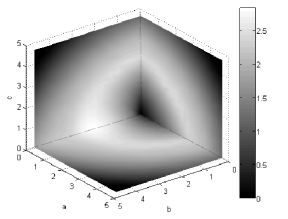
The method of discretization of Eqns (28), which are used to obtain the simulation results, will be described later in this article. Figure 1 indicates the slices along a quadrent of the co-ordinate axes of the actual minimum time function $C$ (which corresponds via Eq (27) to the normalized minimum function $S$, obtained by solving the HJB Eq (28)).

The figure is presented as a gray-scale image in a three dimensional grid. The axes correspond to the three parameters used for the representation of $SU(2)$ as described above. A lighter shading indicates a larger value of the minimum time function at a point, while a darker shading implies a smaller time to reach the identity element when starting from that point.

Figure 1: Un-normalized Optimal cost function with a control of norm 1

Figure 2: Path to the identity element starting at different points on each of the 3 axes.

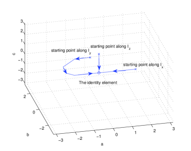
Time optimal trajectories for this example are indicated in Figure 2. Note that the non-uniqueness of the representation leads to having to carefully interpret the paths when they are shown in flat space. Observe that since there is no direct vector field to control along $I_{y}$, the path to the identity starting from a point along $I_{y}$ is not a straight line unlike in the case of the other two axes ($I_{x}$ and $I_{z}$).

The discretization of this system for obtaining numerical solutions to the HJB equation (28) is carried out using the finite difference procedure in (kushner2001nms, , Section 6.5). In three dimensional Euclidian space with a grid spacing $h$ of the space and basis vectors $e_{i}$, the value iteration equation (which is the iteration of the cost function, say $S^{h}$ ) is given by:

$${S^{h}}(x)=\mathop{\inf}\limits_{U}\left\{{\frac{h}{{h+\left\|f\right\|_{1}}}+\frac{{\sum\limits_{i=1}^{3}{{S^{h}}_{\pm}^{i}(x)\,f_{\pm}^{i}(x,U)}}}{{h+\left\|f\right\|_{1}}}}\right\},$$

where

$${S^{h}}_{\pm}^{i} :={S^{h}}(x\pm h\,e_{i})$$

$$f_{+}^{i}(x,U) :=\max\left\{{f^{i}(x,U),0}\right\}$$

$$f_{-}^{i}(x,U) :=-\min\left\{{f^{i}(x,U),0}\right\}$$

$$\left\|f(x)\right\|_{1} :=\sum\limits_{i=1}^{n}{\left\|f^{i}(x)\right\|}.$$ (30)

Here $f^{i}$ are the $i$ th components of the vector valued function $f$.

Note that the optimal control for this system is a specific case of Eq (18), where the possible values of the spatial co-ordinates are the locations of the grid points which in turn depend on the mesh generated for the discretization. These discretized equations and the controls resulting therefrom are used to obtain the simulation results indicated in the figures in this article. Once the controls are determined, we can generate the one and two qubit unitaries which efficiently approximate this control trajectory as explained in Section III.3.

V Discussion and conclusions

In this article we have described the use of the Dynamic programming method to solve the efficient gate synthesis problem and have demonstrated a proof of principle of this technique by obtaining a complete solution to an example problem of a single qubit.

A comparison between the method introduced and algebraic decomposition based approaches (such as applications of the methods in N.2001 ), is shown in sjcdc2008Underreview ; wherein it is demonstrated that the results obtained by a decomposition based method agree well, to within the error bounds of the discretization, with those resulting from the dynamic programming based control method.

The methods in the present article are sufficiently general to be able to be used with various cost functions such as the ones in schulteherbruggen2005ocb as well those used in geometric approaches to the problem as in Nielsen2006 .

The simulations in this work are based on theoretical results which are quite involved. A rigorous and complete development of the proofs of the foundations of this article will be deferred to a future publication. The numerical procedures outlined herein generalize to higher dimensional cases with the crucial limiting factor being the time taken and storage requirements for these computations (which increases dramatically with the dimension of the system). The treatment of problems of direct interest to gate complexity will require an analysis of unitaries on three or more qubits. Owing to the curse of dimensionality, further work is required to develop computational methods of greater efficiency in order to use the Dynamic Programming technique to investigate these problems of practical interest.