Pion LINAC as an Energy-Tagged $\nu$ Source

Abstract

The energy spectrum and flux of neutrinos from a linear pion accelerator are calculated analytically under the assumption of a uniform accelerating gradient. The energy of a neutrino from this source reacting in a detector can be determined from timing and event position information.

I Introduction

There has been considerable analysis FNAL of the value of a high energy muon storage ring for the purpose of producing well-defined, high energy beams of neutrinos. This approach takes advantage of the relatively long muon lifetime to allow for collection at modest energies and acceleration to very high energies, where the decay neutrinos form an intense, highly collimated beam. The proposals for such systems are quite expensive since the (generally hadronically) produced muons must be captured, cooled and accelerated, all on a microsecond time scale.

Some time ago, Los Alamos proposed PILAC a pion post-accelerator (PILAC) to be appended to the then extant meson factory, LAMPF. The proposal took advantage of the high pion flux produced at modest energies, to collimate and inject into a high gradient linac. Phase rotation was introduced to reduce the energy spread of the beam considerably. The main practical difficulty with this relatively modest cost proposal was the short pion lifetime – 26 nanoseconds. This required a very high accelerating gradient in order to achieve a useable flux at the exit of the acceleration section.

The decay of a positively-charged pion is almost exclusively into anti-muons and muon-neutrinos (or muons and muon-antineutrinos for negatively-charged pions) with a purity at the part in ten thousand level. Thus a PILAC also provides an intense, collimated beam of neutrinos with an energy spectrum ranging from negligible to initially half the pion input energy and finally to half the output energy value. We show here that the neutrino spectrum, $dN_{\nu}/dE_{\nu}$, can adjusted to be almost flat in energy, if sufficiently high accelerating gradients for the pions can be achieved. The necessary values are below those already achieved LEP using superconducting RF cavities.ftn1

However, there is another advantage to such a neutrino source that does not dependent upon whether or not high gradients can be achieved. Currently, it is very difficult to determine the energy of the neutrino involved in a particular scattering event in the detector. Usually, a complicated series of Monte Carlo simulations of the detector and its response defines a statistical determination only. In the scheme we are discussing, however, it is possible to obtain the incident neutrino energy directly, event by event.

We analyze here the theoretically simple case of a uniform accelerating gradient analytically. A more realistic case with drift sections is left for the accelerator physicists who would actually design and build such a system.

II Calculations

Although we ultimately want to obtain the neutrino energy spectrum as a function of distance from the injection point of the accelerator, to follow the decay rate, it turns out to be more convenient to first find the pion energy and decay rate as functions of time. Throughout, we will use units where $\hbar=c=1$.

II.1 Time Dependence

We begin with pions injected at energy $E_{I}$ and $\gamma_{I}\equiv E_{I}/m_{\pi}$ where $m_{\pi}$ is the pion mass. For simplicity, we assume a spatially constant, uniform accelerating gradient, $G$, even though the actual acceleration structure will consist of short, high acceleration regions interspersed with drift regions. Refinement to include this detail should only change our smooth curves to segments of alternating flat and higher slope regions but with essentially the same average behavior. For convenience, we scale $G$ by the pion mass so that $g\equiv G/m_{\pi}$ has the dimensions of an inverse length,

$$gm_{\pi}=dE_{\pi}/dx\ .$$ (1)

The energy of a pion as a function of distance along the accelerator is therefore

$$E_{\pi}(x)=E_{I}+gm_{\pi}x\ .$$ (2)

However, to follow the decay process, we will need the time rate of change of pion energy, viz.,

$$dE_{\pi}/dt=\frac{dE_{\pi}}{dx}\frac{dx}{dt}=gm_{\pi}\beta(t)\ ,$$ (3)

where $\beta(t)$ is the pion velocity in units of $c$. Since $\gamma(t)=E_{\pi}/m_{\pi}$, we can rewrite Eq. (1) as

$$d\gamma/dt=g\beta$$ (4)

and since $\gamma=1/\sqrt{1-\beta^{2}}$,

$$\frac{d\gamma}{dt}=\frac{\beta}{[1-{\beta}^{2}]^{\;3/2}}\frac{d\beta}{dt}\ .$$ (5)

Eq. (4) thus becomes

$$\frac{1}{[1-{\beta}^{2}]^{\;3/2}}\frac{d\beta}{dt}=g\ .$$ (6)

This is easily integrated to obtain

$$\frac{\beta(t)}{[1-{\beta}^{2}(t)]^{1/2}}=gt+\frac{\beta(0)}{[1-{\beta}^{2}(0)]^{1/2}}\ ,$$ (7)

or equivalently,

$$\beta(t)\gamma(t)=gt+\beta(0)\gamma(0)\equiv gt+\alpha_{0}\ .$$ (8)

This allows us to identify

$$\beta(t) = \frac{gt+\alpha_{0}}{\sqrt{1+({gt+\alpha_{0}})^{2}}}\ ,$$ (9)

$$\gamma(t) = \sqrt{1+({gt+\alpha_{0}})^{2}}\ .$$ (10)

Bear in mind that $\alpha_{0}$ is implicitly a function of the injected pion energy. Eq. (8) is just the well-known result that a constant accelerating energy gradient causes the momentum to increase linearly with time, i.e., $p(t)=m_{\pi}gt+p_{I}$, where $p_{I}=m_{\pi}\alpha_{0}$ is the pion momentum at injection into the accelerator.

II.2 Decay

With $\gamma(t)$ in hand, we can solve for the pion decay function in the rest frame of the accelerator, viz.

$$\frac{dN_{\pi}}{dt}=-\frac{\Gamma}{\gamma(t)}N_{\pi}(t)=-\;\frac{\Gamma}{\sqrt{1+(gt+\alpha_{0})^{2}}}N_{\pi}(t)\ ,$$ (11)

where $\Gamma$ is the decay rate of the pion in its own rest frame. Integration of this equation yields

$$N_{\pi}(t)=N_{\pi}(0)\left[\frac{(gt+\alpha_{0})+\sqrt{1+(gt+\alpha_{0})^{2}}}{\alpha_{0}+\sqrt{1+\alpha_{0}^{2}}}\right]^{-\Gamma/g}\ .$$ (12)

Since the number of neutrinos is just equal to the number of pions that have decayed, $N_{\nu}(t)=N_{\pi}(0)-N_{\pi}(t)$, it follows immediately that

$$N_{\nu}(t)=N_{\pi}(0)\left(1-\left[\frac{\alpha_{0}+\sqrt{1+\alpha_{0}^{2}}}{(gt+\alpha_{0})+\sqrt{1+(gt+\alpha_{0})^{2}}}\right]^{\Gamma/g}\right)\ .$$ (13)

II.3 Distance Dependence

We next convert this time dependence into spatial dependence, as a function of distance from the input of the linear accelerator. We can integrate $\beta=dx/dt$ given by Eq. (9) to obtain

$$x(t)=\int_{0}^{t}dt^{\prime}\beta(t^{\prime})=\frac{\sqrt{1+(gt+\alpha_{0})^{2}}-\sqrt{1+\alpha_{0}^{2}}}{g}\ ,$$ (14)

where we chose $x(0)=0$. Eq. (14) can easily be inverted to obtain

$$t(x)=\frac{[(gx+\gamma(0))^{2}-1]^{1/2}-\alpha_{0}}{gc}\ ,$$ (15)

and this may be substituted into Eq. (13) to obtain $N_{\nu}(x)$. Our result for the neutrino flux at a distance $x$ is, therefore,

$$N_{\nu}(x)=N_{\pi}(0)\left[1-\left(\frac{\alpha_{0}+\sqrt{1+\alpha_{0}^{2}}}{gx+\sqrt{1+\alpha_{0}^{2}}+[(gx+\sqrt{1+\alpha_{0}^{2}}\;)^{2}-1\;]^{1/2}}\right)^{\Gamma/g}\right].$$ (16)

Noting that $m_{\pi}\sqrt{1+\alpha_{0}^{2}}=E_{I}$, we convert this back to the original variables,

$$N_{\nu}(x) = N_{\pi}(0)\left[1-\left(\frac{p_{I}+E_{I}}{gm_{\pi}x+E_{I}+\sqrt{[gm_{\pi}x+E_{I}]^{2}-m_{\pi}^{2}}}\right)^{\Gamma/g}\right]$$ (17)

$$= N_{\pi}(0)\left[1-\left(\frac{E_{I}+p_{I}}{E_{x}+p_{x}}\right)^{m\Gamma/G}\right]\ ,$$

where $E_{x}$ and $p_{x}$ are the energy and momentum of the pion after travelling a distance $x$ through the accelerator.

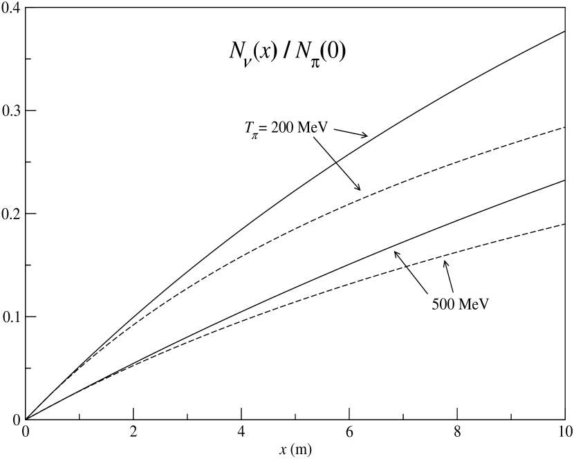
Figure 1: Dependence of $N_{\nu}(x)$, normalized by the number of input pions, $N_{\pi}(0)$, as a function of distance along the pion accelerator, $x$, for two pion kinetic energies spanning the production peak at injection into the accelerator. The solid curves are for a gradient of 10 MeV/m, while the dashed curves are for 50 MeV/m.

Fig. 1 shows the behavior of $N_{\nu}(x)$ for two different accelerating gradients and for two different initial pion kinetic energies (in the laboratory). As expected, the $x$-dependence becomes more and more linear as the injection energy increases. Also, the higher the gradient, the flatter the curves become. The reason for this is that a bigger gradient means higher energy pions, which have longer lifetimes (in the laboratory), whence fewer decays into neutrinos during acceleration.

The accelerator designer may therefore want to optimize between the number of neutrinos showing up in the detector (normalized by the number of pions captured in the accelerator) and their ultimate energies. One might also want to consider the possibility of making a pion de-celerator, if it turns out that lower energy neutrinos have desirable properties for some experiments.

II.4 Neutrino Energy Spectrum and Angular Divergence

The neutrino energies will range over a wide spectrum, but for any specific time from injection of the pion bunch and angle of divergence from the beam axis of a neutrino scattering event in the detector, only one specific neutrino energy is possible.

The momentum and energy, $E_{0}$, of a neutrino emitted in the pion rest frame is

$$E_{0}=\frac{m_{\pi}^{2}-m_{\mu}^{2}}{2m_{\pi}}=29.8{\rm\ MeV}\ .$$ (18)

For a decay where the neutrino is emitted at a polar angle $\theta_{R}$ (in the rest frame) with respect to the pion beam axis, the momentum, polar angle $\theta_{L}$, and energy $E_{\nu}$ in the lab frame are given by

$${\bf p} = E_{0}\;[\gamma(\beta+\cos\theta_{R}),\;\sin\theta_{R}]\ ,$$ (19)

$$\tan\theta_{L} = \sin\theta_{R}/[\gamma(\beta+\cos\theta_{R})]\ ,$$ (20)

$$E_{\nu} = E_{0}\;\sqrt{\sin^{2}\!\theta_{R}+\gamma^{2}(\beta+\cos\theta_{R})^{2}}$$ (21)

$$= \gamma(1+\beta\cos\theta_{R})E_{0}\ ,$$

where we show only the longitudinal and transverse momentum components, ignoring the azimuthal angle since the distribution in that angle is uniform.

From Eq. (21), neutrinos emitted exactly backward from the beam direction will have lab energies and momenta of $\gamma(1-\beta)\;E_{0}$, i.e., approximately zero for the most relativistic pions. Those emitted precisely forward will have lab energies and momenta of $\gamma(1+\beta)\;E_{0}$. For neutrinos emitted transverse (in the pion rest frame) to the beam direction, the lab energy and momentum will be $\gamma E_{0}$.

From Eq. (20), the singularity at $\cos\theta_{R}=-\beta$ corresponds to a laboratory angle of 90^∘. Neutrinos at this angle come from a very backward decay and have a low energy of $E_{0}/\gamma$. Those that come from even more backward decays have yet lower energies. The maximum laboratory angle is 180^∘. That is, $\theta_{L}$ as a function of $\theta_{R}$ rises monotonically from 0 to 180^∘, and does so more steeply in the backward $\theta_{R}$ direction.

Neutrinos are emitted between the two extreme energies along a curve in $E_{\nu}$-$\theta_{L}$ space. To make such a plot, one needs to find the value of $\cos\theta_{R}$ corresponding to a given laboratory angle, $\theta_{L}$. From the inverse Lorentz transformation, from the laboratory to the pion rest frame, and with some algebra,

$$\cos\theta_{R}=\cos\left[\tan^{-1}\left(\frac{\sin\theta_{L}}{\gamma(\cos\theta_{L}-\beta)}\right)\right]=\frac{\cos\theta_{L}-\beta}{1-\beta\cos\theta_{L}}\ .$$ (22)

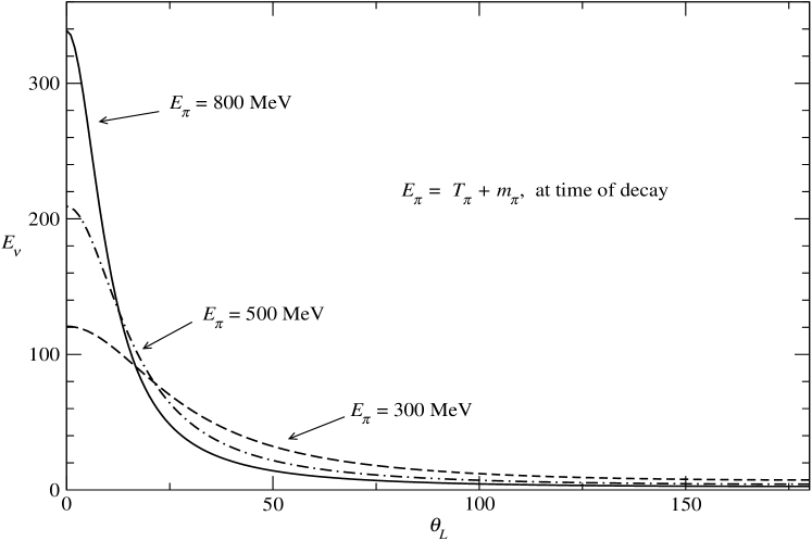
Figure 2: The neutrino energy, $E_{\nu}$ (in MeV), as a function of laboratory polar angle $\theta_{L}$ from decay in the acceleration section at a given time from bunch injection (or position in the accelerator) for three pion kinetic energies at the time of decay. Each pion energy corresponds to a specific location for the decay in the accelerator section.

Having found the value of $\cos\theta_{R}$ for a given (or derived) $\theta_{L}$, the neutrino energy $E_{\nu}$ is then given by Eq. (21), or more directly, $E_{\nu}=(1-\beta\cos\theta_{L})^{-1}E_{0}/\gamma$. Figure 2 shows curves of the neutrino energy as a function of $\theta_{L}$ for three different (total) energies of the pion at the time of its decay. Note that, for the higher pion energies, the neutrino energy $E_{\nu}$ is more forward peaked and, of course, is larger there. Taking into account that neutrino cross sections are proportional to $E_{\nu}^{\ 2}$ at low $E_{\nu}$, this suggests that, for economy, the neutrino detector could well be long and narrow, subtending a small solid angle along the beam direction.

II.5 Determining $E_{\nu}$ From Event Timing

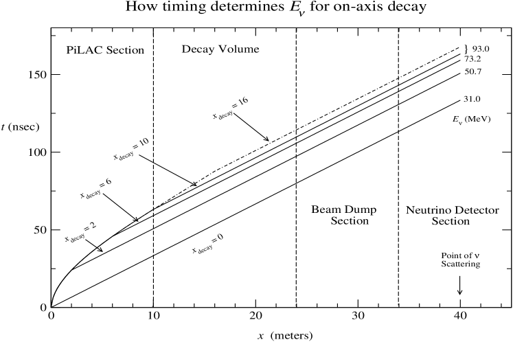
Figure 3: Relation between decay time after pion bunch injection and time of scattering event in detector for on-axis $\nu$’s of the highest energy. This is for an unrealistic injection energy of $T_{\pi}$ = 100 keV, so that the curvatures before decay are highly exaggerated.

Fig. 3 depicts an example of what we have in mind, a pion accelerator which is 10 m long.ftn2 This is followed by an air-filled drift space (i.e., a decay volume) of 14 m, a 10 m long beam dump, such as earth or iron, and the neutrino detector, presumed, for cost-effectiveness, to be a long cylinder aligned with the beam axis.ftn3 The drift space could also provide space for experiments using the pions which emerge from the accelerator. It also might contain bending magnets to deflect charged particles from the beam axis.ftn4

Neutrinos all travel at velocity $c$, which is discernably larger than the velocity of the pions (up to $\approx$ 1 GeV pion energy). Thus the time of scattering and the position of the event in the detector are uniquely correlated (up to resolution limits) with the energy of the neutrino. However, low-energy neutrino cross sections vary as $E_{\nu}^{2}$, so most of the neutrino events will come at forward angles less than $\approx 30^{\circ}$.

We discuss first the case for those higher-energy neutrinos emitted at $0^{\circ}$ along the beam direction. Fig. 3 shows how the change in pion velocity along the accelerator, followed by speed-of-light propagation of the neutrino from the decay point, determines the neutrino energy. Note that this figure is for an unrealistic injection energy of $T_{\pi}$ = 100 keV, simply to show the principle involved.ftn5 The idea is to measure the difference between the time when the neutrino scattering event occurs and that for a light-like signal that begins at the time the pions are injected into the pion accelerator. The neutrino energy $E_{\nu}$ in this on-axis case is given by

$$E_{\nu,\;{\rm on-axis}}=\gamma(t_{\rm dec})\;[1+\beta(t_{\rm dec})]\;E_{0}\ ,$$ (23)

where $t_{\rm dec}=t(x_{\rm dec})$ is given by Eq. (15) and $E_{0}$ by Eq. (18). The value of $x_{\rm dec}$ needed for $t_{\rm dec}$ is obtained by solving the more general expression for the event time, Eq. (24), given below.

Note also that some pions will decay after leaving the accelerator. In such cases, as in the dot-dashed curve in Fig. 3, the timing for the event will be later than the case shown when $x_{\rm decay}$ = 10 m, but $E_{\nu}$ will be the same, i.e., 93.0 MeV in this example.

For more realistic injection energies, e.g., $T_{\pi}$ = 350 MeV, the curves in the pion accelerator section are much, much flatter than those shown in Fig. 3. The time differences are quite small but technically feasible.

$x_{\rm decay}$ (m)	$G$ = 10 MeV/m		$G$ = 50 MeV/m
	$\Delta t$ (nsec)	$E_{\nu}$ (MeV)	$\Delta t$ (nsec)	$E_{\nu}$ (MeV)
0.0	0.000	205	0.000	205
2.0	0.275	214	0.236	249
4.0	0.528	223	0.401	292
6.0	0.762	231	0.522	335
8.0	0.978	240	0.616	379
10.0	1.179	249	0.691	422

Table 1: The calculations shown here are for $T_{\pi}$ = 350 MeV at injection into PILAC.

For an injection energy of $T_{\pi}$ = 350 MeV, Table I shows, for two choices of accelerating gradient $G$, the time differences, in nanoseconds, and the higher-energy neutrinos’ associated energies. Note that, to distinguish the two highest energies shown for $G=$ 50 MeV/m, one must have timing resolution of about 50 picoseconds.

A similar but more complicated relation occurs for radially off-axis points, where the decay angle must be included in the correlation. (See Fig. 2.) The procedure for determining $E_{\nu}$ from the time the event occurs (relative to the time of injection of the pions into the accelerator) is as follows.

If the position of the event in the detector is given by $(x_{\rm evt},\rho_{\rm evt})$, where $x_{\rm evt}$ is measured from the injection point and $\rho_{\rm evt}$ is the transverse distance from the beam axis, the time of the event is

$$t_{\rm evt}(x_{\rm dec},x_{\rm evt},\rho_{\rm evt})=t_{\rm dec}(x_{\rm dec})+t_{\nu}(x_{\rm evt}-x_{\rm dec},\rho_{\rm evt})\ ,$$ (24)

where $t_{\rm dec}(x)$ is given by Eq. (15) and $t_{\nu}(x,\rho)=\sqrt{x^{2}+\rho^{2}}/c$. Equation (24) can be solved numerically for $x_{\rm dec}$. The implicit dependence in $t_{\rm dec}$ on the gradient, $G$, and the kinetic energy $T_{\pi}$ of the injected pions should be kept in mind.

Given the extracted value for $x_{\rm dec}$, we can infer that the neutrino was emitted at a laboratory angle of

$$\theta_{L}=\tan^{-1}[\rho_{\rm evt}/(x_{\rm evt}-x_{\rm dec})]\ .$$ (25)

The pion energy at the time it decays is also determined by $x_{\rm dec}$. From Eqs. (10) and (15),

$$\gamma_{\rm dec} = \sqrt{1+[gt(x_{\rm dec})+\alpha_{0}]^{2}}\ ,$$ (26)

$$\beta_{\rm dec} = \sqrt{\gamma_{\rm dec}^{2}-1}\;/\gamma_{\rm dec}\ ,$$ (27)

$$E_{\pi} = m_{\pi}\;\gamma_{\rm dec}\ .$$ (28)

From the values of $\theta_{L}$, $\beta_{\rm dec}$, and $\gamma_{\rm dec}$ the cosine of the decay angle in the pion rest frame is then found by substituting these values into Eq. (22):

$$\cos\theta_{R}=\frac{\cos\theta_{L}-\beta_{\rm dec}}{1-\beta_{\rm dec}\cos\theta_{L}}\ .$$ (29)

The neutrino energy $E_{\nu}$ is then determined by substituting this value of $\cos\theta_{R}$ into Eq. (21).

		$G$ = 10 MeV/m			$G$ = 50 MeV/m
$\Delta t$ (nsec)	$\ \rho_{\rm evt}\$	$x_{\rm dec}$	$\ \theta_{L}\$	$E_{\nu}$	$x_{\rm dec}$	$\ \theta_{L}\$	$E_{\nu}$
0.250	0.3	1.81	7.9	213	2.15	7.9	252
	0.6	1.72	15.7	213	2.02	15.8	249
	0.9	1.58	23.4	212	1.82	23.6	245
0.500	0.3	3.77	8.3	222	5.58	8.7	327
	0.6	3.67	16.5	221	5.35	17.3	322
	0.9	3.50	24.7	221	4.99	25.7	314
0.750	0.3	5.89	8.9	231	11.9	10.7	463
	0.6	5.77	17.5	231	11.3	20.9	450
	0.9	5.58	26.1	230	10.5	30.6	433

Table 2: Extractions of the decay point $x_{\rm dec}$ (in m), neutrino laboratory angle $\theta_{L}$ (in mrad), and $E_{\nu}$ (in MeV) for a scattering event taking place at various scattering times $\Delta t$ in the detector at three values of off-axis radial position $\rho_{\rm evt}$. This case is for an event occurring in the detector at $x_{\rm evt}$ = 40.0 m from the accelerator injection point. We have assumed here that $T_{\pi}$ = 350 MeV at injection into PILAC, as in Table I.

Table II shows the correlations between measured scattering times $\Delta t$ and off-axis event positions $\rho_{\rm evt}$ and the extracted values for the decay point $x_{\rm dec}$, laboratory neutrino angle $\theta_{L}$, and $E_{\nu}$, for the same two accelerating gradients and injection energy used in Table I. Because of the small solid angle subtended by the detector, in this example, the time differences at off-axis points are not much different from those shown in Table I. Thus transverse spatial resolution becomes a significant contributor to determination of the neutrino energy, implicitly demanding a fine-grained detector.

Fig. 4 illustrates the correlation for an off-axis detection of a neutrino between the time of the event and the pion decay point and angle of decay (as seen in the lab frame), whence the energy of the reacting neutrino.

III Discussion

Note that, as shown by Eq. (17), the important scale for the acceleration gradient is set by the lifetime of the pion in units of pion mass, namely,

$$G=m_{\pi}\Gamma_{\pi}/c=17.9\;{\rm MeV/m}\ .$$ (30)

Gradients exceeding this value are now routinely available, which makes possible very tightly focussed neutrino beams and unusual neutrino energy spectral distributions.

The higher the gradient can be made, the more pions survive to the exit energy and the neutrino spectrum becomes more and more weighted to higher energies. The higher energy component of the neutrino beam also becomes more focused, projecting a smaller image on the target.

The pion particle flux expected from the design in Ref. PILAC was $10^{9}s^{-1}$ at the target end of the accelerator. With the gradient given above, the accelerator would be on the order of 5 lifetimes in length. Thus, while the neutrino flux at the highest energy available would be on the order of $10^{9}s^{-1}$, the total flux over the entire spectrum would be on the order of $10^{11}s^{-1}$ (since nearly every injected pion will decay into a neutrino). This certainly presents a challenge to experimenters to design detectors with a useful event rate, as the flux is not as large as produced by simple beam target-decay volume sources.

An additional order of magnitude in flux should be available if the PILAC system were to be mounted at the Spallation Neutron Source at Oak Ridge National Laboratory.

We thank J. Jenkins, W. Louis, G. Mills, and C. Morris for valuable conversations. This work was carried out under the auspices of the National Nuclear Security Administration of the U.S. Department of Energy at Los Alamos National Laboratory under Contract No. DE-AC52-06NA25396

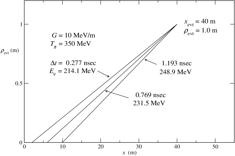
Figure 4: Relation between the reacting neutrino’s energy, $E_{\nu}$, and the time difference between the time of bunch injection and the scattering event time in the detector for a particular event position, here at 40 meters from the start of the pion accelerator and at an off-axis distance of 1 meter. It shows the differences in $E_{\nu}$ and time difference $\Delta t$ for three different pion decay positions. The kinetic energy of pions at injection has been taken to be 350 MeV and the accelerating gradient is 10 MeV/m. Thus, in this example, if the absolute time of this scattering event can be determined relative to the injection time with an accuracy of better than $\sim 500$ ps, then the energy of the incident neutrino that initiated the event will be determined to an accuracy of better than $\approx 15$ MeV.

References

- (1) S. Geer, Phys. Rev. D57 (1998) 6989. Subsequent development of the neutrino factory idea includes work, for example, by A. Bandyopadhyay et. al., arXiv:0710.4947 and by C. H. Albright et al., arXiv/physics/0411123. See also references therein.
- (2) “Overview of the PILAC project”, Barbara Blind, Report No. LA-UR-04-3797, provides a useful, brief synopsis. Earlier published work includes H. A. Thiessen and D. Hywel White, Zeit. f. Phys. C. 56, 285 (1992); H. A. Thiessen, Nucl. Phys. A 547, 339 (1991); B. Blind, Particle Accelerator Conference, 1991, pp. 899-901; S. Nath, G. Swain, R. Garnett, and T. P. Wangler, OSTI 6541038, 1990.
- (3) See, e.g., B. Aune et al., “Superconducting TESLA cavities”, Phys. Rev. ST Accel. Beams 3 (2000) 092001; W.D. Moeller, “The Performance of the 1.3 GHz Superconducting RF Cavities in the First Module of the TESLA Test Facility Line, XIX International Linear Accelerator Conference, Chicago, Illinois, USA August 23 - 28, 1998; M. Ono et al., “Achievement of 40 MV/m Accelerating Field in L-Band SCC at KEK”, in Proc. of the 8th RF Superconducting Workshop, Padova, 1997.
- (4) In the examples given in the tables below, we will use two values of gradients, 10 MeV/m and 50 MeV/m. The latter value is rather speculative, but might be achievable in the future. In this regard, for a F0D0 linac rather than the continuous gradient design we assume here (for simplicity of presentation), the average gradient will be less than that of a given RF cavity. Also, the gradient achievable could depend upon on aperture required to match the emittance of the pion beam being accelerated. Our only intention, in showing the 50 MeV/m case, is to indicate the effects of achieving high gradients. As noted in the introduction, even at lower gradients, the design has a significant value in affording the determination of the energy of the incident neutrino event by event.
- (5) The PILAC design PILAC was for a rather longer accelerator, 102.9 m, but this was to get the highest possible energies for the pions. Also, the accelerating gradient in that design was only 12.5 MeV/m, befitting the technology available at that time.
- (6) Any realistic detector proposal could only be made after a realistic accelerator design has been developed. Our hope is that a highly instrumented device, long but with a relatively small transverse size, might be feasible.
- (7) Without such a bend, muons from pion decays might otherwise penetrate the beam dump and give background events in the neutrino detector which follows. The background from neutrons in the beam direction should be small. Note that the injection “snake” severely limits the pions in the linac in both momentum and charge, so opposite-sign pions and muons should be totally negligible.
- (8) Details dependent on realistic beam dispersion and timing errors will blur these lines.