Simulations of the formation and evolution of isolated dwarf galaxies

Abstract

We present new fully self-consistent models of the formation and evolution of isolated dwarf galaxies. We have used the publicly available N-body/SPH code HYDRA, to which we have added a set of star formation criteria, and prescriptions for chemical enrichment (taking into account contributions from both SNIa and SNII), supernova feedback, and gas cooling. We extensively tested the soundness of these prescriptions and the numerical convergence of the models. The models follow the evolution of an initially homogeneous gas cloud collapsing in a pre-existing dark-matter halo. These simplified initial conditions are supported by the merger trees of isolated dwarf galaxies extracted from the milli-Millennium Simulation. The star-formation histories of the model galaxies exhibit burst-like behaviour. These bursts are a consequence of the blow-out and subsequent in-fall of gas. The amount of gas that leaves the galaxy for good is found to be small, in absolute numbers, ranging between $3\times 10^{7}\ M_{\sun}$ and $6\times 10^{7}\ M_{\sun}$. For the least massive models, however, this is over 80 per cent of their initial gas mass. The local fluctuations in gas density are strong enough to trigger star-bursts in the massive models, or to inhibit anything more than small residual star formation for the less massive models. Between these star-bursts there can be time intervals of several Gyrs.

The models’ surface brightness profiles are well fitted by Sérsic profiles and the correlations between the models’ Sérsic parameters and luminosity agree with the observations. We have also compared model predictions for the half-light radius $R_{\mathrm{e}}$ , central velocity dispersion $\sigma_{\mathrm{c}}$, broad band colour $B-V$, metallicity $[Z/Z_{\sun}]$ versus luminosity relations and for the location relative to the fundamental plane with the available data. The properties of the model dwarf galaxies agree quite well with those of observed dwarf galaxies. However, the properties of the most massive models deviate from those of observed galaxies. This most likely signals that galaxy mergers are starting to affect the galaxies’ star-formation histories in this mass regime ($M\gtrsim 10^{9}\ M_{\sun}$).

We found that a good way to assess the soundness of models is provided by the combination of $R_{\mathrm{e}}$ and $\sigma_{\mathrm{c}}$. The demand that these are reproduced simultaneously places a stringent constraint on the spatial distribution of star formation and on the shape and extent of the dark matter halo relative to that of the stars.

1 Introduction

Dwarf galaxies (DGs), galaxies with blue absolute magnitude $-14>M_{\mathrm{B}}>-18$ mag, are the most numerous type of galaxies in the nearby universe (Ferguson & Binggeli, 1994). Besides their number there are various reasons why DGs are very important in modern astronomy, most notably their cosmological relevance.

In the Lambda cold dark matter ($\Lambda$CDM) cosmological model, present day galaxies are the product of a series of mergers. The early universe consisted of a uniform density, superimposed with small Gaussian fluctuations. As their amplitude increases monotonically toward smaller scales, they give, after inflation, rise to a myriad of small virialized dark matter (DM) haloes. These small haloes collapse first under influence of their own gravity, followed by the collapse of haloes with larger masses, swallowing the smaller haloes. We thus have hierarchical clustering, where massive galaxies, such as our own Milky Way, have formed through the merger of DGs. Dwarf galaxies are therefore an important link in the chain of hierarchical clustering. Moreover due to their relatively low total mass ($\mathcal{O}(10^{7}-10^{9}\ M_{\sun}$)) they are quite sensitive to the effects of gravitational interactions, star formation (SF) and supernova (SN) explosions. On the one hand DGs are therefore the ideal objects to study when researching SF and SNe in a galaxy environment, and dynamical evolution of galaxies in general. Understanding the birth and life of DGs on the other hand could prove crucial when trying to understand the formation and evolution of more massive stellar systems. And even more: cosmological simulations of galaxy formation exhibit very strong dependence on the way star formation, feedback (FB) through supernovae and stellar winds (SW) are modelled within stellar systems (see e.g. White & Frenk, 1991; Kauffmann et al., 1999). Therefore realistic simulations of single dwarf galaxies can supply information on how to implement star formation and feedback processes in large cosmological simulations (e.g. Springel et al., 2005), where a fully consistent implementation of SF and FB should be possible for moderate simulation volumes.

From the theoretical point of view various approaches for the study of DGs are possible, most notably there are semi-analytical models (SAMs), consisting of a limited set of analytical equations solved numerically, and fully numerical simulations, Lagrangian (e.g. N–body/SPH) or Eulerian (grid codes). SAMs have the advantage of computational efficiency, due to their speed it is possible to scan a large part of the parameter space in a reasonable period of time. In numerical simulations however a fully self consistent implementation of SF, FB, chemical enrichment, gas cooling, … is possible, at the price of high computational effort.

Dekel & Silk (1986) were the first to model Dwarf Galaxies (DGs), emphasising the impact of supernova-driven winds on the formation of dwarfs. Yoshii & Arimoto (1987) found good agreement between observational properties of DGs and those predicted by their SAM. These authors calculated the properties of DGs (and globular clusters), using a model that takes into account the dynamical response to a supernova-driven wind. An evolutionary population synthesis method is employed to bring the models into the observational domain. According to these models, spheroidal galaxies are a one-parameter family of birth mass (initial total mass $M_{\mathrm{t,i}}$). These models were later extended in Nagashima & Yoshii (2004), who used a Monte Carlo technique to construct the merger tree leading up to the formation of a DG. Nagashima et al. (2005) incorporated N–body simulations instead of a Monte Carlo method to construct the merger tree. They found good agreement between galaxies produced by their SAM, ranging from dwarf elliptical to elliptical galaxies, and observations. SAMs are also used to investigate certain processes involved in the birth and life of dwarf galaxies rather than trying to reproduce dwarf galaxies, e.g. the model of Burkert & Ruiz-Lapuente (1997), investigating the role of SNIa in delaying star formation and of Ferrara & Tolstoy (2000) who investigated the role of stellar feedback and dark matter.

Although plenty of numerical research has already been carried out concerning the formation and evolution of massive elliptical galaxies (EG) (to name a few: Katz, 1991; Kawata, 2001; Chiosi & Carraro, 2002; Kawata & Gibson, 2003; Kobayashi, 2005; Merlin & Chiosi, 2006), starting from various cosmological initial conditions, only few people have tried directly modelling DGs with fully numerical simulations. One problem is that DGs are too small to be adequately resolved in large cosmological simulations. A first fully numerical study of dwarfs was performed by Mori et al. (1997); Mori et al. (1999), who explored the role of gas cooling in dwarf galaxy formation. Chiosi & Carraro (2002) used an N–body/SPH code to simulate the formation of galaxies, including dwarf spheroidal, dwarf elliptical and normal elliptical galaxies. They started from cosmologically inspired initial conditions. Assuming that star formation starts after an initial merging period, the simulations start with the collapse of an initially homogeneous gas cloud in a dark matter halo (White & Rees, 1978). Observable properties of DGs were broadly reproduced by their models. More recently, Stinson et al. (2007) conducted simulations of dwarf spheroidal galaxies (dSph). They used initial conditions similar to those of Chiosi & Carraro (2002), except that a degree of rotation was added to the gas. Like Chiosi & Carraro (2002), these authors find burst-like star formation. The work of Stinson et al. (2007) is based on the work by Stinson et al. (2006), who investigated the influence of star formation criteria on the formation of a galaxy, as well as the dependence of the processes involved on the number of particles. Mashchenko et al. (2007) performed fully cosmological simulations of the formation of a few dwarf galaxies, focusing on the gravitational heating of the dark matter, induced by gas flows. They argue that this heating can effectively convert a cusped dark matter halo into a DM halo with a central core. Other studies of dSphs include those of Read & Gilmore (2005), who looked at the effect of baryonic mass loss from a two component galaxy (dark and baryonic matter) and Read et al. (2006), who used cosmological simulations to investigate the smallest baryonic building blocks for galaxy formation. Mashchenko et al. (2005) employed a simple model for the formation of dwarf spheroidal galaxies. A single star-burst was imposed on a gas distribution, employing a density cutoff, after which the remaining gas was removed. They find reasonable agreement with data from local group dwarf spheroidal galaxies.

A study of dwarf galaxies in a cosmological context was performed by Scannapieco et al. (2001), investigating the effect of gas outflows on the formation of dwarf galaxies. Other studies using simulations, not directly aimed at reproducing dwarf galaxies, include those of Mac Low & Ferrara (1999), who used a two-dimensional grid code to model blowout/blow-away of gas in dwarf galaxies, and more recently Marcolini et al. (2006), who used a three-dimensional grid code to study the ISM in dwarf spheroidal galaxies by imposing a burst-like Star formation history (SFH) and comparing the results to the Draco dSph.

In this paper we present the results of our models of dwarf galaxies, with initial conditions taken from the $\Lambda$CDM formalism. As we construct spheroidal, non-rotating galaxies, we expect them to resemble dwarf spheroidal and dwarf elliptical galaxies. We took great care to avoid the introduction of a direct dependence on the number of particles or on the resolution into the formalism. We also investigate the role of the different star formation criteria in detail. We then compare our model data to observations using the central velocity dispersion, the half-light radius, $B-V$ broad band colours, total metallicity and the fundamental plane.

The outline of this paper is as follows. In § 2, we summarise the most important features of the modelling code. The initial conditions of our models are discussed in § 3. In § 4, we compare our models with observational data. We end with a summary and our conclusions in § 5.

2 The Code

We constructed our models using the N–body/SPH code HYDRA (Couchman et al., 1995; Thacker et al., 2000). In an N–body/SPH code the gravitational equations are solved with an N–body integrator. Hydrodynamical forces are applied through a Smoothed Particle Hydrodynamics (SPH) formalism (Lucy, 1977; Gingold & Monaghan, 1977). In this formalism the density at the position of the $i$-th (gas) particle is:

$$\rho_{\mathrm{g},i}=\sum_{j\neq i}m_{j}W(r_{ij},h_{i}),$$ (1)

where $r_{ij}=|\vec{r}_{i}-\vec{r}_{j}|$, $h_{i}$ is the smoothing length of the $i$-th particle and $W$ is the smoothing kernel. The use of the SPH formalism lies in the fact that derivatives of e.g. $\rho_{\mathrm{g}}$ can be expressed as derivatives of the smoothing kernel $W$. HYDRA was modified by us to include star formation, feedback, chemical enrichment, radiative cooling and supernovae (type II and Ia).

2.1 Star formation

To implement star formation in our code we use a phenomenological, Lagrangian approach. The first step is to formulate a set of star formation criteria.

2.1.1 Star Formation Criteria

We strive to select a set of Star-Formation Criteria (SFC) that allows our simulations to mimic real-life star formation. A number of implementations is compared in Kay et al. (2002), who find that different implementations of SF give comparable results. We will use a variant of the Katz et al. (1996) criteria, where it is assumed that star formation takes place in cool, dense, converging and gravitationally unstable molecular clouds. A good review of these criteria is given by Stinson et al. (2006). We select cool, dense and converging clouds in a very straightforward manner: the temperature of gas eligible for star formation must be lower than a certain critical temperature $T_{\mathrm{c}}=15\,000\ \mathrm{K}$ (Stinson et al., 2006, 2007). The density of a star forming gas cloud must exceed a critical density $\rho_{\mathrm{g}}=2\times 10^{-25}$ g cm-3, $n_{\mathrm{H}}\approx 0.1\ \mathrm{cm-3}$ (Kawata, 2001; Stinson et al., 2007). Furthermore the local gas flow must be converging: $\vec{\nabla}\cdot\vec{v}<0$.

An important feature of a set of SFC is that they should be independent of the number of particles. Not only is it a necessary condition that simulations converge, we also want them to converge as fast as possible to avoid extreme computation times. It is furthermore impossible to keep the mass resolution fixed in simulations spanning a wide mass-range (e.g. factor 100), because that would imply a proportional variation of the number of particles (e.g. $3\times 10^{4}-3\times 10^{6}$), resulting in drastic changes in and large requirements for the number of particles. This reasoning rules out the commonly used implementation of the Jeans-criterion for dynamical instability : $t_{d}\leq t_{s}$, with $t_{d}$ the dynamical time and $t_{s}$ the sound crossing time, defined as $h/c_{s}=t_{s}$. Here $h$ is the SPH smoothing length, $c_{s}$ is the sound speed. Using $h$ introduces a direct relation to the number of particles. One should moreover not attribute any physical meaning to it because it is an artificial construct. Furthermore, as $t_{d}\sim 1/\sqrt{\rho_{g}}$ and $c_{s}\sim\sqrt{T}$, with $\rho_{g}$ the gas density and $T$ the gas temperature, the Jeans-criterion is already contained in our SFC. Therefore, instead of trying to find a meaningful length scale for the gas, we did not include a separate criterion for gravitational instability of the gas. Our SFC are thus:

$$\vec{\nabla}\cdot\vec{v} \leq 0$$ (2)

$$\rho_{g} \geq \rho_{c}=0.1\ \mathrm{cm^{-3}}$$ (3)

$$T \leq T_{c}=15000\,\mathrm{K}.$$ (4)

Each time step the SFC are checked for each gas particle. When a gas particle meets all three conditions it becomes eligible for star formation. Although one should refrain from attributing particle properties to the SPH gas particles because they are actually (only) co-moving grid points, this course of action is justified when interpreted as a particle number independent check of the SFC throughout our gas cloud. As there are more grid points (particles) where the gas density is higher, this check is performed more in highly clustered regions, which makes perfect sense when considering our SFC (eq. 2–4). This does however not imply a dependence of the particle number, because the newly formed star particles have a mass proportional to their parent gas particles. When e.g. doubling the number of gas particles (in a certain area, or in the entire simulation), the mass attributed to each gas particle is cut in half. As our SFC are independent of the number of particles, two times as much gas particles will form stars, leaving the total mass of newly formed stars invariant. The number of gas particles in a certain area thus determines the average mass of star particles spawned in that area and the resolution with which the SFC are checked, it does not (or very lightly) influence the total star mass generated in that area.

2.1.2 Star Formation Law

When we have selected those particles eligible for star formation, we have to prescribe a recipe to turn them into stars. For our SF law we adopt the Schmidt law of (1959) :

$$\frac{\mathrm{d}\rho_{\mathrm{s}}}{\mathrm{d}t}=-\frac{\mathrm{d}\rho_{\mathrm{g}}}{\mathrm{d}t}=c_{*}\frac{\rho_{\mathrm{g}}}{t_{\mathrm{g}}},$$ (5)

where $\rho_{\mathrm{s}}$ and $\rho_{\mathrm{g}}$ are the density of stars and gas respectively, $c_{*}$ is a dimensionless scaling constant. $t_{\mathrm{g}}$ Is a characteristic time-scale for the gas, we adopt $t_{\mathrm{g}}=t_{\mathrm{d}}$, where $t_{\mathrm{d}}$ is the dynamical time. We define the dynamical time as:

$$t_{\mathrm{d}}=\frac{1}{\sqrt{4\pi G\rho_{\mathrm{g}}}},$$ (6)

where G is the gravitational constant. Throughout our simulations we set $c_{*}=1$. It is possible to constrain $c_{*}$ and $\rho_{\mathrm{c}}$ by fitting star formation rates to the Kennicut–Schmidt law (Kennicutt, 1998). Stinson et al. (2006) found little influence of $c_{*}$ on the median SFR when going from 0.05 to 1 (their fig. 14). They opted to use 0.05, we use the canonical value 1.

We argue that the use of $\rho_{\mathrm{tot}}$ instead of $\rho_{\mathrm{g}}$, as argued in Buonomo et al. (2000), in the definition of the dynamical time is less justified. Buonomo et al. (2000) argue that the use of $\rho_{\mathrm{tot}}$ results from deriving the Jeans criterion for instability (see e.g. Binney & Tremaine, 1987) for a gas cloud embedded in a dark halo. This is only true if the dark matter collapses along with the gas but not if the dark matter merely acts as a background fluid with, locally, constant density. We therefore use only the gas density $\rho_{\mathrm{g}}$ in our definition of $t_{\mathrm{d}}$.

Integrating equation (5) over the interval $\Delta t$ (assuming constant $t_{d}$), multiplying with a volume $V$ and dividing by the initial gas mass $M_{\mathrm{g,0}}$ gives the probability that a gas particle forms a star particle:

$$p^{*}=1-\exp{\left(-\frac{\Delta t}{t_{\mathrm{d}}}\right)}$$ (7)

This equation has the immediate advantage that it introduces a quasi-independence of the number of time-steps into the formalism. If we bridge a time-interval $\Delta t$ with one step, the $P$ to form a star particle is: $P=1-\exp(-\Delta t/t_{\mathrm{d}})$. For small values of $\Delta t/t_{\mathrm{d}}$ we have: $P\approx\Delta t/t_{\mathrm{d}}$. For the total probability to form a star particle using 2 steps we then have: $(1-\Delta t/(2t_{\mathrm{d}}))\Delta t/(2t_{\mathrm{d}})+\Delta t/(2t_{\mathrm{d}})(1-\Delta t/(2t_{\mathrm{d}}))=\Delta t/t_{\mathrm{d}}-2(\Delta t/(2t_{\mathrm{d}}))^{2}$. This is, to the first order in $\Delta t/t_{\mathrm{d}}$, equal to the single-step value. As $\Delta t/t_{\mathrm{d}}$ is typically 0.01 (see further), the approximation is justified. Equation (7) is implemented using a Monte-Carlo procedure: a random number $r$ between 0 and 1 is drawn, if $r<p^{*}$ the gas particle gives birth to a star particle. The mass of a newly formed star particle is fixed at $1/3$ of the mass of the parent gas particle. Each gas particle is allowed to form 4 star particles after which its remaining mass, metals, energy, … are distributed among neighbour gas particles, using the SPH kernel. Kennicutt (1998) finds that the median rate of gas consumption is 30 per cent per $10^{8}\ \mathrm{yr}$. Calculating the average central dynamical time $t_{\mathrm{d,c}}$ (equation (6) for gas particles within a radius of 0.5 kpc from the centre) we find a value $\mathcal{O}(10^{8}\ \mathrm{yr})$. The formula for the average mass of a gas particle after $N$ equal time-steps, taking into account the efficiency of 1/3 for SF as well as equation (7), is:

$$\bar{M}=M_{0}\left[1+\sum_{i=1}^{N}\left[\left(\frac{2}{3}\right)^{\min(i,4)}-1\right]p^{*}(1-p^{*})^{N-i}C^{i}_{N}\right],$$ (8)

where $C^{i}_{N}=N!/(i!(N-i!))$, $p^{*}(1-p^{*})^{N-i}C^{i}_{N}$ is the probability that a star particle will form stars i times in N steps and $\left(2/3\right)^{i}$ stems from the 1/3 efficiency of our SF. When using equation (8) we assume that the gas particle satisfies the 3 SFC for the duration of the N time-steps. We also assume that $p^{*}$ is invariant during these time-steps. The limited number of star formation episodes (4) is taken into account by using $\min(i,4)$ instead of $i$, which comes down to setting the efficiency in terms of mass of more than 4 SF episodes equal to 4. This yields a negligible correction. We can write equation (7) as $p^{*}\approx 1-\exp(-1/N)$, with $N=t_{\mathrm{d}}/\Delta t$. As $t_{d}\ \mathcal{O}(10^{8})$, and the time-steps in our simulations are $\mathcal{O}(10^{6})$, we have $N\ \mathcal{O}(100)$. Using this value gives $\bar{M}\approx 0.72\ M_{0}$, so our factor $1/3$ models 30 per cent efficiency rather well. This is of course a crude estimation, but we preferred it over adding a parameter to our model, which would multiply the required number of simulations by a further factor.

2.2 Feedback

There are two mechanisms through which stars can return metals to their environment: stellar winds and supernovae. These can be modelled given knowledge of the initial mass function (IMF), which determines the distribution over mass within a “star particle” (single age single metallicity particle or SSP). We have adopted the Salpeter IMF in our simulations:

$$\Phi(m)\mathrm{d}m=Am^{-(1+x)}\mathrm{d}m,$$ (9)

where $x=1.35$ and $A$ is fixed by the chosen normalisation. $\Phi(m)(=\mathrm{d}N/\mathrm{d}m)$ is the probability that a star with mass $m$ resides in the SSP. We normalise the total probability to one: $\int_{m_{\mathrm{l}}}^{m_{\mathrm{u}}}\Phi(m)\mathrm{d}m=1$. Using $m_{\mathrm{l}}=0.1\ \mathrm{M}_{\sun}$ and $m_{\mathrm{u}}=60\ \mathrm{M}_{\sun}$ we have $A=0.06$. To calculate the average value of a certain quantity $B$ of a SSP we then have:

$$\left\langle B\right\rangle=\int_{m_{\mathrm{B,l}}}^{m_{\mathrm{B,u}}}B(m)\Phi(m)\mathrm{d}m\times\frac{M_{\mathrm{SSP}}}{\int_{m_{\mathrm{l}}}^{m_{\mathrm{u}}}m\Phi(m)\mathrm{d}m},$$ (10)

with $m_{\mathrm{B,l}}$ and $m_{\mathrm{B,u}}$ respectively the lower and upper bound for the mass interval where $B$ applies, and $M_{\mathrm{SSP}}$ the mass of the stellar particle. Application of equation (10) for energy feedback of SN II, where we assume $B(m)=E_{\mathrm{SNII}}$ to be independent of mass, and with $m_{\mathrm{SNII,l}}=8\ \mathrm{M}_{\sun}$, $m_{\mathrm{SNII,u}}=60\ \mathrm{M}_{\sun}$, gives:

$$E_{\mathrm{tot,SNII}} = E_{\mathrm{SNII}}\int_{8\ \mathrm{M}_{\sun}}^{60\ \mathrm{M}_{\sun}}\Phi(m)\mathrm{d}m$$ (11)

$$\hskip 21.52771pt\times\frac{M_{\mathrm{SSP}}}{\int_{0.1\ \mathrm{M}_{\sun}}^{60\ \mathrm{M}_{\sun}}m\Phi(m)\mathrm{d}m},$$

which gives us:

$$E_{\mathrm{tot,SNII}}=7.31\times 10^{-3}M_{\mathrm{SSP}}E_{\mathrm{SNII}}\mathrm{M}_{\sun}^{-1}.$$ (12)

For SWs the derivation is, apart from replacing $E_{\mathrm{SNII}}$ by $E_{\mathrm{SW}}$, identical. Following Thornton et al. (1998) we set $E_{\mathrm{SNII}}=10^{51}\ \mathrm{erg}$, $E_{\mathrm{SW}}$ is set to $=10^{50}\ \mathrm{erg}$. The actual energy returned to the ISM, for SNe as well as for SW, is implemented as $\epsilon_{\mathrm{FB}}\times E_{\mathrm{tot}}$, where $\epsilon_{\mathrm{FB}}$ was chosen to be 0.1, following the results of Thornton et al. (1998). The returned mass fraction $F_{\mathrm{SNII}}$ can be easily calculated by subtracting the total mass that is not returned to the interstellar medium (ISM) by exploding stars from the total mass of stars eligible to go supernova. With the approximation that the mass remaining in dark objects (black holes, neutron stars, white dwarfs) after a star goes SN II is constant, $M_{\mathrm{rem}}\approx 1.4\ \mathrm{M}_{\sun}$, we have:

$$F_{\mathrm{SNII}} = \frac{\int_{m_{\mathrm{SNII,l}}}^{m_{\mathrm{SNII,u}}}m\Phi(m)\mathrm{d}m-M_{\mathrm{rem}}\int_{m_{\mathrm{SNII,l}}}^{m_{\mathrm{SNII,u}}}\Phi(m)\mathrm{d}m}{\int_{m_{\mathrm{l}}}^{m_{\mathrm{u}}}m\Phi(m)\mathrm{d}m}$$ (13)

$$= 0.112.$$

The yield of element $i$ by SN II is calculated as (equation (10)):

$$M_{i}=M_{\mathrm{SSP}}\frac{\int_{m_{\mathrm{SNII,l}}}^{m_{\mathrm{SNII,u}}}M_{i}(m)\Phi(m)\mathrm{d}m}{\int_{m_{\mathrm{l}}}^{m_{\mathrm{u}}}m\Phi(m)\mathrm{d}m}.$$ (14)

For the metal yields of stars with mass $m$ we fitted cubic splines to the data points tabulated by Tsujimoto et al. (1995). For SN Ia the structure of the used formulae is analogous, the only difference being the inclusion of a factor $A_{\mathrm{SNIa}}$ in every right hand side of the above equations. $A_{\mathrm{SNIa}}$ represents the fraction of stars in the mass range of SN Ia that actually go supernova, because SN Ia are believed to take place after a period of Roche lobe overflow in a binary star system with a white dwarf and a red giant companion. We calculate $A_{\mathrm{SNIa}}$ as follows ($m_{\mathrm{SNIa}}$, the lower limit for SN Ia, is taken to be $3\ \mathrm{M}_{\sun}$, the upper limit for SN Ia is $m_{\mathrm{SNII,l}}$):

$$\frac{N_{\mathrm{SNIa}}}{N_{\mathrm{SNII}}}=0.15=A_{\mathrm{SNIa}}\frac{\int_{m_{\mathrm{SNIa}}}^{m_{\mathrm{SNII,l}}}\Phi(m)\mathrm{d}m}{\int_{m_{\mathrm{SNII,l}}}^{m_{\mathrm{SNII,u}}}\Phi(m)\mathrm{d}m},$$ (15)

where 0.15 was found by Tsujimoto et al. (1995) as the number ratio that best reproduces the observed abundance pattern among heavy elements in the solar neighbourhood. This gives us: $A_{\mathrm{SNIa}}=0.0508$ (compare to e.g. Kawata (2001) who use 0.04). We note that because SN Ia take place when white dwarfs reach the Chandrasekhar limit ($1.4\ \mathrm{M}_{\sun}$), equation (14) will be simplified for SN Ia because $M_{i}(m)$ becomes $M_{i}$, independent of mass.

Using $A_{\mathrm{SNIa}}$ and an equation analogous to equation (13), setting $M_{\mathrm{rem}}=0$, we find: $F_{\mathrm{SNIa}}=0.00502$. Using the analogon of equation (14) for SN Ia, keeping in mind that the yields per supernova are independent of the progenitor mass, we find: $M_{i,\mathrm{SNIa}}=F_{i,SNIa}M_{\mathrm{SSP}}$ with $F_{i,SNIa}=0.0011m_{i,\mathrm{SNIa}}\mathrm{M}_{\sun}^{-1}$. We used the yields given in Travaglio et al. (2004) (their b20_3d_768 model).

For the time intervals for SNe and stellar wind we use a formula for the main-sequence lifetime of a star with mass $m$ (David et al., 1990):

$$\log{\tau(m)}=10-3.42\log{m}+0.88\left(\log(m)\right)^{2}.$$ (16)

Filling in the various lower- and upper bounds for the mass of SNe we have: SW: $0-4.3\times 10^{7}$ yr, SNe II: $5.4\times 10^{6}-4.3\times 10^{7}$ yr, SNe Ia: $1.543\times 10^{9}-1.87\times 10^{9}$ yr. For SN Ia a net delay of 1.5 Gyr was applied, following the result of Yoshii et al. (1996), who found 1.5 Gyr for the mean lifetime of SNe Ia based on a chemical evolution model applied to the solar neighbourhood. This time interval is the result of the time needed for the accretion of mass by the WD to push its mass up to the Chandrasekhar limit. For the distribution of feedback energy we used the simplest prescription: a constant amount of feedback over the time intervals.

The actual feedback uses the SPH smoothing kernel: if star particle $i$ with smoothing length $h_{s}$ distributes an amount of energy $E$, then a neighbouring gas particle $j$ receives an amount of energy $\Delta E_{j}$:

$$\Delta E_{j}=\frac{m_{j}W(|\vec{r}_{i}-\vec{r}_{j}|,h_{s})E}{\sum_{k=1}^{N}m_{k}W(|\vec{r}_{i}-\vec{r}_{k}|,h_{s})}.$$ (17)

Metallicity-dependent cooling (with a maximum metallicity of 1 $Z_{\sun}$) is implemented using the tables given by Sutherland & Dopita (1993), allowing our gas to cool to a minimum temperature of $10^{4}$ K (cooling beyond this temperature is possible however through adiabatic expansion). To compensate for the fact that we are unable to resolve the hot, low density cavities in the gas, originating from SN explosions, we implemented a period where radiative cooling is switched off, only allowing adiabatic cooling (Thacker & Couchman, 2000). To be precise a particle is not allowed to cool radiatively during a certain time-step if it was heated by SNe during that time-step.

As explained in Bate & Burkert (1997), a difference of the gravitational softening ($\epsilon$) and SPH smoothing ($h$) can lead to artificial convergence/divergence of SPH particles. We tested $\epsilon=30$ pc and $\epsilon=60$ pc and found very comparable simulation results, permitting us to use 60 pc. $h$ ranges from on average 120 pc (C02 model) to 60 pc (C09 model), so $\epsilon$ and $h$ are of comparable size. As the global evolution of our models is determined by the in-fall into the deep potential well, we do not have to be very concerned about mismatching of $\epsilon$ and $h$ on that scale. And as the resolution of our simulations is insufficient to capture the collapse of small ($\mathcal{O}(30$ pc)) molecular clouds, we need not be concerned about artificial convergence/divergence of SPH particles on that scale.

Broad band colours of our models are calculated (with bi-linear interpolation) using the models of Vazdekis et al. (1996), who provide Mass/Luminosity values for SSPs according to metallicity and age.

3 Initial Conditions

As initial conditions, we use a relatively simple setup, assuming a flat $\Lambda$-dominated cold dark matter cosmological model. We further assume that in the process of dwarf galaxy formation, star formation comes into play only after there has already been substantial merging. Support for this assumption can be gleaned from Nagashima & Yoshii (2004), who find that SAMs with long star-formation time-scales at high redshift provide the best agreement with the observed properties of dwarf galaxies. Furthermore, we used the freely available results from the milli-Millennium Simulation (Springel et al., 2005) to assess the formation redshift of the halos that at redshift $z=0$ fit the description of an isolated dwarf galaxy halo. The dwarf galaxies modeled here are actually below the resolution of the Millennium Simulation, which requires a minimum of $N_{\mathrm{p}}=20$ particles, or a mass of about $1.7\times 10^{10}M_{\sun}h^{-1}$, to properly identify a halo. This corresponds to the mass of the C09 halo, our most massive model (see table 3)).

We queried the milli-Millennium Simulation for the formation redshift of halos that at $z=0$ would be associated with isolated dwarf galaxies. We defined the formation redshift as the redshift at which a halo achieved approximately $2/3$ of its final mass, allowing for a factor of 1.75 of further mass growth through minor mergers. Halos that undergo a major merger after their formation are explicitly excluded from this tally. We cannot derive the formation redshifts of halos with particle numbers $N_{\mathrm{p}}\approx 20$ at $z=0$ because (i) the closer the halo particle number gets to the lower limit of halo detection, the less accurate we can determine the actual time of birth of that halo and (ii) for such low particle numbers it is impossible to construct a proper merger tree. Instead, we estimate the formation redshifts of halos with particle numbers between 35 and 45 at $z=0$ by querying when they first encompassed at least 20 particles. In order to investigate whether the halo formation redshift depends on galaxy mass, we also queried the milli-Millennium Simulation for the redshift at which halos with particle numbers $175<N_{\mathrm{p}}<185$ at $z=0$ first encompassed 100 particles. This again alows for a factor 1.75 of further mass growth through minor mergers.

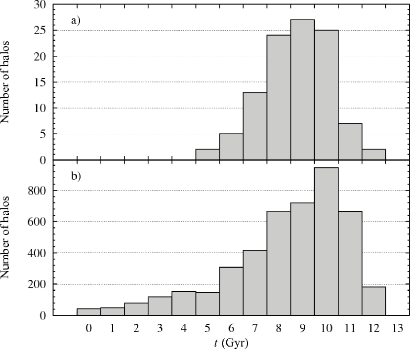
Figure 1: The number of halos drawn from the Millenium Simulation with particle numbers a) $175<N_{\mathrm{p}}<185$ and b) $35<N_{\mathrm{p}}<45$ at $z=0$, binned as a function of how many gigayears ago these halos first reached particles number above a) 100 and b) 20. Halos that undergo a major merger after their formation are explicitly excluded from this tally.

It is clear from Fig. 1 that the peak of halo formation is situated at about 10 Gyr ago, with the majority of halos having formed between 8 and 11 Gyr ago. A closer inspection of both panels of Fig. 1 reveals that the formation rate of the least massive halos, presented in panel b), peaks at $\approx 10$ Gyr ago. This is about 1 Gyr earlier than the formation rate of their more massive analogs, presented in panel a). Extrapolating towards the even lower masses of the galaxies we modeled for the present paper, one could expect the halo formation time to shift to even earlier times, with the oldest halos being formed as early as 12 Gyr ago. We will, therefore, assume that the dark-matter halos of the dwarf galaxies we modeled formed at a redshift $z=4.3$ and neglect further growth of the halo. Furthermore we neglect any environmental effects (e.g. ram-pressure stripping) on the chemical and dynamical evolution of the models. These environmental influences are not always negligible (see e.g. Penarrubia et al. (2007)). Thus, the models describe dwarf galaxy formation as the isolated collapse of a gas cloud in the potential well generated by a spherical dark matter halo and the gas itself (see e.g. Gao & Theuns, 2007).

We use the following cosmological parameters: $h=0.71$, $\Omega_{\mathrm{tot}}=1,\Omega_{\mathrm{matter}}=\Omega_{\mathrm{m}}=0.2383,\Omega_{\mathrm{DM}}=0.1967$ (Spergel et al., 2007), where $h$ is the normalised Hubble constant. The mean density of the Universe as a function of redshift $z$ and Hubble constant $H_{0}=100\,h$ is:

$$\rho_{\mathrm{u}} = \frac{3h^{2}100^{2}}{8\pi G}\left[\Omega_{\mathrm{m}}(1+z)^{3}+1-\Omega_{\mathrm{m}}\right]$$ (18)

$$= 1.99\times 10^{-29}h^{2}\left[\Omega_{\mathrm{m}}(1+z)^{3}+1-\Omega_{\mathrm{m}}\right]\,\mathrm{g}\,\mathrm{cm}^{-3}.$$

We take the over-density of matter to $\rho_{\mathrm{u}}$ to be 5.55, the value when the local flow detaches itself from the Hubble flow, according to the Tolman model of a spherical over-density. $z$ at the start of the simulations is taken to be 4.3, corresponding to approximately 1.5 Gyr after the birth of the universe. The simulation length is set to 10 Gyr, which is long enough to cover the most important part of the star forming period of the simulated galaxies. The density of matter at the start of the simulations is then:

$$\rho_{\mathrm{m}}=5.55\times\rho_{u}.$$ (19)

When the total mass and its density are known we can fix the outer radius:

$$R_{5.55}(z) = \left(\frac{3}{4\pi}\right)^{1/3}\left(\frac{M_{\mathrm{T}}}{\rho_{\mathrm{m}}}\right)^{1/3}$$ (20)

$$= \frac{0.09617}{5.55^{1/3}}\left[\frac{M_{\mathrm{T}}}{h^{2}\left(\Omega_{\mathrm{m}}(1+z)^{3}+1-\Omega_{\mathrm{m}}\right)}\right]^{1/3},$$

where $M_{\mathrm{T}}$ is expressed in $\mathrm{M}_{\sun}$ and $R_{5.55}$ in kpc. At the start of the simulations the gas particles are randomly distributed in a sphere with radius given by equation (20). The gas particles are initially at rest, their initial metallicity is set to $10^{-4}\ Z_{\sun}$ and their initial temperature is $10^{4}$ K.

Several choices are possible for a DM profile. There is the NFW profile, deduced from simulations in Navarro et al. (1997). However observations as well as simulations seem to imply that the DM halo has a central core rather than a cusp (Salucci & Persic, 1997; Merritt et al., 2006; Gentile et al., 2007, and references therein). Other previously used profiles include the modified isothermal sphere (Binney & Tremaine, 1987) or the King profile (e.g. Mori et al., 1999), see Binney & Tremaine (1987). For the DM halo we choose the Kuz’min Kutuzov (KK) profile as presented by Dejonghe & de Zeeuw (1988). The KK profile has several distinct advantages : it is, apart from a numerically well-behaved integral, analytical, and it has a central core. Furthermore, Sellwood & Valluri (1997) have carried out a stability analysis of the KK halo, concluding that haloes with flattening up to E7 are stable. The density of this model is given by:

$$\rho_{\mathrm{KK}}(R,z) = \frac{Mc^{2}}{4\pi}\frac{(a^{2}+c^{2})R^{2}+2a^{2}z^{2}+}{(a^{2}c^{2}+c^{2}R^{2}+a^{2}z^{2})^{3/2}}$$ (21)

$$\frac{2a^{2}c^{2}+a^{4}+3a^{2}\sqrt{a^{2}c^{2}+c^{2}R^{2}+a^{2}z^{2}}}{(R^{2}+z^{2}+a^{2}+2\sqrt{a^{2}c^{2}+c^{2}R^{2}+a^{2}z^{2}})^{3/2}},$$

with $a$ and $c$ parameters controlling the length of the semi-major and semi-minor axis respectively, $R$ is the distance in the $xy$–plane and $z$ is the distance normal to this plane.

We generated the DM halo using a standard Monte Carlo sampling technique. For each particle we first generate three coordinates $R,\phi,z$, distributed as $\rho_{\mathrm{KK}}$ (equation (21)). Then $v_{\mathrm{R}},v_{\mathrm{\phi}}$ and $v_{\mathrm{z}}$ are found using a standard acceptance-rejectance technique using the distribution function of the KK model. The halo density is set to zero outside the equipotential surface $\Psi_{\mathrm{KK}}(R,z)=\Psi_{\mathrm{KK}}(R_{\mathrm{cut}},0)$, with $R_{\mathrm{cut}}=25$ (units $(a+c)$). This large value ensures that the effect of this cut-off on the halo’s stability is negligible. We explicitly checked the halo’s stability by letting it evolve in isolation for the same duration as the science simulations.

Now that we have fixed the cosmological parameters (including the ratio of DM mass to gas mass), we are left with 3 parameters determining the model: $M_{\mathrm{tot}},a$ and $c$. $c$ determines the amount of flattening we want for the halo, where $a=c$ gives a spherical halo. As we restrict ourselves here to spherical systems we set $c=a$. To eliminate a further parameter we set, analogous to $R_{5.55}$ in equation (20),

$$a=C\sqrt[3]{M_{\mathrm{tot}}}\ \frac{\textrm{kpc}}{\sqrt[3]{M_{\sun}}},$$ (22)

where $C$ is fixed by associating one value of $a$ with a value of $M_{\mathrm{tot}}$. Several values of $C$ are explored with our models. This leaves us with one parameter to vary in a series of simulations: $M_{\mathrm{tot}}$.

4 Results

In the following sections we discuss the models. Information about these models can be found in Tables 1 (A models) and 3 (C and D models). The A models all have an identical setup, apart from the number of gas particles. The number of DM particles is set to $15\,000$. We use these A models to determine the minimum number of gas particles that is required for the simulations to be numerically converged. The C models represent the “real” models. We compare in detail some structural parameters of the simulated C-model galaxies with those of observed dwarf galaxies, in order to assess how well the simulations reproduce reality. The B models are essentially a larger version of the C models, being identical in setup, apart from a smaller value of $C$ (equation (22): $C=0.000928$. We also sampled the mass range differently: the total mass of the Bx model does not necessarily correspond to the mass of the Cx model (B models: 0.25, 0.3, 0.65, 1, 3, 6 $\times 10^{9}\ M_{\sun}$). This however has no influence on a comparison of the B and C models. The B models are included only to illustrate the effect of varying $C$ on the half-light radius and the central velocity dispersion of the model galaxies (sections 4.4 and 4.6). They were constructed using $15\,000$ dark matter particles. The two D models do not obey equation (22). They were constructed using an arbitrary (high) value of $C$. The D models are included to show that it is difficult to extend our C models beyond the mass where they break down by fiddling with some parameters.

4.1 Number of particles

To be able to compare simulations covering a wide range of initial masses, the simulations have to converge numerically. At a certain point a further increase of the number of particles should make no (or very little) difference. For this reason we took special care in selecting the SFC (equations 2–4). Results of a first set of simulations for a range of particle numbers (A models) are shown given in Figs. 2–3. These models all use the parameters of the C05 model (see table 3).

Table 1: Information concerning the simulations with varying particle numbers. See text for more details.

Name	$N_{\mathrm{gas}}$	Comments
30k	$3.0\times 10^{4}$	Identical initial conditions files (ICfs).
30k(rd)	$3.0\times 10^{4}$	Resampled ICfs (different Poisson noise).
50k	$5.0\times 10^{4}$	Identical initial conditions files.
75k	$7.5\times 10^{4}$	Identical initial conditions files.
100k	$10.0\times 10^{4}$	Identical initial conditions files.

We use the models listed in table 1 to investigate the dependence of the models on the gas-particle number. These models are all different realisations of the same set-up: that of the C05 model (see table 3). The 30k(rd), 50k and 75k sets consist of 5 simulations; the 30k set of 6 simulations and the 100k set of 3 simulations. The simulations of the 30k set all start from the same initial conditions file, only the random number seed of the stochastic star formation recipy (eq. (7)) varies between simulations. The same goes for the 50k, 75k and 100k sets of simulations. For the 30k(rd) set, the initial conditions file was resampled for each simulation, i.e. they have variable Poisson noise at constant gas-particle number. The number of dark matter particles was kept constant at $30\,000$ particles for all simulations.

A first indication of the global behaviour of the models is shown in Fig. 2 where we plotted the mean SFRs of the sets of models listed in 1, with $1\sigma$ “errorbars” quantifying the variation between the simulations belonging to each set. As a reference, the SFR of the C05 model is also plotted. Obviously, the global SFRs are qualitatively and quantitatively in good agreement and they do not change significantly with gas-particle number. Of course, slight differences between the different sets of models during the first star-formation peaks are amplified towards the later peaks.

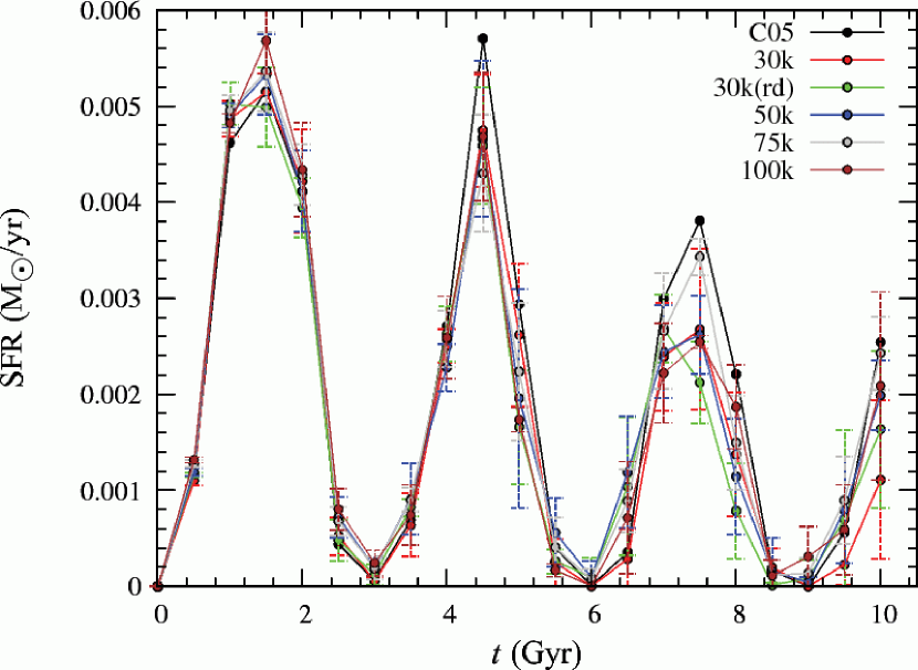
Figure 2: Star Formation Rate (SFR, in M_☉ yr^-1) as a function of time (Gyr) for simulations with varying particle numbers. See text and table 1 for more details.

In figure 3 we plot different observables as a function of stellar mass for the models listed in table 1 as well as the C05 model. We also plot a line connecting the C-series models. Apparently, simulations with higher numbers of gas particles tend to form slightly more stars, the difference between the 30k and 75k sets of simulations being of the order of 10% in terms of stellar mass and with comparable differences on the other observables. There is however no straightforward converging behaviour as the 100k set forms on average less stars than the 75k set. The least well constrained quantity is the percentage of retained gas, with a 30% increase between the 30k and 75k models. Clearly, the scatter between the individual models diminishes towards larger gas-particle numbers but increasing the gas particle number beyond $75\,000$ seems to have no further effect. We conclude that if one wants to compare an individual model in detail to an observed galaxy, it seems advisable to use at least $100\,000$ gas particles in order to minimize the model-to-model scactter. For a comparison between observed and model photometric and kinematic scaling relations, a gas-particle number of $30\,000$ should suffice. The model-to-model scatter is sufficiently small and, in any case, this scatter moves models along the scaling relations so the latter will not be significantly affected. This conclusion is a lot stricter than the one reached in Lia et al. (2000), where the requirement of comparable star formation histories resulted in $N_{\mathrm{gas}}\geq 10\,000$.

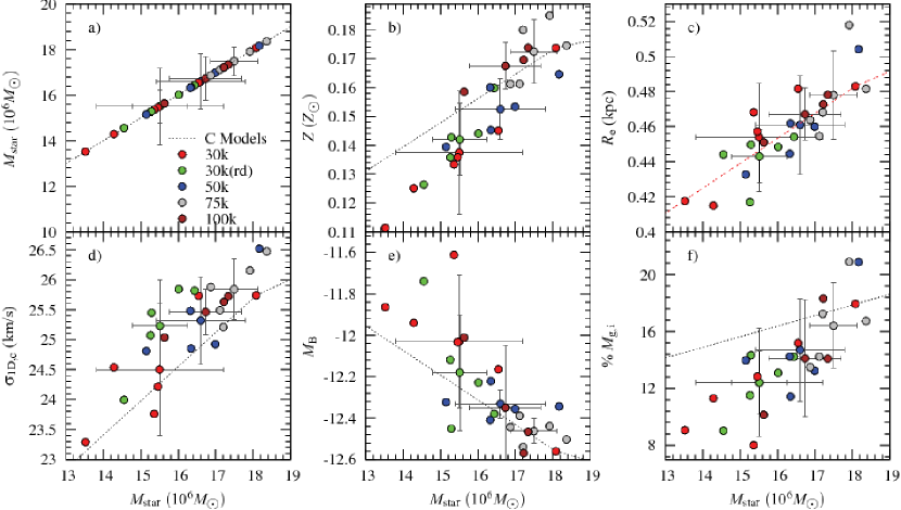
Figure 3: Variation of model observables as a function of gas particle number, shown for the models listed in table 1. The dash-dotted line connects the points of the C models. The symbol at the center of the error-bars indicates to which models these bars belong (it is not a datapoint).

To assess the number of dark matter particles to be used in the simulations, we constructed a further series of models (see table 2). For the 15kdm we started from the same initial conditions file and used 5 different random number seeds for the star formation recipy. The same was done for the 30kdm models. For the 5k-to-25k and 30k-to-60k models the number of dark matter particles was varied whilst retaining the initial conditions for the gas particles. Only 1 run per initial conditions file was done for these models. Results are shown in Fig. 4. Two important conclusions can be drawn from this figure: (i) there is no significant decrease of the scatter on the individual models as a result of an increase in dark matter particles and (ii) DM particle numbers of $15\,000$ and up seem to be sufficient to capture enough physics to closely follow the model relations. Indeed, apart from the leftmost two blue points in each plot (which correspond to $5\,000$ and $10\,000$ DM particles) all the models follow the C model relations. Although we do not rule out a decrease of the scatter on individual models as the number of dark matter particles is further increased, the above two results allow us to use $30\,000$ dark matter particles to investigate the relations our model galaxies follow.

Moreover, we performed a series of simulations with C09 initial conditions but with the number of gas particles increased from $30\,000$ to $40\,000$, $50\,000$, and $60\,000$. Due to star formation, the 60k run reached a total of $200\,000$ particles after 5 Gyr and became impracticably slow and we decided to stop it. Comparing these models, we found that no observable scales directly with the number of gas particles and that the model-to-model scatter on the observables is too small to affect our results and conclusions.

Table 2: Information concerning the simulations with varying dark matter particle numbers. ($N_{\mathrm{gas}}=30\,000$)

Name	$N_{\mathrm{DM}}$	# runs
15kdm	$1.5\times 10^{4}$	5
30kdm	$3.0\times 10^{4}$	5
5k-to-25k	$(0.5,1,1.5,2,2.5)\times 10^{4}$
30k-to-60k	$(3,3.5,4,4.5,5,6)\times 10^{4}$

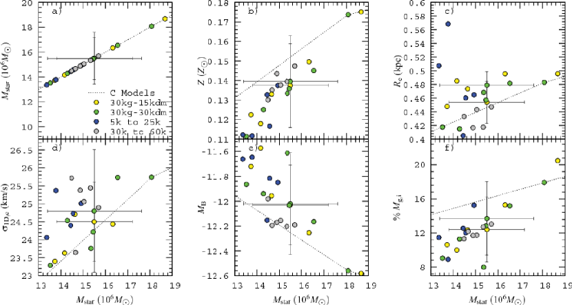
Figure 4: Variation of model observables as a function of the dark matter particle number. The dash-dotted line connects the points of the C models. The symbol at the center of the error-bars indicates to which models these bars belong (it is not a datapoint). The leftmost two blue points in each figure are the models with $5\,000$ and $10\,000$ DM particles (from left to right). For clarity: the larger of the two sets of error-bars in each figure belong to the 30kg-30kdm models. See table 2 for more information about the models.

In conclusion: for our production run models (C and D models) we use $30\,000$ gas particles and $30\,000$ dark matter particles. These numbers used in are an improvement over Chiosi & Carraro (2002), who use $10\,000$ particles for dark and baryonic matter. They are less than the $100\,000$ particles for DM and BM used by Stinson et al. (2007), but we have nevertheless demonstrated that this resolution is sufficient to capture the essentials of the physics.

4.2 Surface brightness Profile

Table 3: Summary of various physical quantities for models C and D (at $t=10$ Gyr). (1) Model name (2) Initial gas mass ($10^{6}\ M_{\sun}$) (3) Initial dark matter mass ($10^{6}\ M_{\sun}$) (4) $a$ for the DM halo (kpc)(see eq. (21)) (5) Absolute magnitude in the blue band (6) Absolute magnitude in the visual band (7) $B-R$ (8) Total final star mass ($10^{6}\ M_{\sun}$) (9) Percentage of initial gas mass remaining ($<$ 30 kpc) (10) Percentage of gas blown out ($>$ 30 kpc) (11) Half-light radius (kpc) (12) One dimensional central velocity dispersion (km s-1) (13) Metallicity ($Z_{\sun}=0.02$)

Run	$M_{\mathrm{g,i}}$	$M_{\mathrm{DM,i}}$	$a$	$M_{\mathrm{B}}$	$M_{\mathrm{V}}$	$B-R$	$M_{\mathrm{star}}$	% $M_{\mathrm{g,i}}$	% BO	$R_{\mathrm{e}}$	$\sigma_{\mathrm{1D,c}}$	$Z(Z_{\sun})$
C01	44	206	0.439	-8.12	-8.72	1.067	0.44	21.0	78.0	0.16	9.6	0.048
C02	52	248	0.466	-8.97	-9.51	0.981	0.81	19.5	78.9	0.18	11.5	0.052
C03	70	330	0.513	-9.89	-10.44	0.997	2.0	15.6	81.6	0.23	14.0	0.045
C04	105	495	0.587	-11.14	-11.68	0.973	6.2	9.1	85.0	0.31	18.9	0.073
C05	140	660	0.646	-12.56	-13.03	0.878	18	17.9	69.1	0.48	25.7	0.174
C06	175	825	0.696	-13.58	-14.02	0.831	38	32.7	45.7	0.67	31.5	0.230
C07	262	1238	0.797	-14.20	-14.83	1.105	122	36.6	16.5	0.76	39.3	0.379
C08	349	1651	0.877	-14.97	-15.56	1.043	228	22.7	11.5	0.62	43.0	0.535
C09	524	2476	1.004	-15.11	-15.77	1.162	393	17.4	6.80	0.57	46.7	0.620
D01	873	4127	4.000	-16.04	-16.61	1.023	579	29.0	4.2	1.13	35.2	0.470
D02	873	4127	6.000	-16.37	-16.82	0.843	488	39.4	4.4	1.26	30.9	0.373

The surface brightness (SB) profile of elliptical galaxies is described well by the de Vaucouleurs $R^{1/4}$ law, whereas dwarf elliptical galaxies are fitted better by an exponential law (see e.g. Jerjen & Binggeli, 1997; Graham & Guzmán, 2003, and references therein). Both profiles are encompassed by Sérsics $R^{1/n}$ law:

$$I(R)=I_{0}\exp{\left\{-\left(\frac{R}{R_{0}}\right)^{\left(1/n\right)}\right\}}.$$ (23)

In Fig. 5 we present a plot of the surface brightness profiles of the C model galaxies as well as their respective best fitting Sérsic profiles. In Fig. 6 we compare the Sérsic parameters $n$ and $\mu_{\mathrm{0}}$ (or $I_{\mathrm{0}}$) for the models with data taken from Graham & Guzmán (2003), De Rijcke et al. (2008) and Mieske et al. (2007). As seen in Fig. 5, the correspondence with a Sérsic profile is excellent. The more massive models ($M_{\mathrm{B}}<-13$ mag) also have SB profiles that closely follow the Sérsic law. Comparison with data in Fig. 6 for the C models shows that $n$ as well as $\mu_{\mathrm{0}}$ are in good correspondence with observations. A variant of the third Sérsic parameter $R_{\mathrm{0}}$, the half-light radius $R_{\mathrm{e}}$, is discussed in section 4.4. The D models perform worse than the C models : whilst $\mu_{\mathrm{0}}$ is only somewhat too low, the values for $n$ are too low. This indicates that the SF should be more centrally concentrated. This is easily understood when considering Table 3: by construction the D models have a large radius, naturally decreasing the resulting $\mu_{\mathrm{0}}$ and $n$.

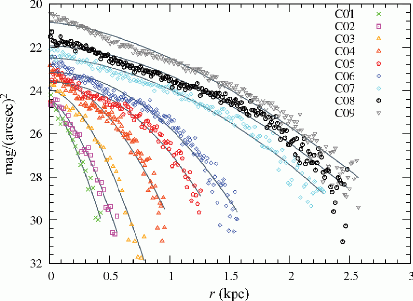
Figure 5: Surface brightness (SB, in mag arcsec^-2) as a function of radius (kpc) for simulations with varying initial mass. The full lines are the best fitting Sérsic profiles.

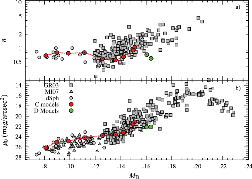
Figure 6: Upper panel: Sérsic index $n$ as a function of blue broad band magnitude $M_{\mathrm{B}}$. Lower panel: central surface brightness $\mu_{\mathrm{0}}$ (mag arcsec^-2) from the Sérsic fit to the models as a function of $M_{\mathrm{B}}$. Data taken from Graham & Guzmán (2003), De Rijcke et al. (2008) and (lower panel only) Mieske et al. (2007) (the canonical value of 0.7 was added to absolute magnitudes and surface brightnesses in the $V$ band to mimic their respective counterparts in the $B$ band).

4.3 Star Formation Rate

The SFR of galaxies is an important tool for the study of their evolution. Observations indicate that the Star Formation Histories of dwarf galaxies are varied and have a burst-like nature (e.g. Smecker-Hane et al., 1996; Mateo, 1998, and references therein). This phenomenon was successfully reproduced by N–body simulations (Chiosi & Carraro, 2002; Stinson et al., 2007). Dellenbusch et al. (2007) find ongoing star formation in their sample of observed dwarf galaxies. They also note and an absence of any indication of a recent major interaction. These observations can be readily explained by invoking the burst-like nature of star formation in dwarf galaxies.

In Fig. 7 we plot the SFRs of the C models.

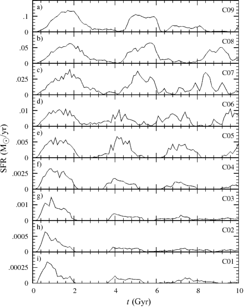
Figure 7: SFR (M_☉ yr-1) as a function of time (Gyr) for the C models.

We immediately see that the SFR is of a burst-like nature. As there is 10 to 30 per cent of the initial gas mass left at the end of the simulations (Table 3) there is still fuel for further star formation. Most dwarf elliptical (dE) galaxies are found to be almost devoid of gas (Young & Lo, 1997; Mateo, 1998; Conselice et al., 2003; De Rijcke et al., 2003; Bouchard et al., 2005; Buyle et al., 2005). There is however a very strong morphological segregation of dwarf elliptical galaxies (Binggeli et al., 1990). These authors found that almost all dEs are found in clusters or in dense groups, or as companions (satellites) of a massive galaxy. This implies that dwarf elliptical galaxies, found in dense environments, are subject to significant ram-pressure stripping which depletes their gas reservoirs (Mori & Burkert, 2000; Marcolini et al., 2003). This physical process is not included in our simulations so the modelled galaxies retain part of their gas reservoir.

In Fig. 8 we plot the temperature distribution of the gas particles as a function of their density, for the C05 model, at 4 different times: 1, 2.6 , 7 and 8.5 Gyr. In each figure the lower right quadrant contains the gas particles that satisfy the density and temperature criterion for star formation (eqs. (3) and (4)). From Fig. 7 we can see that at 1 and 7 Gyr the galaxy is undergoing a star-burst. At 2.6 and 8.5 Gyr there is no star-formation. From Fig. 8 it is clear that the quiescent intervals between star-bursts are caused by a decrease in gas density. This in turn is a result of the stellar feedback: the entire central population of gas particles is pushed to lower densities, inhibiting further star formation. On the lower left part of each figure we can see gas particles being blown out of the galaxy, resulting in a declining density and temperature. On panels b), c) and d) we can clearly see the outward propagation of the gas particles expelled by the different starbursts towards the lower left corner of the figure.

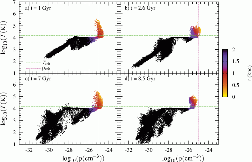
Figure 8: The logarithm of the temperature, $T$, versus the density, $\rho$, for the gas particles, at 4 different times (C05 model). Particles are colour-coded according to their distance from the galaxy centre $r$.

The cause of the burst-like behaviour can be seen on Fig. 9, where the effects of the various SFC are plotted for model C06. From the upper panel we learn that the temperature criterion (eq. 2) has little influence on SF, prohibiting a small fraction of the gas particles from forming stars. The divergence criterion (eq. 3) is more restrictive, allowing on average 30 per cent of the gas particles to form stars and restricting the star formation to the more central regions of the galaxy. The real control over star formation resides however in the density criterion (eq. 4). Not only is this criterion very restrictive (which of course depends on the value of $\rho_{c}$), typically allowing 5–10 per cent of the gas particles to form stars, it is also responsible for the burst-like behaviour the star formation. Star formation is in a sense a self-regulating process: high density gives high SF, resulting in a lot of SNe which will heat up and disperse the gas, leading to the end of the SF episode. As the temperature criterion has only little effect it could be dropped altogether (no unrealistic star formation should take place in hot regions because hot clouds with high density will cool fast anyway, hot clouds with low density are not allowed to form stars). Kravtsov (2003); Li et al. (2005, 2006) use only the density criterion in their N–body/SPH simulations, while using enough particles to satisfy the Jeans resolution criterion (Bate & Burkert, 1997) and thus resolving Jeans instability in molecular clouds. They find that the Schmidt law (eq. 5) is a result of gravitational instability and thus of the overall density distribution, which validates our SF because we also find it to be –mainly– determined by the density distribution.

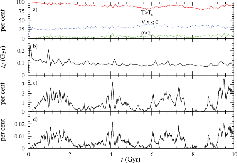
Figure 9: Data taken from the C06 model. a) Percentage of gas particles satisfying a SF criterion. b): Average dynamical time (Gyr) for gas particles within 0.5 kpc of the galaxy centre. c) Percentage of gas particles satisfying the 3 SFC. d) Percentage of gas particles forming stars.

When comparing panels a) and b) of Fig. 9 we see the behaviour expected from $t_{d}$ (equation (6)): peaks when there are few particles with high density and vice verse, with an approximately constant value otherwise ($\approx 0.12$ Gyr). When going from panel 3) to panel 4), equation (7) is applied. Because of the moderate variations of $t_{d}$ there is little qualitative difference between the two panels, although the quantitative difference is large (factor 100). The use of equation (7) is thus twofold: on the one hand it serves as a means to drastically reduce the number of star forming gas particles, on the other hand it introduces an independence of the number of time-steps into the star formation prescription.

In Fig. 10 we show a measure of the distribution of SF in space for our models. The apparent rise of the SFR towards larger radii (within a starburst) is caused by the rise in volume of the spherical bins. The volume-averaged SFR, plotted in Fig. 11, shows that there is actually more SF in the centre of the Model galaxies. We can also see that in our more massive models, during the first starburst, SF takes an increasing amount of time to reach the outskirts of the galaxy. On panels a), c) and d) of Fig. 10 we see that star formation becomes more centrally concentrated as time passes: each subsequent star-burst is confined to a smaller radius. For model C02 (panel d)) this effect is even stronger: the first star-burst contains two phases, with SF in the first phase extending to about $\approx$ 0.5 kpc, in the second phase to $\approx$ 0.3 kpc. Our models thus naturally reproduce the observations of Tolstoy et al. (2004). These authors found two distinct ancient components in the Sculptor dSPH, the metal-poor component being more extended in space. They considered the interplay of gas infall due to gravitation and supernova feedback to be a possible explanation. Battaglia et al. (2006) found a similar effect in the Fornax dSph: they found 3 distinct stellar populations (ages $>10$ Gyr, 2–8 Gyr and $<100$ Myr), where the younger, more metal-rich populations are found to occupy a smaller region of space. We can immediately qualitatively compare these findings with our C04 Model, which also gives rise to 3 different populations, with each subsequent population being more metal-rich and confined to a smaller region in space. Mashchenko et al. (2007) offer a different explanation: the DM, gravitationally heated because of gas motion, in turn heats the stellar population. As the older (metal poor) population has somewhat more time to be heated than the metal rich population, it will occupy a larger region in space. These authors, however, do not provide quantitative predictions based on this scenario. Note that the apparent absence of SF in the inner radial bin, visible in Fig 11, is an artifact caused by small number statistics as the size of the volume over which we calculate the star-formation density becomes small compared with the inter-particle distances.

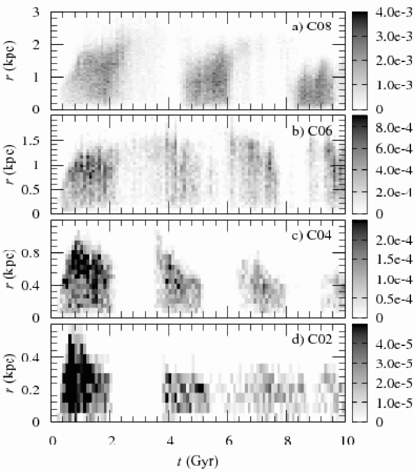
Figure 10: SFR ($M_{\sun}$/Gyr) as a function of time and distance from the galaxy centre, for four different models. The SFR is integrated over spherical shells with width $r_{\mathrm{max}}/50$, with $r_{\mathrm{max}}$ from the top to the bottom panel: 3,2,1.2,0.6 kpc respectively.

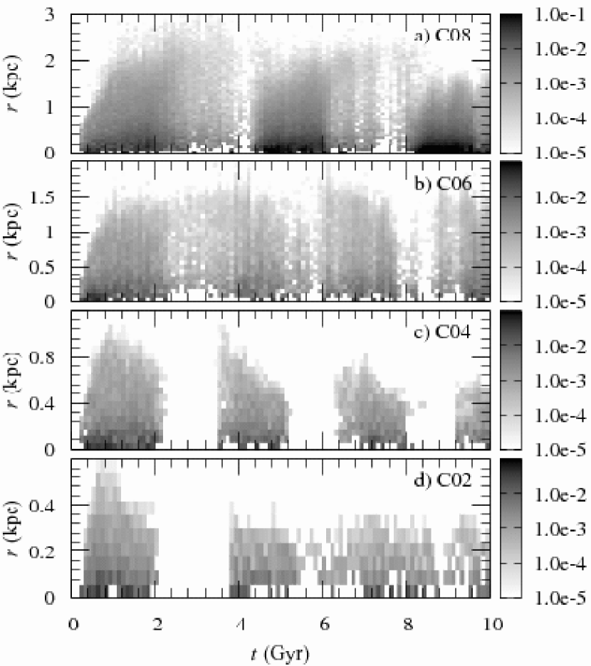
Figure 11: SF density ($M_{\sun}$/Gyr/kpc³) as a function of time and distance from the galaxy centre, for four different models. The spherical bins are equal to those of Fig. 10.

From Table 3 we can conclude that blow-out of gas in the models is not very efficient. Although the least massive models easily lose up to 80 per cent of their gas, this declines to around 5 per cent for the most massive C models and for the D models. This difference in dynamical evolution is shown in Fig. 12, showing the evolution of the gaseous component of 2 models, as a function of time. While the C06 model is able to retain most of the gas and steadily converts it into stars, the C02 model is clearly not massive enough to be able to capture a large amount of gas. Mac Low & Ferrara (1999) find that blow-away occurs for $M_{\mathrm{gas}}$ up to $10^{5}-10^{6}\ M_{\sun}$, and that no blow-out of gas occurs for gas masses $\approx 10^{8}-10^{10}\ M_{\sun}$ (depending on the energy released by SNe). These observations are broadly consistent with our results: gas loss is very small for initial gas masses $\geq 4\times 10^{8}\ M_{\sun}$. Our upper limit for blow-away is $\approx 4\times 10^{7}M_{\sun}$ (C01 model). Ferrara & Tolstoy (2000) find a comparable limit for blow-out as Mac Low & Ferrara (1999): $M_{\mathrm{gas}}\approx 10^{8}-10^{9}\ M_{\sun}$, also in good agreement with our results.

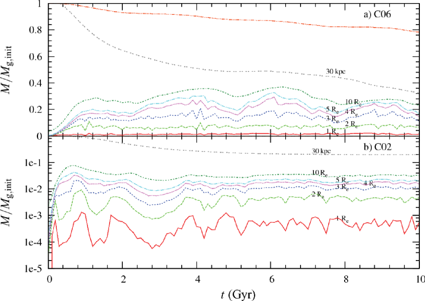
Figure 12: Evolution of the gas mass as a function of time (Gyr), for Models C06 (upper panel) and C02 (lower panel). The different lines show the fraction (mass divided by the initial gas mass) of the gas mass that is contained in a sphere with a given radius ($1R_{\mathrm{e}},2R_{\mathrm{e}},3R_{\mathrm{e}},4R_{\mathrm{e}},5R_{\mathrm{e}},10R_{\mathrm{e}},30\ \mathrm{kpc}$). The top line shows the fractional gas mass remaining (i.e. not converted into stars.) $R_{\mathrm{e}}$ is the half-light radius at the end of the simulation (see Table 3). The top line for panel b) is not visible because it is $\approx 1$.

4.4 Half-light radius

The half-light radius, the radius of a galaxy containing half its total luminosity, is an important diagnostic parameter in simulations of galaxy formation. Large deviations from values dictated by observations hint at an erroneous spatial distribution of the star formation of model galaxies. Instead of using the three dimensional half-mass radius for $R_{\mathrm{e}}$, we chose to calculate the value accessible to observers: the two dimensional half-luminosity radius. We first projected the light distribution of the models onto the $xy$ plane and derived the cumulative luminosity function $L(R)$ as a function of radius. The value of $R$ where $L(R)$ reaches half its maximum is then the half-light radius. Results for the models are shown in Fig. 13, where the logarithm of $R_{\mathrm{e}}$ is shown as a function of $M_{\mathrm{B}}$. Throughout the simulations we found that the half-light radius of a model galaxy is very sensitive to the setup (e.g. initial conditions) of the simulations. Restraining it to a reasonable value is a far from trivial task, as can also be seen by the large variations in the values of the CC02 models (Fig. 13). Comparison of the data-points for the B and C models show that increasing the size of the DM halo results in an increase of the galaxy half-light radius. When the models are to be compared to the CC02 models it should be to the CC02-B models, because those have initial densities closely resembling ours (the over-density of matter in the CC02-B models is set to 1: $\rho_{\mathrm{gas}}=M_{\mathrm{gas}}/M_{\mathrm{DM}}\times\rho_{\mathrm{u}}\approx 0.11\,\rho_{\mathrm{u}}$, whereas the CC02-A models have $\rho_{\mathrm{gas}}\approx 22\,\rho_{\mathrm{u}}$. We have $\rho_{\mathrm{gas}}=M_{\mathrm{gas}}/M_{\mathrm{DM}}\times 5.55\times 0.3\,\rho_{\mathrm{u}}\approx 0.35\,\rho_{\mathrm{u}}$ (see eq. (19))). Although somewhat too large, the model galaxies (B and C) perform reasonably well in the range $M_{\mathrm{B}}\in[-6,-15]$ mag. When we look at the larger models ($M_{\mathrm{B}}<-15$ mag) we see that $R_{\mathrm{e}}$ decreases with increasing mass, signalling a much too central concentration of star formation compared with observations. A plausible explanation for this failure is that the breakdown of the models signals where the effects of hierarchical merging can no longer be neglected in the formation of galaxies, and thus that the simple initial conditions are no longer accurate in this region. When looking at the D models, where we chose $a$ for the DM haloes to be an arbitrary larger value (Table 3), we see that it is possible to produce massive dwarf galaxies that do comply with observations, using a more extended halo than dictated by equation (22). Here the correspondence with observations is excellent, showing not only that we can indeed regard the extent of the halo (within our set framework of star formation, feedback, …) as the decisive factor concerning $R_{\mathrm{e}}$ but also that we could fine-tune it, without changing any other parameters, to get excellent agreement between theory and observations over the entire dwarf magnitude range $M_{\mathrm{B}}\in[-8,-18]$ mag for $R_{\mathrm{e}}$. As the discussion in section 4.2 shows, however, these models deviate from the expected Sérsic profile. This deviation could be alleviated by changing (reducing) $a$. We feel however that fiddling with parameters from model to model to be able to cover the entire magnitude range of the dwarf galaxies with excellent precision would not give much insight in the physics involved. A preferred strategy would be to study the evolution of dwarf galaxies in a fully cosmological setting, or to derive information about the initial conditions (extent and shape of the DM haloes, the ratio of gas mass to DM mass, …) directly from numerical simulations. This is beyond the scope of this paper. We limit ourselves in this paper to the mass range where our chosen set of parameters gives good results. We note that the SAMs of Nagashima et al. (2005) seem to be suffering from the same behaviour of $R_{\mathrm{e}}$, it being rather large for small galaxies. There it is argued that this is a result of either the limited resolution of their N-body simulations, used to construct a merger tree, or that the SF timescale at high redshift is too long.

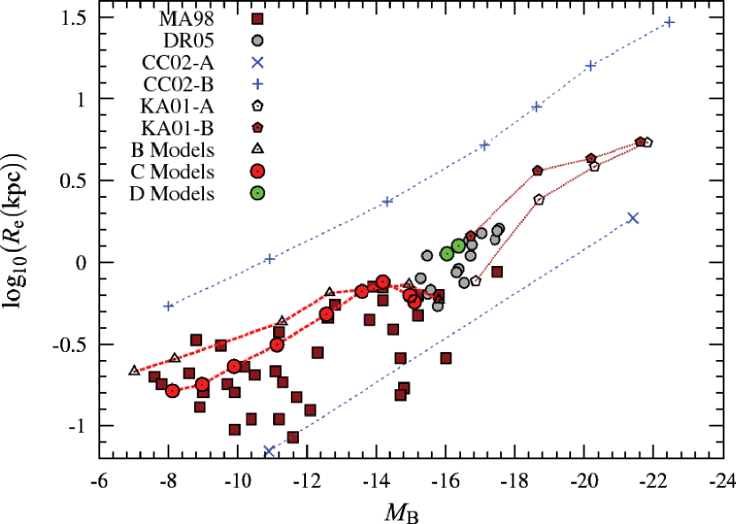
Figure 13: Logarithm of the half-light radius $R_{\mathrm{e}}$ as a function of the absolute magnitude in the B-band $M_{\mathrm{B}}$ for several data-sets (observations: MA98 (Mateo, 1998) (filled boxes: data that only appears in this plot), DR05 (De Rijcke et al., 2005), theory: CC02 (Chiosi & Carraro, 2002), KA01 (Kawata, 2001)) as well as the models.

4.5 Colour

When comparing the $B-V$ colour of the models with observations (Fig. 14) we find good agreement. Besides the value of $B-V$ at $t=10$ Gyr we also plotted the minimum and maximum value in the interval 7.4–10 Gyr for each simulation, as a function of $M_{\mathrm{B}}$ at those times (open tilted squares). This gives an idea of the variation of $B-V$ during the evolution of the model galaxies. This variation is significant, which can be readily understood when looking at e.g. Fig. 7, as star-bursts tend to lower $B-V$ because of the formation of bright blue stars (see the discussion in Chiosi & Carraro, 2002). In this view the higher values for the CC02 models can be explained by looking at their fig. 2: all models have 1 predominant SF peak, no SF takes place after 6 Gyr of evolution, thus excluding the presence of high-luminosity young blue stars. Higher values of $B-V$ could be obtained for the models by e.g. removing the gas content of a model after 1 or 2 SF peaks (as would be expected to happen in a cluster environment). When taking the state of Model C04 at 4 Gyr, which is between the first and second SF peak, and calculating luminosities as if the galaxy has an age of 10 Gyr, thus mimicking quiet evolution after the first SF peak, we get a $B-V$ value of 0.71, close to the CC02 values.

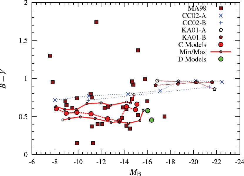
Figure 14: $B-V$ colour of observed galaxies as well as the model galaxies as a function of blue magnitude $M_{\mathrm{B}}$.

4.6 Central velocity dispersion

We used the one dimensional central velocity dispersion, which is the three dimensional velocity dispersion ($\sigma$) divided by $\sqrt{3}$. Although, from an observational point of view, there are better measures for $\sigma$ (e.g. light weighted average $\sigma$) because of possible nucleation of dwarf galaxies, $\sigma_{\mathrm{1D,c}}$ is a good enough measure for our comparison. We measured the central $\sigma$ by fitting an exponential function to the dispersion profile, of which we retain the central value. Results are shown in Fig. 15. Except for the least and the most massive C models, $\sigma$ is too high. The correspondence for the D models is however excellent. Overall we find reasonable convergence between models and observations within a factor of 2 (0.3 dex). We further note that a comparison of Figs. 13 and 15 learns that raising $a$ (going from the C to the B models) results in an increase of the half-light radius as well as a decrease of central $\sigma$. Because of this we cannot increase $a$ for the light models to get a better fit as this would cause $R_{\mathrm{e}}$ to increase. The combination of $R_{\mathrm{e}}$ and the central $\sigma$ thus provide an excellent tool to evaluate the soundness of halo properties within a certain framework of galaxy formation.

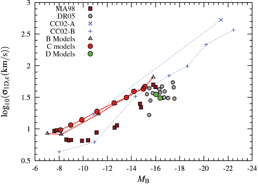
Figure 15: Logarithm of the 1-dimensional central velocity dispersion $\sigma$ (km s-1) as a function of the absolute magnitude in the B-band $M_{\mathrm{B}}$ for several data-sets, as well as the models.

4.7 Metallicity

In Fig. 16 we plot metallicity ($\log_{10}(Z/Z_{\sun})_{\mathrm{B}}$, with $Z_{\sun}=0.02$), for the C and D models as well as 3 sets of data-points. $Z$ for our models is $Z_{\mathrm{B}}$, the light-weighted blue band metallicity. New and improved information concerning the age and metallicity of dwarf galaxies has become available during the recent years (Geha et al., 2003; van Zee et al., 2004; Michielsen et al., 2007; Penny & Conselice, 2007). Dwarf galaxies appear to be young, with $[Z/\mathrm{H}]$ approximately between -0.5 and 0, and a solar $[\alpha/\mathrm{Fe}]$. Three sets of points are plotted for each model, respectively at $t=2.5,5$ and 10 Gyr. For the CC02 models the maximum metallicity is plotted. The overall trend is that metallicity increases with galaxy (star) mass (see e.g. Tremonti et al., 2004). We see from Fig. 16 that the C models reproduce the observed trend well. The values agree reasonably with the data-points, being on average 0.2 dex too high. For the D models the correspondence with the observations is good. At 2.5 and 5 Gyr all the models correspond excellent with the data-points.

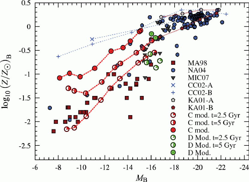
Figure 16: Logarithm of the metallicity of model galaxies (plotted at $t=2.5,5,10$ Gyr) as well as data-points (NA04 (Nagashima & Yoshii, 2004), MIC07 (Michielsen et al., 2007)) as a function of blue magnitude. For the CC02 models the maximum metallicity is plotted.

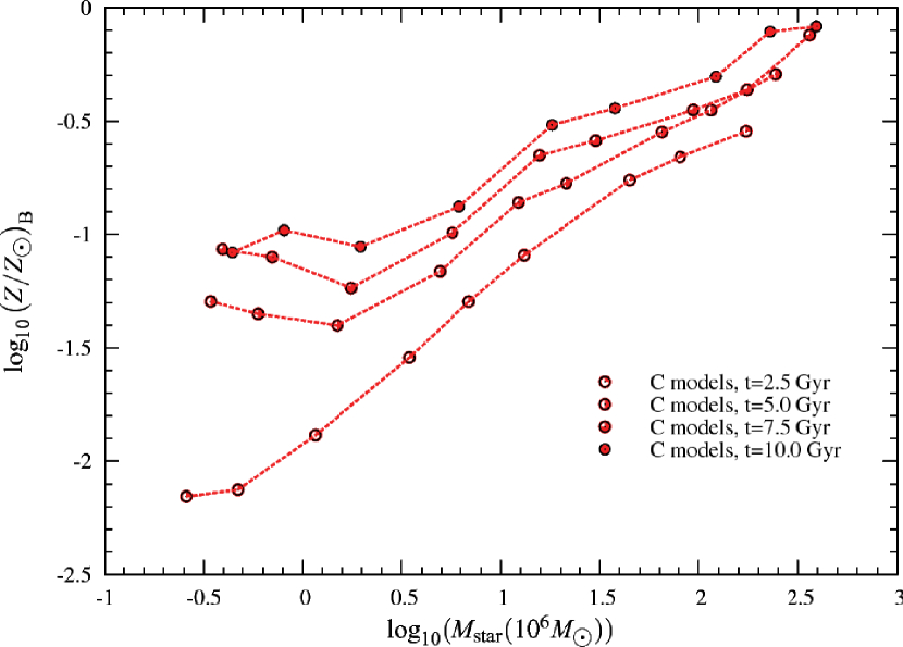
Figure 17: Logarithm of the metallicity $Z_{\mathrm{B}}$ of model galaxies as a function of the logarithm of star mass at 4 different times (from bottom to top: 2.5,5,7.5,10 Gyr) for the C models.

In Fig. 17 we plot $Z$ as a function of stellar mass at 4 different times for the C models. The initial decline of $Z$ with stellar mass is a consequence of the rise of the number of SNe, which is not compensated for by the deepening of the galaxy potential well. This is confirmed by Table 3, where the remaining gas mass is seen to drop when going from model C01 to C03. From the C03 model upwards, the metallicity rises with increasing galaxy mass, indicating that the potential well is steep enough to compensate for the increase in energy input into the ISM. No clear trend concerning the remaining gas of these models can be seen in Table 3.

This effect is not visible in the observational data. It is however unlikely that the decrease of metallicity with stellar mass would be observable in dwarf spheroidal galaxies as it depends strongly on the star formation in the range [3-10] Gyr (fig. 7), and we expect that external processes (e.g. stripping) will greatly affect the evolution of these light systems. Furthermore this effect is model dependent and might be attenuated or even erased when modelling galaxies using a different DM halo.

4.8 The fundamental plane

The fundamental plane (FP) in $\kappa$-space (Bender et al., 1992), as defined by the Virgo galaxies, is given by (Burstein et al., 1997):

$$\kappa_{3}=0.15\,\kappa_{1}+0.43.$$ (24)

where

$$\kappa_{1}= \frac{1}{\sqrt{2}}\log_{10}(R_{\mathrm{e}}\sigma_{\mathrm{c}}^{2}) \kappa_{2}=\frac{1}{\sqrt{6}}\log_{10}(\frac{I_{\mathrm{e}}^{2}\sigma_{\mathrm{c}}^{2}}{R_{\mathrm{e}}~{}})$$

$$\kappa_{3}= \frac{1}{\sqrt{3}}\log_{10}(\frac{\sigma_{\mathrm{c}}^{2}}{I_{\mathrm{e}}R_{\mathrm{e}}})$$ (25)

$I_{\mathrm{e}}$ is the effective surface brightness or the surface brightness within a distance $R_{\mathrm{e}}$ from the galaxy centre. The physical meaning of the $\kappa$ variables can be described as follows: $\kappa_{1}\propto\log_{10}(M),\kappa_{2}\propto\log_{10}(I_{\mathrm{e}}^{3}M/L),\kappa_{3}\propto\log_{10}(M/L)$. Our models are plotted in $\kappa$-space in Fig. 18. We show an edge-on projection of the FP in panel a), a face-on projection in panel b). In Fig. 19 we plot the FP using observed quantities ($R_{\mathrm{e}},\sigma_{\mathrm{c}},I_{\mathrm{e}})$ as coordinates. Fig. 20 shows the deviation of galaxies from the FP. The observational data on panel a) of Fig. 18 learns that the trend of decreasing $M/L$ with decreasing mass is reversed at $\kappa_{1}\approx 2.5$. This indicates that dwarf galaxies and subsequent lighter systems suffer from depletion of baryonic matter relative to dark matter. Our models clearly reproduce this trend. From panel b) we learn that, despite a higher mass-to-light ratio, $\kappa_{2}$ is lower for DGs and light-weight galaxies than for more massive galaxies on the FP. These light-weight galaxies are therefore much fainter and more diffuse than their FP counterparts. Again we clearly reproduce this trend with our models. Figs. 19 and 20 confirm this picture : our models reproduce the deviation of dSphs and dEs from the FP quite well. This deviation can hence be entirely contributed to the shallowness of the galaxy potential well, no stripping effects need to be invoked.

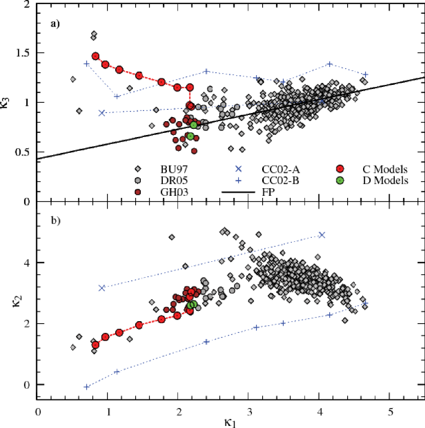
Figure 18: The fundamental plane in $\kappa$-space ($\kappa_{1},\kappa_{2},\kappa_{3}$.). a) edge-on. The solid line is the equation of the FP derived from Virgo galaxies: $\kappa_{3}=0.15\,\kappa_{1}+0.43$ (Burstein et al., 1997, corrected to $H_{0}=70$ km s^-1 Mpc^-1). b) face-on. Data represented by open squares are taken from Burstein et al. (1997), data represented by asterisks are taken from Geha et al. (2003).

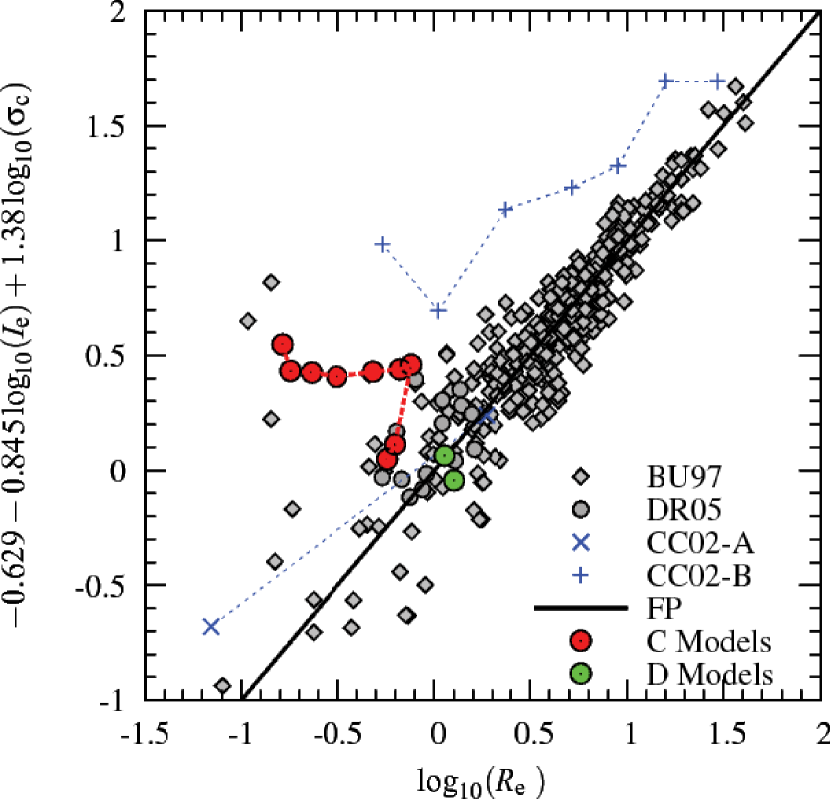
Figure 19: The fundamental plane in physical coordinates: $\log_{10}(R_{\mathrm{e}}~{})=-0.629-0.845\log_{10}(I_{\mathrm{e}})+1.38\log_{10}(\sigma_{\mathrm{c}})$. The full black line shows a side projection of the FP.

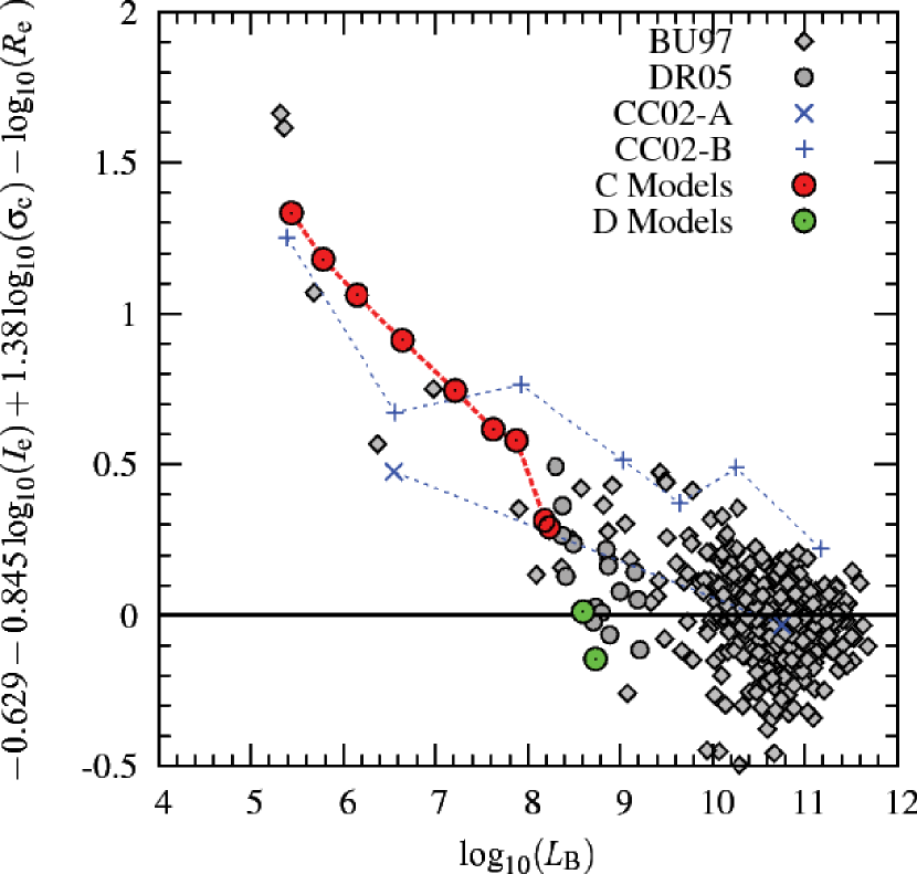
Figure 20: Plot of the deviation from the fundamental plane. The black line represents zero deviation from the FP.

5 Discussion and conclusions

We have presented N–body/SPH models of dwarf galaxies. The basic SPH scheme was modified to include star formation, supernova feedback, chemical enrichment and gas cooling. The simulations start from a homogeneous gas cloud collapsing onto a DM halo. A first series of models (A models) was used to investigate the influence of the gas particle number on the overall evolution of the system. We found that a minimum of 25 000 particles is required to resolve the evolution accurately. Using less particles leads to a reduced first star formation peak. Because of this, the ISM is injected with less energy (less SNe), resulting in higher subsequent SF peaks and hence a larger final stellar mass (Table 1). Based on these experiments, we decided to use 30 000 gas particles and 15 000 DM particles in the simulations.

All our model galaxies exhibit burst-like star formation. This is a direct consequence of star formation in a shallow potential well. Supernovae heat the gas, causing it to expand. The gas density consequently drops below the threshold $\rho_{\mathrm{c}}$ for star formation. After the lapse of an adiabatic cooling period, the gas is again allowed to cool and contract. Star formation thus appears to be a self-regulating mechanism. Since substantial amounts of gas remain in and around the model galaxies throughout the duration of the simulations (see fig. 12), one expects that tidal interactions and ram-pressure stripping in dense environments will have a significant effect on their SFHs.

We compared the model galaxies with observational data in terms of morphology (Sérsic $n$, $R_{\mathrm{e}}$, $\mu_{0}$), kinematics ($\sigma_{\mathrm{1D,0}}$), colour, metallicity and location with respect to the FP ($\kappa_{1},\kappa_{2},\kappa_{3}$). Despite their simplicity, the models do very well in the range $-8>M_{\mathrm{B}}>-15$ mag. The models reproduce the slopes of the size, colour, metallicity, and velocity dispersion vs. luminosity relations very well. The zero-points of these relations are reproduced to within a factor of 2. The position of the model dwarf galaxies in the three-dimensional space spanned by $(R_{\mathrm{e}},\sigma_{\mathrm{1D,0}},I_{\mathrm{e}})$ agrees excellently with the observations. Dwarf galaxies trace a sequence within the FP (i.e. in the $(\kappa_{1},\kappa_{2})$ projection) that is almost orthogonal to that of massive galaxies. In the dwarf regime, the height above the FP (in the $(\kappa_{1},\kappa_{3})$ projection) is a decreasing function of galaxy mass. This is a consequence of less massive galaxies having shallower potentials than more massive ones, decreasing the tendency of the gas to fall into the potential well and increasing the capability of supernovae to support the gas by heating it.

Furthermore we found that a good check for the validity of models is the combination of $R_{\mathrm{e}}$ and $\sigma_{\mathrm{c}}$. $R_{\mathrm{e}}$ is very sensitive to the location of star formation and hence to the time evolution of the density of the ISM. $\sigma_{\mathrm{c}}$ reflects, through the virial theorem, the total amount and distribution of (dark) matter. We demonstrate this using our B and C models, where it can be clearly seen (figs. 13 and 15) that using a more diffuse DM halo indeed raises $R_{\mathrm{e}}$, and at the same time reduces $\sigma_{\mathrm{c}}$.

References

- Bate & Burkert (1997) Bate M. R., Burkert A., 1997, MNRAS, 288, 1060
- Battaglia et al. (2006) Battaglia G., Tolstoy E., Helmi A., Irwin M. J., Letarte B., Jablonka P., Hill V., Venn K. A., Shetrone M. D., Arimoto N., Primas F., Kaufer A., Francois P., Szeifert T., Abel T., Sadakane K., 2006, A&A, 459, 423
- Bender et al. (1992) Bender R., Burstein D., Faber S. M., 1992, ApJ, 399, 462
- Binggeli et al. (1990) Binggeli B., Tarenghi M., Sandage A., 1990, A&A, 228, 42
- Binney & Tremaine (1987) Binney J., Tremaine S., 1987, Galactic dynamics. Princeton, NJ, Princeton University Press, 1987, 747 p.
- Bouchard et al. (2005) Bouchard A., Jerjen H., Da Costa G. S., Ott J., 2005, AJ, 130, 2058
- Buonomo et al. (2000) Buonomo F., Carraro G., Chiosi C., Lia C., 2000, MNRAS, 312, 371
- Burkert & Ruiz-Lapuente (1997) Burkert A., Ruiz-Lapuente P., 1997, ApJ, 480, 297
- Burstein et al. (1997) Burstein D., Bender R., Faber S., Nolthenius R., 1997, AJ, 114, 1365
- Buyle et al. (2005) Buyle P., De Rijcke S., Michielsen D., Baes M., Dejonghe H., 2005, MNRAS, 360, 853
- Chiosi & Carraro (2002) Chiosi C., Carraro G., 2002, MNRAS, 335, 335
- Conselice et al. (2003) Conselice C. J., O’Neil K., Gallagher J. S., Wyse R. F. G., 2003, ApJ, 591, 167
- Couchman et al. (1995) Couchman H. M. P., Thomas P. A., Pearce F. R., 1995, ApJ, 452, 797
- David et al. (1990) David L. P., Forman W., Jones C., 1990, ApJ, 359, 29
- De Rijcke et al. (2005) De Rijcke S., Michielsen D., Dejonghe H., Zeilinger W. W., Hau G. K. T., 2005, A&A, 438, 491
- De Rijcke et al. (2008) De Rijcke S., Penny S. J., Valcke S., Conselice C. J., 2008, in preparation
- De Rijcke et al. (2003) De Rijcke S., Zeilinger W. W., Dejonghe H., Hau G. K. T., 2003, MNRAS, 339, 225
- Dejonghe & de Zeeuw (1988) Dejonghe H., de Zeeuw T., 1988, ApJ, 333, 90
- Dekel & Silk (1986) Dekel A., Silk J., 1986, ApJ, 303, 39
- Dellenbusch et al. (2007) Dellenbusch K. E., Gallagher J. S., Knezek P. M., Noble A. G., 2007, ArXiv e-prints, 710
- Ferguson & Binggeli (1994) Ferguson H. C., Binggeli B., 1994, A&A Rev., 6, 67
- Ferrara & Tolstoy (2000) Ferrara A., Tolstoy E., 2000, MNRAS, 313, 291
- Gao & Theuns (2007) Gao L., Theuns T., 2007, ArXiv e-prints, 709
- Geha et al. (2003) Geha M., Guhathakurta P., van der Marel R. P., 2003, AJ, 126, 1794
- Gentile et al. (2007) Gentile G., Tonini C., Salucci P., 2007, ArXiv Astrophysics e-prints
- Gingold & Monaghan (1977) Gingold R. A., Monaghan J. J., 1977, MNRAS, 181, 375
- Graham & Guzmán (2003) Graham A. W., Guzmán R., 2003, AJ, 125, 2936
- Jerjen & Binggeli (1997) Jerjen H., Binggeli B., 1997, in Arnaboldi M., Da Costa G. S., Saha P., eds, The Nature of Elliptical Galaxies; 2nd Stromlo Symposium Vol. 116 of Astronomical Society of the Pacific Conference Series, Are ”Dwarf” Ellipticals Genuine Ellipticals?. pp 239–+
- Katz (1991) Katz N., 1991, ApJ, 368, 325
- Katz et al. (1996) Katz N., Weinberg D. H., Hernquist L., 1996, ApJS, 105, 19
- Kauffmann et al. (1999) Kauffmann G., Colberg J. M., Diaferio A., White S. D. M., 1999, MNRAS, 303, 188
- Kawata (2001) Kawata D., 2001, ApJ, 558, 598
- Kawata & Gibson (2003) Kawata D., Gibson B. K., 2003, MNRAS, 340, 908
- Kay et al. (2002) Kay S. T., Pearce F. R., Frenk C. S., Jenkins A., 2002, MNRAS, 330, 113
- Kennicutt (1998) Kennicutt Jr. R. C., 1998, ApJ, 498, 541
- Kobayashi (2005) Kobayashi C., 2005, MNRAS, 361, 1216
- Kravtsov (2003) Kravtsov A. V., 2003, ApJl, 590, L1
- Li et al. (2005) Li Y., Mac Low M.-M., Klessen R. S., 2005, ApJl, 620, L19
- Li et al. (2006) Li Y., Mac Low M.-M., Klessen R. S., 2006, ApJ, 639, 879
- Lia et al. (2000) Lia C., Carraro G., Salucci P., 2000, A&A, 360, 76
- Lucy (1977) Lucy L. B., 1977, AJ, 82, 1013
- Mac Low & Ferrara (1999) Mac Low M.-M., Ferrara A., 1999, ApJ, 513, 142
- Marcolini et al. (2003) Marcolini A., Brighenti F., D’Ercole A., 2003, MNRAS, 345, 1329
- Marcolini et al. (2006) Marcolini A., D’Ercole A., Brighenti F., Recchi S., 2006, MNRAS, 371, 643
- Mashchenko et al. (2005) Mashchenko S., Couchman H. M. P., Sills A., 2005, ApJ, 624, 726
- Mashchenko et al. (2007) Mashchenko S., Wadsley J., Couchman H. M. P., 2007, ArXiv e-prints, 711
- Mateo (1998) Mateo M. L., 1998, ARA&A, 36, 435
- Merlin & Chiosi (2006) Merlin E., Chiosi C., 2006, A&A, 457, 437
- Merritt et al. (2006) Merritt D., Graham A. W., Moore B., Diemand J., Terzić B., 2006, AJ, 132, 2685
- Michielsen et al. (2007) Michielsen D., Koleva M., Prugniel P., Zeilinger W. W., De Rijcke S., Dejonghe H., Pasquali A., Ferreras I., Debattista V. P., 2007, ArXiv e-prints, 710
- Mieske et al. (2007) Mieske S., Hilker M., Infante L., Mendes de Oliveira C., 2007, A&A, 463, 503
- Mori & Burkert (2000) Mori M., Burkert A., 2000, ApJ, 538, 559
- Mori et al. (1999) Mori M., Yoshii Y., Nomoto K., 1999, ApJ, 511, 585
- Mori et al. (1997) Mori M., Yoshii Y., Tsujimoto T., Nomoto K., 1997, ApJl, 478, L21+
- Nagashima et al. (2005) Nagashima M., Yahagi H., Enoki M., Yoshii Y., Gouda N., 2005, ApJ, 634, 26
- Nagashima & Yoshii (2004) Nagashima M., Yoshii Y., 2004, ApJ, 610, 23
- Navarro et al. (1997) Navarro J. F., Frenk C. S., White S. D. M., 1997, ApJ, 490, 493
- Penarrubia et al. (2007) Penarrubia J., Navarro J. F., McConnachie A. W., 2007, ArXiv e-prints, 708
- Penny & Conselice (2007) Penny S. J., Conselice C. J., 2007, ArXiv e-prints, 710
- Read & Gilmore (2005) Read J. I., Gilmore G., 2005, MNRAS, 356, 107
- Read et al. (2006) Read J. I., Pontzen A. P., Viel M., 2006, MNRAS, 371, 885
- Salucci & Persic (1997) Salucci P., Persic M., 1997, in Persic M., Salucci P., eds, Dark and Visible Matter in Galaxies and Cosmological Implications Vol. 117 of Astronomical Society of the Pacific Conference Series, Dark Halos around Galaxies. pp 1–+
- Scannapieco et al. (2001) Scannapieco E., Thacker R. J., Davis M., 2001, ApJ, 557, 605
- Sellwood & Valluri (1997) Sellwood J. A., Valluri M., 1997, MNRAS, 287, 124
- Smecker-Hane et al. (1996) Smecker-Hane T. A., Stetson P. B., Hesser J. E., Vandenberg D. A., 1996, in Leitherer C., Fritze-von-Alvensleben U., Huchra J., eds, From Stars to Galaxies: the Impact of Stellar Physics on Galaxy Evolution Vol. 98 of Astronomical Society of the Pacific Conference Series, Episodic Star Formation in the Carina dSph Galaxy. pp 328–+
- Spergel et al. (2007) Spergel D. N., et al., 2007, ApJS, 170, 377
- Springel et al. (2005) Springel V., et al., 2005, Nature, 435, 629
- Stinson et al. (2006) Stinson G., Seth A., Katz N., Wadsley J., Governato F., Quinn T., 2006, MNRAS, 373, 1074
- Stinson et al. (2007) Stinson G. S., Dalcanton J. J., Quinn T., Kaufmann T., Wadsley J., 2007, ArXiv e-prints, 705
- Sutherland & Dopita (1993) Sutherland R. S., Dopita M. A., 1993, ApJS, 88, 253
- Thacker & Couchman (2000) Thacker R. J., Couchman H. M. P., 2000, ApJ, 545, 728
- Thacker et al. (2000) Thacker R. J., Tittley E. R., Pearce F. R., Couchman H. M. P., Thomas P. A., 2000, MNRAS, 319, 619
- Thornton et al. (1998) Thornton K., Gaudlitz M., Janka H.-T., Steinmetz M., 1998, ApJ, 500, 95
- Tolstoy et al. (2004) Tolstoy E., Irwin M. J., Helmi A., Battaglia G., Jablonka P., Hill V., Venn K. A., Shetrone M. D., Letarte B., Cole A. A., Primas F., Francois P., Arimoto N., Sadakane K., Kaufer A., Szeifert T., Abel T., 2004, ApJl, 617, L119
- Travaglio et al. (2004) Travaglio C., Hillebrandt W., Reinecke M., Thielemann F.-K., 2004, A&A, 425, 1029
- Tremonti et al. (2004) Tremonti C. A., Heckman T. M., Kauffmann G., Brinchmann J., Charlot S., White S. D. M., Seibert M., Peng E. W., Schlegel D. J., Uomoto A., Fukugita M., Brinkmann J., 2004, ApJ, 613, 898
- Tsujimoto et al. (1995) Tsujimoto T., Nomoto K., Yoshii Y., Hashimoto M., Yanagida S., Thielemann F.-K., 1995, MNRAS, 277, 945
- van Zee et al. (2004) van Zee L., Barton E. J., Skillman E. D., 2004, AJ, 128, 2797
- Vazdekis et al. (1996) Vazdekis A., Casuso E., Peletier R. F., Beckman J. E., 1996, ApJS, 106, 307
- White & Frenk (1991) White S. D. M., Frenk C. S., 1991, ApJ, 379, 52
- White & Rees (1978) White S. D. M., Rees M. J., 1978, MNRAS, 183, 341
- Yoshii & Arimoto (1987) Yoshii Y., Arimoto N., 1987, A&A, 188, 13
- Yoshii et al. (1996) Yoshii Y., Tsujimoto T., Nomoto K., 1996, ApJ, 462, 266
- Young & Lo (1997) Young L. M., Lo K. Y., 1997, ApJ, 476, 127