Fluids of spherical molecules
with dipolar-like nonuniform adhesion.
An analytically solvable anisotropic model.

Abstract

We consider an anisotropic version of Baxter’s model of ‘sticky hard spheres’, where a nonuniform adhesion is implemented by adding, to an isotropic surface attraction, an appropriate ‘dipolar sticky’ correction (positive or negative, depending on the mutual orientation of the molecules). The resulting nonuniform adhesion varies continuously, in such a way that in each molecule one hemisphere is ‘stickier’ than the other.

We derive a complete analytic solution by extending a formalism [M.S. Wertheim, J. Chem. Phys. 55, 4281 (1971) ] devised for dipolar hard spheres. Unlike Wertheim’s solution which refers to the ‘mean spherical approximation’, we employ a Percus-Yevick closure with orientational linearization, which is expected to be more reliable.

We obtain analytic expressions for the orientation-dependent pair correlation function $g\left(1,2\right)$. Only one equation for a parameter $K$ has to be solved numerically. We also provide very accurate expressions which reproduce $K$ as well as some parameters, $\Lambda_{1}$ and $\Lambda_{2}$, of the required Baxter factor correlation functions with a relative error smaller than $1\%$. We give a physical interpretation of the effects of the anisotropic adhesion on the $g\left(1,2\right)$.

The model could be useful for understanding structural ordering in complex fluids within a unified picture.

LABEL:FirstPage1

I INTRODUCTION

Anisotropy of molecular interactions plays an important role in many physical, chemical and biological processes. Attractive forces are responsible for the tendency toward particle association, while the directionality of the resulting bonds determines the geometry of the resulting clusters. Aggregation may thus lead to very different structures: in particular, chains, globular forms, and bi- or three-dimensional networks. Understanding the microscopic mechanisms underlying such phenomena is clearly very important both from a theoretical and a technological point of view. Polymerization of inorganic molecules, phase behaviour of non-spherical colloidal particles, building up of micelles, gelation, formation of $\alpha$-helices from biomolecules, DNA-strands, and other ordered structures in living organisms, protein folding and crystallization, self-assembly of nanoparticles into composite objects designed for new materials, are all subjects of considerable interest, belonging to the same class of systems with anisotropic interactions.

Modern studies on these complex systems strongly rely upon computer simulations, which have provided a number of useful information about many properties of molecular fluids.

Nevertheless, analytic models with explicit expressions for structural and thermodynamic properties still represent an irreplaceable tool, in view of their ability of capturing the essential features of the investigated physical systems.

At the lowest level in this hierarchy of minimal models on assembling particles lies the problem of the formation of linear aggregates, from dimers Spinozzi02 ; Giacometti05 up to polymer chains. This topic has been extensively investigated, through both computer simulations and analytical methods. In the latter case a remarkable example is Wertheim’s analytic solution of the mean spherical approximation (MSA) integral equation for dipolar hard spheres (DHS), i.e. hard spheres (HS) with a point dipole at their centre Wertheim71 (hereafter referred to as I). For the DHS model, several studies predict chain formation, whereas little can be said about the existence of a fluid-fluid coexistence line, since computer simulations and mean field theories provide contradictory results Weis93 ; Leeuwen93 ; Sear96 ; Camp00 ; Tlusty00 . On the other hand, for mesoscopic fluids the importance of combining short-ranged anisotropic attractions and repulsions has been well established Gazzillo06 ; Fantoni07 , and hence the long-range of the dipolar interaction is less suited for the mesoscopic systems considered here, at variance with their atomistic counterpart.

The aim of the present paper is to address both the above points, by studying a model with anisotropic surface adhesion that is amenable to an analytical solution, within an approximation which is expected to be valid at significant experimental regimes.

In the isotropic case, the first model with ‘surface adhesion’ was introduced long time ago by Baxter Baxter68 ; Baxter71 . The interaction potential of these ‘sticky hard spheres’ (SHS) includes a HS repulsion plus a spherically symmetric attraction, described by a square-well (SW) which becomes infinitely deep and narrow, according to a limiting procedure (Baxter’s sticky limit) that keeps the second virial coefficient finite.

Possible anisotropic variations include ‘sticky points’ Sciortino05 ; Bianchi06 ; Michele06 ; Lomakin99 ; Starr03 ; Zhang04 ; Glotzer04a ; Glotzer04b ; Sciortino07 , ‘sticky patches’ Jackson88 ; Ghonasgi95 ; Sear99 ; Mileva00 ; Kern03 ; Zhang05 ; Fantoni07 and, more recently, ‘Gaussian patches’ Wilber06 ; Doye07 . The most common version of patchy sticky models refers to HS with one or more ‘uniform circular patches’, all of the same species. This kind of patch has a well-defined circular boundary on the particle surface, and is always attractive, with an ‘uniform’ strength of adhesion, which does not depend on the contact point within the patch Jackson88 .

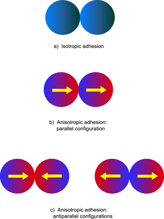
Figure 1: (Color online) Illustration of the dipolar-like adhesion. In the top panel a) the adhesion is isotropic, with $\epsilon(1,2)=1$. In the two other cases the adhesion is anisotropic and: i) stronger and maximum in the head-to-tail parallel configuration b), where $\epsilon(1,2)=1+2\alpha$; ii) weaker and minimum in the two antiparallel configurations c) ( head-to-head and tail-to-tail orientations, both with $\epsilon(1,2)=1-2\alpha$).

In the present paper we consider a ‘dipolar-like’ SHS model, where the sum of a uniform surface adhesion (isotropic background) plus an appropriate dipolar sticky correction – which can be both positive or negative, depending on the orientations of the particles – yields a nonuniform adhesion. Although the adhesion varies continuously and no discontinuous boundary exists, the surface of each molecule may be regarded as formed by two hemispherical ‘patches’ (colored red and blue, respectively, in the online Figure 1). One of these hemispheres is ‘stickier’ than the other, and the entire molecular surface is adhesive, but its stickiness is nonuniform and varies in a dipolar fashion. By varying the dipolar contribution, the degree of anisotropy can be changed, in such a way that the total sticky potential can be continuously tuned from very strong attractive strength (twice the isotropic one) to vanishing adhesion (HS limit). The physical origin of this model may be manifold (non-uniform distribution of surface charges, or hydrophobic attraction, or other physical mechanisms), one simple realization being as due to an ‘extremely screened’ attraction. The presence of a solvent together with a dense ionic atmosphere could induce any electrostatic interaction to vanish close to the molecular surface, and – in the idealized sticky limit – to become truncated exactly at contact.

For this model, we solve analytically the molecular Ornstein-Zernike (OZ) integral equation, by using a truncated Percus-Yevick (PY) approximation, with orientational linearization (PY-OL), since it retains only the lowest order terms in the expansions of the correlation functions in angular basis functions. This already provides a clear indication of the effects of anisotropy on the adhesive adhesion.

The idea of an anisotropic surface adhesion is not new. In a series of papers on hydrogen-bonded fluids such a water, Blum and co-workers Cummings86 ; Wei88 ; Blum90 already studied models of spherical molecules with anisotropic pair potentials, including both electrostatic multipolar interactions and sticky adhesive terms of multipolar symmetry. Within appropriate closures, these authors outlined the general features of the analytic solutions of the OZ equation by employing a very powerful formalism based upon expansions in rotational invariants. In particular, Blum, Cummings and Bratko Blum90 obtained an analytic solution within a mixed MSA/PY closure (extended to mixtures by Protsykevich Protsykevich03 ) for molecules which have surface adhesion of dipolar symmetry and at most dipole-dipole interactions. From the physical point of view, our model – with ‘dipolar-like’ adhesion resulting from the sum of an isotropic plus a dipolar term – is different and more specifically characterized with respect to the one of Ref. [32], whose adhesion has a simpler, strictly ‘dipolar’, symmetry. From the mathematical point of view, however, the same formalism employed by Blum et al. Blum90 could also be applied to our model. Unfortunately, the solution given in Ref. [32] is not immediately usable for the actual computation of correlation functions, since the explicit determination of the parameters involved in their analytical expressions is lacking.

In the present paper we adopt a simpler solution method, by extending the elegant approach devised by Wertheim for DHS within the MSA closure Wertheim71 , and, most importantly, we aim at providing a complete analytic solution – including the determination of all required parameters – within our PY-OL approximation.

The paper is organized as follows. Section II defines the model. In Section III we recall the molecular OZ integral equation and the basic formalism. In Section IV we present the analytic solution. Numerical exact results for some necessary parameters, as well as very accurate analytic approximations for them, will be shown in Section V. Some preliminary plots illustrating the effects of the anysotropic adhesion on the local structure are reported in Section VI. Phase stability is breafly discussed in Section VII, while final remarks and conclusions are offered in Section VIII.

II HARD SPHERES WITH ADHESION OF DIPOLAR-LIKE SYMMETRY

Let the symbol $i\equiv\left(\mathbf{r}_{i},\Omega_{i}\right)$ (with $i=1,2,3,\ldots$) denote both the position $\mathbf{r}_{i}$ of the molecular centre and the orientation $\Omega_{i}$ of molecule $i$; for linear molecules, $\Omega_{i}\equiv\left(\theta_{i},\varphi_{i}\right)$ includes the usual polar and azimuthal angles. Translational invariance for uniform fluids allows to write the dependence of the pair correlation function $g\left(1,2\right)$ as

$$(1,2)=(\mathbf{r}_{12},\Omega_{1},\Omega_{2})=(r,\Omega_{1},\Omega_{2},\widehat{\mathbf{r}}_{12})=(r,\Omega_{1},\Omega_{2},\Omega_{r}),$$

with $\mathbf{r}_{12}=\mathbf{r}_{2}-\mathbf{r}_{1}$, $r=|\mathbf{r}_{12}|$, and $\Omega_{r}$ being the solid angle associated with $\widehat{\mathbf{r}}_{12}=\mathbf{r}_{12}/r.$

In the spirit of Baxter’s isotropic counterpart Baxter68 ; Gazzillo04 , our model is defined by the Mayer function given by

$$f^{\mathrm{SHS}}(1,2)=f^{\mathrm{HS}}(r)+t\ \epsilon(1,2)\ \sigma\delta\left(r-\sigma\right),$$ (1)

where $f^{\mathrm{HS}}(r)=\Theta\left(r-\sigma\right)-1$ is its HS counterpart, $\Theta$ is the Heaviside step function ($\Theta(x<0)=0$, $\Theta(x>0)=1$) and $\delta\left(r-\sigma\right)$ the Dirac delta function, which ensures that the adhesive interaction occurs only at contact ($\sigma$ being the hard sphere diameter). An appropriate limit of the following particular square well potential of width $R-\sigma$

$$\Phi^{\mathrm{SW}}\left(1,2\right)=\left\{\begin{array}[]{ccc}+\infty\text{ \ \ \ \ \ \ \ \ \ \ \ \ \ \ \ \ \ \ \ \ \ \ \ \ \ \ \ \ \ \ \ \ \ \ }&&0<r<\sigma\\ -k_{B}T\ \ln\left[1+t\ \epsilon(1,2)\ \frac{\sigma}{R-\sigma}\ \ \right]&&\sigma<r<R\\ 0\text{ \ \ \ \ \ \ \ \ \ \ \ \ \ \ \ \ \ \ \ \ \ \ \ \ \ \ \ \ \ \ \ \ \ \ \ \ \ }&&\text{ \ \ \ \ \ \ \ }r>R\text{ ,}\end{array}\right.$$

can be shown to lead to Eq. (1).

The angular dependence is buried in the angular factor

$$\epsilon(1,2)=1+\alpha D(1,2),$$ (2)

including the dipolar function

$$D(1,2)=D(\Omega_{1},\Omega_{2},\Omega_{r})=3(\mathbf{u}_{1}\cdot\hat{\mathbf{r}})(\mathbf{u}_{2}\cdot\hat{\mathbf{r}})-\mathbf{u}_{1}\cdot\mathbf{u}_{2}$$

which stems from the dipole-dipole potential $\phi^{\mathrm{dip-dip}}(1,2)=-\mu^{2}D(1,2)/r^{3}$ ($\mu$ is the magnitude of the dipole moment) and is multiplied by the tunable anisotropy parameter $\alpha$. In the isotropic case, $\alpha=0$, one has $\epsilon(1,2)=1$. Here and in the following, $\hat{\mathbf{r}}$ coincides with $\hat{\mathbf{r}}_{12}=-\hat{\mathbf{r}}_{21}$ , while $\mathbf{u}_{i\text{ }}$is the versor attached to molecule $i$ (drawn as yellow arrow in Figure 1) which completely determines its orientation $\Omega_{i}$. Note the symmetry $D(2,1)=D(1,2)$.

The condition $\epsilon(1,2)\geq 0$ must be enforced in order to preserve a correct definition of the sticky limit, ensuring that the total sticky interaction remains attractive for all orientations, and the range of variability $-2\leq D(1,2)\leq 2$ yields the limitation $0\leq\alpha\leq\frac{1}{2}$ on the anisotropy degree. The stickiness parameter $t$ – equal to $\left(12\tau\right)^{-1}$ in Baxter’s original notation Baxter68 – measures the strength of surface adhesion relatively to the thermal energy $k_{B}T$ ($k_{B}$ being the Boltzmann constant, $T$ the absolute temperature) and increases with decreasing temperature.

If we adopt an ‘inter-molecular reference frame’ (with both polar axis and cartesian $z$-axis taken along $\mathbf{r}_{12}$), then the cartesian components of $\hat{\mathbf{r}}$ and $\mathbf{u}_{i}$ are $(0,0,1)$ and $(\sin\theta_{i}\cos\varphi_{i}$, $\sin\theta_{i}\sin\varphi_{i}$, $\cos\theta_{i})$, respectively, and thus

$$D(1,2)=2\cos\theta_{1}\cos\theta_{2}-\sin\theta_{1}\sin\theta_{2}\cos\left(\varphi_{1}-\varphi_{2}\right).$$ (3)

The strength of adhesion between two particles $1$ and $2$ at contact depends – in a continuous way – on the relative orientation of $\mathbf{u}_{1}$ and $\mathbf{u}_{2}$ as well as on the versor $\widehat{\mathbf{r}}_{12}$ of the intermolecular distance. We shall call parallel any configuration with $\mathbf{u}_{1}\cdot\mathbf{u}_{2}=1$, while antiparallel configurations are those with $\mathbf{u}_{1}\cdot\mathbf{u}_{2}=-1$ (see Figure 1). For all configurations with $D(1,2)>0$, the anisotropic part of adhesion is attractive and adds to the isotropic one. Thus, the surface adhesion is maximum, and larger than in the isotropic case, when $\mathbf{u}_{1}=\mathbf{u}_{2}=$ $\widehat{\mathbf{r}}_{12}$ and thus $\epsilon(1,2)=1+2\alpha$ (head-to-tail parallel configuration, shown in Figure 1b). On the contrary, when $D(1,2)<0$ the anisotropic contribution is repulsive and subtracts from the isotropic one, so that the total sticky interaction still remains attractive. Then, the stickiness is minimum, and may even vanish for $\alpha=1/2$, when $\mathbf{u}_{1\text{ }}=-$ $\mathbf{u}_{2}=\widehat{\mathbf{r}}_{12}$ and thus $\epsilon(1,2)=1-2\alpha$ (head-to-head or tail-to-tail antiparallel configurations, reported in Figure 1c). The intermediate case of orthogonal configuration ($\mathbf{u}_{2}$ perpendicolar to $\mathbf{u}_{1}$) corresponds to $D(1,2)=0,$ which is equivalent to the isotropic SHS interaction.

It proves convenient to ‘split’ $f^{\mathrm{SHS}}(1,2)$ as

$$\text{\ }f^{\mathrm{SHS}}(1,2)=f_{0}(r)+f_{\mathrm{ex}}(1,2),$$ (4)

$$\left\{\begin{array}[]{c}f_{0}(r)=f^{\mathrm{HS}}(r)+t\ \sigma\delta\left(r-\sigma\right)\equiv f^{\mathrm{isoSHS}}(r)\\ f_{\mathrm{ex}}(1,2)=\left(\alpha t\right)\ \sigma\delta\left(r-\sigma\right)\ D(1,2),\text{ \ \ \ \ \ \ \ \ }\end{array}\right.$$ (5)

where the spherically symmetric $f_{0}(r)$ corresponds to the ‘reference’ system with isotropic background adhesion, while $f_{\mathrm{ex}}(1,2)$ is the orientation-dependent ‘excess’ term.

We remark that, as shown in Ref. I (see also Table I in Appendix A of the present paper), convolutions of $f^{\mathrm{SHS}}$-functions generate correlation functions with a more complex angular dependence. Therefore, in addition to $D(1,2)$, it is necessary to consider also

$$\Delta(1,2)=\mathbf{u}_{1}\cdot\mathbf{u}_{2}\text{ }=\cos\theta_{1}\cos\theta_{2}+\sin\theta_{1}\sin\theta_{2}\cos\left(\varphi_{1}-\varphi_{2}\right),\$$ (6)

where the last equality holds true in the inter-molecular frame. The limits of variation for $\Delta(1,2)$ are clearly $-1\leq\Delta(1,2)\leq 1$.

III BASIC FORMALISM

This section, complemented by Appendix A, presents the main steps of  Wertheim’s formalism, as well as its extension to our model.

III.1 Molecular Ornstein-Zernike equation

The molecular OZ integral equation for a pure and homogeneous fluid of molecules interacting via non-spherical pair potentials is

$$h(1,2)=c(1,2)+\rho\int d\mathbf{r}_{3}\ \left\langle\ c(1,3)\ h(3,2)\ \right\rangle_{\Omega_{3}}\ ,$$ (7)

where $h(1,2)$ and $c(1,2)$ are the total and direct correlation functions, respectively, $\rho$ is the number density, and $g(1,2)=1+h(1,2)$ is the pair distribution function Friedman85 ; Lee88 ; Hansen06 . Moreover, the angular brackets with subscript $\Omega$ denote an average over the orientations, i.e. $\left\langle\cdots\right\rangle_{\Omega}=\left(4\pi\right)^{-1}\int d\Omega\ \cdots.$

The presence of convolution makes convenient to Fourier transform (FT) this equation, by integrating with respect to the space variable $\mathbf{r}$ alone according to

$$\widehat{F}\left(\mathbf{k},\Omega_{1},\Omega_{2}\right)=\int d\mathbf{r}\ F(\mathbf{r},\Omega_{1},\Omega_{2})\ \exp(i\mathbf{k\cdot r}).$$ (8)

The $\mathbf{r}$-space convolution becomes a product in $\mathbf{k}$-space, thus leading to

$$\widehat{h}(\mathbf{k},\Omega_{1},\Omega_{2})=\widehat{c}(\mathbf{k},\Omega_{1},\Omega_{2})+\rho\ \left\langle\widehat{c}(\mathbf{k},\Omega_{1},\Omega_{3})\ \widehat{h}(\mathbf{k},\Omega_{3},\Omega_{2})\right\rangle_{\Omega_{3}}\ .$$ (9)

As usual the OZ equation involves two unknown functions, $h$ and $c$, and can be solved only after adding a closure, that is a second (approximate) relationship among $c$, $h$ and the potential.

III.2 Splitting of the OZ equation: reference and excess part

The particular form of our potential, as defined by the Mayer function of Eq. (1), gives rise to a remarkable exact splitting of the original OZ equation. Using diagrammatic methods Friedman85 ; Lee88 ; Hansen06 it is easy to see that both $c$ and $h$ can be expressed as graphical series containing the Mayer function $f$ as bond function. If $\ f^{\mathrm{SHS}}=f_{0}+f_{\mathrm{ex}}$ is substituted into all graphs of the above series, each diagram with $n$ $f$-bonds will generate $2^{n}$ new graphs. In the cluster expansion of $c$, the sum of all graphs having only $f_{0}$-bonds will yield $c_{0}(r)=c^{\mathrm{isoSHS}}(r)$, i.e. the the direct correlation function (DCF) of the reference fluid with isotropic adhesion. On the other hand, all remaining diagrams have at least one $f_{\mathrm{ex}}$-bond, whose expression is given by Eq. (5). Thus, in the sum of this second subset of graphs it is possible to factorize $\alpha t$, and we can write

$$\text{\ }c^{\mathrm{SHS}}(1,2)=c_{0}(r)+c_{\mathrm{ex}}(1,2),$$ (10)

$$\text{ \ \ \ \ \ \ \ \ \ }\left\{\begin{array}[]{c}c_{0}(r)=c^{\mathrm{isoSHS}}(r),\text{\ \ \ \ \ \ \ \ \ \ \ \ \ \ \ \ \ \ }\\ c_{\mathrm{ex}}(1,2)=\left(\alpha t\right)\ c^{\dagger}(1,2).\text{ \ \ \ \ \ \ \ \ \ \ }\end{array}\right.$$ (11)

Similarly, for $h$ we get

$$\text{\ }h^{\mathrm{SHS}}(1,2)=h_{0}(r)+h_{\mathrm{ex}}(1,2),$$ (12)

$$\text{ \ \ \ \ \ \ \ \ \ }\left\{\begin{array}[]{c}h_{0}(r)=h^{\mathrm{isoSHS}}(r),\text{\ \ \ \ \ \ \ \ \ \ \ \ \ \ \ \ \ \ }\\ h_{\mathrm{ex}}(1,2)=\left(\alpha t\right)\ h^{\dagger}(1,2).\text{ \ \ \ \ \ \ \ \ \ \ }\end{array}\right.$$ (13)

Note that this useful separation into reference and excess part may also be extended to other correlation functions, such as $\gamma(1,2)\equiv h(1,2)-c(1,2)$, $g(1,2)=1+h(1,2)$, and the ‘cavity’ function $y(1,2)=g(1,2)/e(1,2)$. The function $\gamma$ coincides with the OZ convolution integral, without singular $\delta$-terms. Similarly $y$ is also ‘regular’, and its exact expression reads $y\left(1,2\right)=\exp\left[\ \gamma\left(1,2\right)+B(1,2)\ \right]$, where the ‘bridge’ function $B$ is defined by a complicated cluster expansion Friedman85 ; Lee88 ; Hansen06 .

From Eqs. (10)-(13), which are merely a consequence of the particular form of $f_{\mathrm{ex}}$ in the splitting of $f^{\mathrm{SHS}}$, one immediately sees that, if the anisotropy degree $\alpha$ tends to zero, then

$$\lim_{\alpha\rightarrow 0}c_{\mathrm{ex}}(1,2)=\lim_{\alpha\rightarrow 0}h_{\mathrm{ex}}(1,2)=\lim_{\alpha\rightarrow 0}y_{\mathrm{ex}}(1,2)=0.$$ (14)

Note that the spherically symmetric parts $c_{0}$ and $h_{0}$ must be related through the OZ equation for the reference fluid with isotropic adhesion (reference OZ equation)

$$h_{0}(r)=c_{0}(r)+\rho\int d\mathbf{r}_{3}\ c_{0}(r_{13})\ h_{0}(r_{32}).\$$ (15)

Thus, substituting $c$ and $h$ of Eq. (7) with $c_{0}+c_{\mathrm{ex}}$ and $h_{0}+h_{\mathrm{ex}}$, respectively, and subtracting Eq. (15), we find that $c_{\mathrm{ex}}$ and $h_{\mathrm{ex}}$ must obey the following relation

$$h_{\mathrm{ex}}(1,2) = c_{\mathrm{ex}}(1,2)+\rho\int d\mathbf{r}_{3}\ \left[\ c_{0}(r_{13})\ \left\langle\ h_{\mathrm{ex}}(3,2)\ \right\rangle_{\Omega_{3}}\right.$$

$$\left.+\left\langle\ c_{\mathrm{ex}}(1,3)\ \right\rangle_{\Omega_{3}}h_{0}(r_{32})+\left\langle\ c_{\mathrm{ex}}(1,3)\ h_{\mathrm{ex}}(3,2)\ \right\rangle_{\Omega_{3}}\ \right]\ .$$

and when

$$\left\langle\ c_{\mathrm{ex}}(1,3)\ \right\rangle_{\Omega_{3}}=\left\langle\ h_{\mathrm{ex}}(3,2)\ \right\rangle_{\Omega_{3}}=0$$ (16)

the orientation-dependent excess parts $c_{\mathrm{ex}}$ and $h_{\mathrm{ex}}$ satisfy the equality

$$h_{\mathrm{ex}}(1,2)=c_{\mathrm{ex}}(1,2)+\rho\int d\mathbf{r}_{3}\ \left\langle\ c_{\mathrm{ex}}(1,3)\ h_{\mathrm{ex}}(3,2)\ \right\rangle_{\Omega_{3}}\ ,$$ (17)

which is decoupled from that of the reference fluid and may be regarded as an OZ equation for the excess part (excess OZ equation). As we shall see, condition (16) is satisfied in our scheme.

We stress that, in principle, the closures for Eq. (15) and Eq. (17), respectively, might be different. In addition, although the two OZ equations are decoupled, a suitably selected closure might establish a relationship between $F_{0}$ and $F$ $(F=c,h).$

III.3 Percus-Yevick closure with orientational linearization

For hard-core fluids, $h$ and $c$ inside the core are given by

$$\left\{\begin{array}[]{ccc}h(1,2)=-1\text{ \ \ \ \ \ \ \ \ \ \ \ \ \ }&&\text{for \ }0<r<\sigma,\\ c(1,2)=-\left[1+\gamma(1,2)\right]&&\text{ for \ }0<r<\sigma.\end{array}\right.$$ (18)

At the same time, we have the following exact relations

$$h(1,2) = g(1,2)-1=e(1,2)y\left(1,2\right)-1,$$

$$c(1,2) = f(1,2)\left[1+\gamma(1,2)\right]+e(1,2)\left[y\left(1,2\right)-1-\gamma(1,2)\right].$$

Since $c$, $h$ and $g$ are discontinuous for hard-core fluids and involve $\delta$-terms for sticky particles, it is more convenient to define closures in terms of $y$ and $\gamma$, which are still continuous and without $\delta$-singularities. The Percus-Yevick approximation for molecular fluids with orientation-dependent interactions corresponds to assuming

$$y^{\mathrm{PY}}\left(1,2\right)=1+\gamma(1,2)\text{ \ \ \ everywhere,}$$ (19)

and thus, for the DCF,

$$c^{\mathrm{PY}}\left(1,2\right)=f(1,2)\ \left[\ 1+\gamma(1,2)\ \right]\text{,}$$ (20)

which implies that $c$ vanishes beyond the range of the potential.

However, the dependence of $\gamma(1,2)$ on angles may still be very complex. A possible procedure is to perform a series expansion of all correlation functions in terms of an infinite set of rotational invariants, which are angular basis functions – related to the spherical harmonics – having the property of rotational invariance valid for homogeneous fluids Blum71 . Unfortunately, the full PY approximation requires an infinite number of expansion coefficients for both $c(1,2)$ and $h(1,2)$. This approach is usually impracticable, but sometimes even unnecessary, as it is possible that the most significant angular basis functions are included in a small closed subset of that infinite set. Indeed this happens, for instance, in the DHS model within the MSA Wertheim71 , where the set $\{1,\Delta,D\}$ is the required subset. Although this does not happen in our model, we shall argue that the same truncation is sufficient due to the dipolar symmetry of the anisotropic adhesion.

Indeed, a natural assumption is that the only nonzero harmonics in $c(1,2)$ and $h(1,2)$ are those contained in $f(1,2)$ and those which can be obtained from that set by convolution Cummings86 . Now, the angular basis functions included in our $f$-bond are only $1$ and $D$, but the convolution of two $f$-bonds involves the angular average of two $D^{\prime}$s, which yields Wertheim71

$$\ \left\langle\ D(\mathbf{k},\Omega_{1},\Omega_{3})\ D(\mathbf{k},\Omega_{3},\Omega_{2})\ \right\rangle_{\Omega_{3}}=\frac{1}{3}\left[D(\mathbf{k},\Omega_{1},\Omega_{2})+2\Delta(\mathbf{k},\Omega_{1},\Omega_{2})\right]$$

in $\mathbf{k}$-space, and thus generates also $\Delta$. Consequently, we will expand any angle-dependent correlation function $F$ as

$$F(1,2)=F_{0}(r)+F_{\Delta}(r)\Delta(1,2)+F_{D}(r)D(1,2)+\cdots\ ,$$ (21)

neglecting all higher order terms. In other words, we assume that all angular series expansions can be truncated after these first three terms, linear with respect to the angular basis functions. Using this spirit in the PY approximation, given by Eq. (20), we obtain the following PY correlation functions with orientational linearization (OL):

$$c^{\mathrm{PY-OL}}(1,2) = c_{0}(r)+c_{\Delta}(r)\Delta(1,2)+c_{D}(r)D(1,2)$$ (22)

$$= c_{0}(r)+\left(\alpha t\right)\ \left[\ c_{\Delta}^{\dagger}(r)\Delta(1,2)+c_{D}^{\dagger}(r)D(1,2)\ \right],$$

and

$$h^{\mathrm{PY-OL}}(1,2) = h_{0}(r)+h_{\Delta}(r)\Delta(1,2)+h_{D}(r)D(1,2)$$ (23)

$$= h_{0}(r)+\left(\alpha t\right)\ \left[\ h_{\Delta}^{\dagger}(r)\Delta(1,2)+h_{D}^{\dagger}(r)D(1,2)\ \right].$$

where

$$\left.\begin{array}[]{c}c_{0}(r)=\Lambda_{0}\text{\ }\sigma\delta\left(r-\sigma\right)\\ c_{\Delta}(r)=\Lambda_{\Delta}\text{\ }\sigma\delta\left(r-\sigma\right)\\ c_{D}(r)=\Lambda_{D}\ \sigma\delta\left(r-\sigma\right)\end{array}\right\}\qquad\text{for \ }r\geq\sigma,$$ (24)

with

$$\text{\ \ }\left\{\begin{array}[]{l}\Lambda_{0}=y_{0}^{\mathrm{PY}}(\sigma)\ t\text{\ \ \ \ \ \ \ \ \ \ \ \ \ \ \ \ \ \ }\\ \Lambda_{\Delta}=y_{\Delta}^{\mathrm{PY}}(\sigma)\ t\text{\ \ \ \ \ \ \ \ \ \ \ \ \ \ \ \ \ \ }\\ \Lambda_{D}=\left[\ y_{D}^{\mathrm{PY}}(\sigma)+\alpha\ y_{0}^{\mathrm{PY}}(\sigma)\right]\ t=y_{D}^{\mathrm{PY}}(\sigma)\ t+\alpha\ \Lambda_{0},\end{array}\right.$$ (25)

$$\left\{\begin{array}[]{c}y_{0}^{\mathrm{PY}}\left(r\right)=1+\gamma_{0}(r)\text{\ \ \ \ \ \ \ \ \ \ \ \ \ \ \ \ \ }\\ y_{\Delta}^{\mathrm{PY}}(r)=\gamma_{\Delta}(r)=\left(\alpha t\right)\ y_{\Delta}^{\dagger}(r)\text{ \ \ }\\ y_{D}^{\mathrm{PY}}(r)=\gamma_{D}(r)=\left(\alpha t\right)\ y_{D}^{\dagger}(r).\text{ \ }\end{array}\right.$$ (26)

Clearly for $f(1,2)$ no truncation is required, as the expansion

$$\left\{\begin{array}[]{c}f_{0}(r)=f^{\mathrm{isoSHS}}(r)=f^{\mathrm{HS}}(r)+t\text{\ }\sigma\delta\left(r-\sigma\right)\text{\ \ \ \ \ \ \ \ \ }\\ f_{\Delta}(r)=0\text{ \ \ \ \ \ \ \ \ \ \ \ \ \ \ \ \ \ \ \ \ \ \ \ \ \ \ \ \ \ \ \ \ \ \ \ \ \ \ \ \ \ \ \ \ \ \ \ \ \ \ \ }\\ f_{D}(r)=\left(\alpha t\right)\ \sigma\delta\left(r-\sigma\right)\text{ \ \ \ \ \ \ \ \ \ \ \ \ \ \ \ \ \ \ \ \ \ \ \ \ \ \ \ \ \ \ \ \ }\end{array}\right.$$ (27)

is exact.

It can be shown that $c(1,2)$ and $h(1,2)$ must have the same approximate form in view of the OZ equation, Eq. (7).

The solution of the original OZ equation (7) is then equivalent to the calculation of the radial coefficients $c_{0}(r),c_{\Delta}(r),c_{D}(r)$ and $h_{0}(r),h_{\Delta}(r),h_{D}(r)$, which are the projections of $c(1,2)$ and $h(1,2)$ onto the angular basis $\left\{1,\Delta,D\right\}$. The core condition on $h$, Eq. (18), becomes

$$\left.\begin{array}[]{c}h_{0}(r)=-1\\ h_{\Delta}(r)=0\\ h_{D}(r)=0\end{array}\right\}\text{ \ \ \ \ \ for \ }0<r<\sigma.$$ (28)

Note that in the zero density limit $\gamma(1,2)=\rho\int d\mathbf{r}_{3}\ \left\langle\ c(1,3)\ h(3,2)\ \right\rangle_{\Omega_{3}}$ must vanish, and thus $y^{\mathrm{PY}}(1,2)\rightarrow 1$, i.e.

$$\lim_{\rho\rightarrow 0}y_{0}^{\mathrm{PY}}(r)=1\text{, \ \ \ \ \ \ \ }\lim_{\rho\rightarrow 0}y_{\Delta}^{\mathrm{PY}}(r)=\lim_{\rho\rightarrow 0}y_{D}^{\mathrm{PY}}(r)=0,$$

while both $c\left(1,2\right)$ and $h\left(1,2\right)$ must reduce to $f(1,2)$:

$$\begin{array}[]{c}\lim_{\rho\rightarrow 0}F_{0}(r)=f_{0}(r)\text{ }\\ \text{\ }\lim_{\rho\rightarrow 0}F_{\Delta}(r)=0\text{ \ \ \ \ \ \ \ }\\ \lim_{\rho\rightarrow 0}F_{D}(r)=f_{D}(r)\text{ }\end{array}\text{\ \ \ \ \ \ }(F=c,h),$$

and

$$\lim_{\rho\rightarrow 0}\Lambda_{0}=t\text{, \ \ \ \ \ \ \ }\lim_{\rho\rightarrow 0}\Lambda_{\Delta}=0\text{, \ \ \ \ \ \ }\lim_{\rho\rightarrow 0}\Lambda_{D}=\alpha t\text{.}$$ (29)

Moreover as $\alpha\rightarrow 0$ all $\Delta$- and $D$-coefficients of $c,h$ and $y$ vanish, so that the isotropic adhesion case is recovered. Finally, it is also worth stressing that the same $\delta$-term arises in $c,$ $h$ and $g$, that is

$$F(1,2)=F_{\mathrm{reg}}(1,2)+F_{\text{sing}}(1,2)\text{ \ \ \ \ \ \ (}F=c,h,g),$$

where $F_{\mathrm{reg}}$ is the ‘regular’ part (i.e., the part with no $\delta$-singularity, and – at most – some step discontinuities), while $F_{\text{sing}}(1,2)=\ \sigma\delta\left(r-\sigma\right)\Lambda(1,2)$ is the singular term representing the anisotropic surface adhesion ( with$\ \Lambda(1,2)=\Lambda_{0}+\Lambda_{\Delta}\Delta(1,2)+\Lambda_{D}D(1,2)$  ).

III.4 Integral equations for the projections of $c$ and $h$

In the following, we extend Wertheim theory Wertheim71 to our model, in order to obtain the radial projections of $c$ and $h$.

The PY-OL approximation to the excess anisotropic part of the correlation functions is

$$\begin{array}[]{c}c_{\mathrm{ex}}^{\mathrm{PY-OL}}(1,2)=c_{\Delta}(r)\Delta(1,2)+c_{D}(r)D(1,2)\text{ }\\ h_{\mathrm{ex}}^{\mathrm{PY-OL}}(1,2)=h_{\Delta}(r)\Delta(1,2)+h_{D}(r)D(1,2),\end{array}$$ (30)

thus verifying the required property $\left\langle\ c_{\mathrm{ex}}(1,3)\ \right\rangle_{\Omega_{3}}=\left\langle\ h_{\mathrm{ex}}(3,2)\ \right\rangle_{\Omega_{3}}=0$ described in Section III, and allowing the splitting of the molecular OZ equation into a reference and an excess part.

The first part is the reference PY equation, and coincides with that solved by Baxter for the fluid with isotropic adhesion Baxter68 ; Baxter71 :

$$\left\{\begin{array}[]{cc}h_{0}(r)=c_{0}(r)+\rho\ (h_{0}\star c_{0})\text{ \ \ \ \ \ \ \ \ \ \ \ \ \ \ \ }&\\ h_{0}(r)=-1\text{\ \ \ \ \ \ \ \ \ \ \ \ \ \ \ \ \ \ \ \ \ \ \ \ \ \ \ \ \ \ \ \ \ \ \ }&0<r<\sigma\\ c_{0}(r)=\Lambda_{0}\ \sigma\delta\left(r-\sigma\right)\text{ \ \ \ \ \ \ \ \ \ \ \ \ \ \ \ \ \ \ \ \ }&r\geq\sigma,\end{array}\right.$$ (31)

where the symbol $\star$ denotes spatial convolution, i.e. $(A\star B)(r_{12})=\int A(r_{13})B(r_{32})\;d\mathbf{r}_{3}$.

The second part is the excess PY-OL equation, given by Eq. (17) coupled with the PY-OL closure. Following an extension of Wertheim’s approach, as described in detail in Appendix A, Eq. (17) can be splitted into the following system for the $\Delta-$ and $D-$projections of $c$ and $h:$

$$\left\{\begin{array}[]{c}h_{\Delta}(r)=c_{\Delta}(r)+\frac{1}{3}\rho~{}\left(\ c_{\Delta}\star h_{\Delta}+2\ c_{D}^{0}\star h_{D}^{0}\ \right)\text{\ \ \ \ \ \ \ \ \ \ \ }\\ h_{D}^{0}(r)=c_{D}^{0}(r)+\frac{1}{3}\rho~{}\left(\ c_{\Delta}\star h_{D}^{0}+c_{D}^{0}\star h_{\Delta}+c_{D}^{0}\star h_{D}^{0}\ \right),\end{array}\right.$$ (32)

where $c_{D}^{0}(r)$ and $h_{D}^{0}(r)$ are defined by the relationship

$$F_{D}^{0}(r)=F_{D}(r)-3\int_{r}^{\infty}\frac{F_{D}(x)}{x}\ dx\text{ \ \ \ \ \ \ \ \ }(F=c,h),$$ (33)

whose inverse is Wertheim71

$$F_{D}(r)=F_{D}^{0}(r)-\frac{3}{r^{3}}\int_{0}^{r}F_{D}^{0}(x)\ x^{2}\ dx.$$ (34)

The core conditions become

$$\left.\begin{array}[]{c}\text{ \ }h_{\Delta}(r)=0\text{ \ \ \ \ \ \ }\\ h_{D}^{0}(r)=-3K\end{array}\right\}\text{ \ \ \ \ \ for \ }0<r<\sigma,$$ (35)

with

$$K=\int_{\sigma^{-}}^{\infty}\frac{h_{D}(x)}{x}\ dx=K_{\mathrm{reg}}+\Lambda_{D}\ ,$$ (36)

$$K_{\mathrm{reg}}=\int_{\sigma}^{\infty}\frac{h_{D,\text{{reg}}}(r)}{r}\ dr.$$ (37)

Note that the presence of the $\delta$-singularity in $h_{D}(x)$ requires the specification of $\sigma^{-}$ as lower integration limit, unlike the case of Ref. I where only the regular part $K_{\mathrm{reg}}$ is present. Moreover, since $h_{D}(r)=\alpha t\ \ h_{D}^{\dagger}(r)$, from Eq. (36) one could also write

$$K=\alpha t\ \mathcal{K}\text{ ,}$$ (38)

which shows that $K$ is related to the anisotropy degree, and vanishes both in the symmetric adhesion case ($\alpha=0$) and in the HS limit ($t=0$). Since $h_{D}(r)\rightarrow f_{D}(r)=\left(\alpha t\right)\sigma\delta(r-\sigma)$ in the zero density limit, one then finds that

$$\lim_{\eta\rightarrow 0}K=\alpha t.$$ (39)

Finally, the PY-OL closure for the new DCFs reads

$$\left.\begin{array}[]{c}c_{\Delta}(r)=\Lambda_{\Delta}\ \sigma\delta\left(r-\sigma\right)\\ c_{D}^{0}(r)=\Lambda_{D}\ \sigma\delta\left(r-\sigma\right)\end{array}\right\}\text{ \ \ \ \ \ }r\geq\sigma$$ (40)

(for simplicity, here and in the following we omit the superscript PY-OL).

III.5 Decoupling of the integral equations

It is possible to decouple the two equations for $\Delta$- and $D$-coefficients, by introducing two new unknown functions, which are linear combinations of the previous ones. As shown in Appendix A, if we define $F_{1}(r)$ and $F_{2}(r)$ $\left(F=c,h\right)$ through the relations

$$\left\{\begin{array}[]{c}F_{1}\left(r\right)=\left(3\mathcal{L}_{1}\right)^{-1}\left[F_{\Delta}(r)-F_{D}^{0}(r)\right]\text{ }\\ F_{2}\left(r\right)=\left(3\mathcal{L}_{2}\right)^{-1}\left[F_{\Delta}(r)+2F_{D}^{0}(r)\right]\end{array}\right.\text{\ \ \ \ }\left(F=c,h\right),$$

then we get the OZ equations

$$\left\{\begin{array}[]{c}h_{1}(r)=c_{1}(r)+\rho_{1}\ (h_{1}\star c_{1})\text{ }\\ h_{2}(r)=c_{2}(r)+\rho_{2}\ (h_{2}\star c_{2}),\end{array}\right.$$

with the following densities and core conditions

$$\left\{\begin{array}[]{c}\rho_{1}=\mathcal{L}_{1}\ \rho\text{ }\\ \rho_{2}=\mathcal{L}_{2}\ \rho,\end{array}\right.\qquad\qquad\left\{\begin{array}[]{c}h_{1}(r)=K/\mathcal{L}_{1}\text{ \ \ \ }\\ h_{2}(r)=-2K/\mathcal{L}_{2}\end{array}\right.\text{ \ \ \ \ \ for \ }0<r<\sigma.$$

The decoupling of the three different projections of $c$ and $h$ is remarkable: the molecular anisotropic OZ equation reduces to a set of three radial integral relations, which may be regarded as OZ equations for three ‘hypothetical’ fluids (labelled as $0,1,2$) with spherically symmetric interactions. We stress that there is not a unique solution to the decoupling problem, since - in principle - there exist infinite possible choices for $\left(\mathcal{L}_{1},\mathcal{L}_{2}\right)$. The final results are clearly independent of the values of $\left(\mathcal{L}_{1},\mathcal{L}_{2}\right)$.

In the present paper, we adopt Wertheim’s choice, i.e. $\mathcal{L}_{1}=-K$ and $\mathcal{L}_{2}=2K$, which leads to

$$\left\{\begin{array}[]{c}F_{1}\left(r\right)=\frac{1}{3K}\left[F_{D}^{0}(r)-F_{\Delta}(r)\right]\text{ }\\ F_{2}\left(r\right)=\frac{1}{3K}\left[F_{D}^{0}(r)+\frac{1}{2}F_{\Delta}(r)\right]\end{array}\right.\text{\ \ \ \ }\left(F=c,h\right),$$ (41)

$$\left\{\begin{array}[]{c}\rho_{1}=-K\rho\text{ }\\ \rho_{2}=2K\rho,\end{array}\right.\qquad\qquad\left\{\begin{array}[]{c}h_{1}(r)=-1\\ h_{2}(r)=-1\end{array}\right.\text{ \ \ \ \ \ for \ }0<r<\sigma$$ (42)

(in Ref. I, $F_{1}$ and $F_{2}$ were denoted as $F_{-}$ and $F_{+}$, respectively).

Note that the auxiliary fluids have densities different from that of the reference fluid (the negative sign of $\rho_{1}$ poses no special difficulty).

We can also write

$$F_{m}\left(r\right)=F_{m,\mathrm{reg}}(r)+\Lambda_{m}\ \sigma\delta\left(r-\sigma\right),$$ (43)

with

$$\left\{\begin{array}[]{c}F_{1,\mathrm{reg}}\left(r\right)=\frac{1}{3K}\left[F_{D,\mathrm{reg}}^{0}(r)-F_{\Delta,\mathrm{reg}}(r)\right]\text{ }\\ F_{2,\mathrm{reg}}\left(r\right)=\frac{1}{3K}\left[F_{D,\mathrm{reg}}^{0}(r)+\frac{1}{2}F_{\Delta,\mathrm{reg}}(r)\right]\end{array}\right.$$ (44)

and

$$\left\{\begin{array}[]{c}\Lambda_{1}=\frac{1}{3K}\left(\Lambda_{D}-\Lambda_{\Delta}\text{\ }\right)\text{ \ \ \ \ \ \ \ \ \ \ \ \ \ \ \ \ \ \ \ \ \ \ \ \ \ \ \ \ \ \ \ \ \ \ \ \ \ \ \ }\\ =\frac{1}{3K}\left[h_{D,\text{{reg}}}(\sigma^{+})-h_{\Delta,\text{{reg}}}(\sigma^{+})\right]\ t\text{ }+\alpha\ \frac{1}{3K}\ \Lambda_{0}\text{ \ }\\ \text{\ \ \ \ \ \ }\\ \Lambda_{2}=\frac{1}{3K}\left(\Lambda_{D}+\frac{1}{2}\Lambda_{\Delta}\right)\text{ \ \ \ \ \ \ \ \ \ \ \ \ \ \ \ \ \ \ \ \ \ \ \ \ \ \ \ \ \ \ \ \ \ \ \ \ \ \ }\\ \text{ \ \ }=\frac{1}{3K}\left[h_{D,\text{{reg}}}(\sigma^{+})+\frac{1}{2}h_{\Delta,\text{{reg}}}(\sigma^{+})\right]\ t\text{ }+\alpha\ \frac{1}{3K}\ \Lambda_{0}\text{.\ \ }\end{array}\right.$$ (45)

(since $\gamma_{\ldots}(\sigma)=h_{\ldots,\text{{reg}}}(\sigma^{+})-c_{\ldots,\text{{reg}}}(\sigma^{+})$, and $c_{\ldots,\text{{reg}}}(\sigma^{+})=0$ within the PY-OL closure).

Knowing the correlation functions $F_{1}(r)$ and $F_{2}(r)$ $\left(\text{with }F=c,h\right)$, one can derive $F_{\Delta}\left(r\right),F_{D}^{0}\left(r\right)$, i.e.

$$\left\{\begin{array}[]{c}F_{\Delta}\left(r\right)=2K\left[F_{2}\left(r\right)-F_{1}\left(r\right)\right]\ \text{\ \ \ \ }\\ F_{D}^{0}\left(r\right)=2K\left[F_{2}\left(r\right)+\frac{1}{2}F_{1}\left(r\right)\right]\ ,\end{array}\right.$$ (46)

and

$$\left\{\begin{array}[]{c}\Lambda_{\Delta}=2K\left(\Lambda_{2}-\Lambda_{1}\right)\text{\ \ \ \ }\\ \Lambda_{D}=K\left(2\Lambda_{2}+\Lambda_{1}\right)\text{ .\ \ }\end{array}\right.$$ (47)

Finally, from $F_{\Delta}\left(r\right),F_{D}^{0}\left(r\right)$ one has to evaluate $F_{\Delta}\left(r\right),F_{D}\left(r\right)$, by employing Eq. (34). We note the following points:

i) Insertion of $h_{D}^{0}(r)=h_{D,\text{{reg}}}^{0}(r)+\Lambda_{D}\ \sigma\delta(r-\sigma)$ into Eq. (34) yields $h_{D}(r)=h_{D,\text{{reg}}}(r)+\Lambda_{D}\ \sigma\delta(r-\sigma),$ with

$$h_{D,\text{{reg}}}(r)=\left\{\begin{array}[]{cc}0\text{ \ \ \ \ \ \ \ \ \ \ \ \ \ \ \ \ \ \ \ \ \ \ \ \ \ \ \ \ \ \ \ \ \ \ \ \ \ \ \ \ \ \ \ \ \ }0<r<\sigma,\text{\ \ \ \ \ \ }&\\ h_{D,\text{{reg}}}^{0}(r)+3r^{-3}\left[K_{\mathrm{reg}}\sigma^{3}-\int_{\sigma}^{r}h_{D,\text{{reg}}}^{0}(x)\ x^{2}\ dx\right]\text{ \ \ \ \ \ \ \ }&r>\sigma.\end{array}\right.$$ (48)

At $r=2\sigma$ $h_{D,\text{{reg}}}$ and $h_{D,\text{{reg}}}^{0}$ have the same discontinuity. We also get

$$h_{D,\text{{reg}}}(\sigma^{+})=h_{D,\text{{reg}}}^{0}(\sigma^{+})+3K_{\mathrm{reg}}.$$ (49)

Clearly, these results must agree with those obtained from Eq. (33), i.e.

$$\begin{array}[]{c}h_{D}^{0}(r)=h_{D}(r)-3\psi(r),\text{ \ \ \ \ \ \ \ \ \ \ \ \ \ \ \ \ \ \ \ \ \ \ \ \ \ \ \ \ \ \ \ \ \ \ \ \ \ \ \ \ \ \ \ \ \ \ \ \ }\\ \psi(r)\equiv\int_{r}^{\infty}h_{D}(x)\ x^{-1}\ dx=\Lambda_{D}\ \theta\left(\sigma-r\right)+\int_{r}^{\infty}h_{D,\text{{reg}}}(x)\ x^{-1}\ dx.\end{array}\text{\ }$$

In order to recover Eq. (49) along this second route, note that $\psi(r)$ is not continuous at $r=\sigma$. In fact, from Eqs. (36) and (37) follows $\psi(\sigma^{-})=K$ whereas $\psi(\sigma^{+})=K_{\mathrm{reg}}.$

ii) Similarly, for $c_{D}(r)$ we obtain $c_{D}(r)=c_{D,\text{{reg}}}(r)+\Lambda_{D}\ \sigma\delta(r-\sigma)$, with

$$c_{D,\text{{reg}}}(r)=c_{D,\text{{reg}}}^{0}(r)-3r^{-3}\left[\int_{0}^{r}\ c_{D,\text{{reg}}}^{0}(x)x^{2}\ dx+\Lambda_{D}\sigma^{3}\ \theta(r-\sigma)\right],$$ (50)

since $\int_{0}^{r}\ \delta(x-\sigma)x^{2}dx=\sigma^{2}\theta(r-\sigma)$. On the other hand, from Eq. (33) one easily finds that

$$c_{D}(r)=c_{D}^{0}(r)\text{ \ \ \ for \ }r\geq\sigma.$$ (51)

iii) By applying the relationship (34) to $c_{D}(r)$, using Eq. (51) and noticing that $c_{D}(x)=0$ for $r>\sigma$ within the PY-OL approximation, leads to a sum rule:

$$\int_{0}^{\infty}c_{D}^{0}(x)\ x^{2}\ dx=\int_{0}^{\sigma}\ c_{D,\text{{reg}}}^{0}(x)x^{2}\ dx+\Lambda_{D}\sigma^{3}\ =0,$$ (52)

that we will exploit later.

IV ANALYTIC SOLUTION

We have seen that the molecular PY-OL integral equation (IE) for our anisotropic-SHS model splits into three IE’s

$$\left\{\begin{array}[]{cc}h_{m}(r)=c_{m}(r)+\rho_{m}\ (h_{m}\star c_{m})\text{\ \ }&\\ h_{m}(r)=-1\text{\ \ \ \ \ \ \ \ \ \ \ \ \ \ \ \ \ \ \ \ \ \ \ \ \ \ }&0<r<\sigma\\ c_{m}(r)=\Lambda_{m}\ \sigma\delta\left(r-\sigma\right)\text{ \ \ \ \ \ \ \ \ \ \ }&r\geq\sigma\end{array}\right.\qquad\left(m=0,1,2\right),$$ (53)

where

$$\left\{\begin{array}[]{c}\rho_{0}=\rho\text{ \ \ \ \ \ }\\ \rho_{1}=-K\rho\text{ }\\ \rho_{2}=2K\rho,\end{array}\right.$$ (54)

and the ‘amplitudes’ of the adhesive $\delta$-terms are

$$\left\{\begin{array}[]{c}\text{ }\Lambda_{0}=\left[1+h_{0,\text{{reg}}}(\sigma^{+})\right]\ t=y_{0}^{\mathrm{PY}}(\sigma)t\text{ }\text{ \ \ \ \ \ \ \ \ \ \ \ \ \ \ \ \ \ \ \ \ \ \ \ \ \ \ \ \ \ \ }\\ \text{ }\Lambda_{m}=h_{m,\text{{reg}}}(\sigma^{+})\ t\text{ }+\mathcal{P}=y_{m}^{\mathrm{PY}}(\sigma)t+\mathcal{P}\text{ \ \ \ \ \ }\left(m=1,2\right),\text{ }\end{array}\right.$$ (55)

with

$$\mathcal{P}=\frac{1}{3}\ \frac{\alpha t\ y_{0}^{\mathrm{PY}}(\sigma)\ }{K}+\frac{K_{\mathrm{reg}}}{K}\ t=\frac{1}{3}\ \frac{\alpha\ \Lambda_{0}\ }{K}+\frac{K_{\mathrm{reg}}}{K}\ t.$$ (56)

Here, the new expressions of $\Lambda_{1}$ and $\Lambda_{2}$ have been obtained from Eqs. (45) with the help of Eqs. (49) and (44).

The essential difference with respect to Ref. I lies in the closure, which is – of course – related to the model potential. While Wertheim’s paper on DHS Wertheim71 employed the MSA closure, which performs properly for long-ranged electrostatic potentials at low strength of interaction, our PY-OL closure is more appropriate for the short-ranged potential of the present model.

The first integral equation IE0 is fully independent, whereas IE1 and IE2 depend on the solution of IE0 (unlike the case of Ref. I), because of the presence of $\Lambda_{0}$ inside $\Lambda_{1\text{ }}$and $\Lambda_{2}$. While IE0 is exactly the PY equation for the reference SHS with isotropic adhesion solved by Baxter Baxter68 ; Baxter71 , IE1 and IE2 are different from both Wertheim’s MSA solution for DHS and Baxter’s PY solution for SHS. We remark that the closures for IE1 and IE2 are not PY as $\Lambda_{1\text{ }}$and $\Lambda_{2}$ – given by Eq. (55) – differ, by the term $\mathcal{P}$, from those appropriate for the PY choice, corresponding to $\Lambda_{m}^{\mathrm{PY}}=y_{m}^{\mathrm{PY}}(\sigma)t$.

Consequently, IE1 and IE2 can be rekoned as belonging to a class of generalized PY  (GPY) approximations, introduced in Ref. [39], which admit an analytic solution. Thus, the PY-OL closure for $c(1,2)$ leads to a PY integral equation for $c_{0}(r)$, coupled to a two GPY integral equations for $c_{1}(r)$ and $c_{2}(r)$ (which are linear combinations of $c_{\Delta}(r)$ and $c_{D}^{0}(r)$).

On comparing the three IE’s and their closures given by Eq. (53), it is apparent that they have exactly the same form, but differ by the density $\rho_{m}$ and the expression for $\Lambda_{m}$. The first integral equation IE0 corresponds to an isotropic SHS fluid with density $\rho$. On the other hand, IE1 and IE2 refer to ‘auxiliary’ isotropic SHS fluids with densities $\rho_{1}$ and $\rho_{2}$, and adhesion parameters $\Lambda_{1}$ and $\Lambda_{2}$, respectively. Note that, according to Eqs. (45) , $\Lambda_{m}$ is not evaluated at the actual density $\rho_{m}$ of the auxiliary fluid, but at the real density $\rho$ . These remarks strongly suggests that the solutions of IE0, IE1 and IE2 can be expressed in terms of an unique solution – the PY one for isotropic SHS – by changing only $\rho_{m}$ and $\Lambda_{m}$. This can be achieved by the formal mapping

$$\left\{\begin{array}[]{c}F_{0}(r)=F^{\mathrm{isoSHS}}(r;\eta_{0},\Lambda_{0})\text{ }\\ F_{1}(r)=F^{\mathrm{isoSHS}}(r;\eta_{1},\Lambda_{1})\text{ }\\ F_{2}(r)=F^{\mathrm{isoSHS}}(r;\eta_{2},\Lambda_{2}),\end{array}\right.\qquad\quad(F=q,c,h)$$ (57)

where $\eta_{0}=\eta$ is the real volume fraction, while $\eta_{1}$ and $\eta_{2}$ are ‘modified volume fractions’ of the ‘auxiliary’ fluids $1$ and $2$, i.e.,

$$\left\{\begin{array}[]{c}\eta_{0}=\eta\equiv\left(\pi/6\right)\rho\sigma^{3}\text{ \ \ }\\ \eta_{1}=-K\eta\text{ \ \ \ \ \ \ \ \ \ \ \ \ \ }\\ \eta_{2}=2K\eta\text{\ .\ \ \ \ \ \ \ \ \ \ \ \ \ }\end{array}\right.$$ (58)

In Eqs. (57) $q(r)$ denotes the Baxter factor correlation function, introduced in the next Subsection.

It is worth noting that this result for SHS mirrors the analog of the MSA solution for DHS Wertheim71 where all the three harmonic coefficients of can be expressed similarly, in terms of a single PY solution for the reference HS fluid.

IV.1 Baxter factorization

We shall now solve Eqs. (53) by using the Wiener-Hopf factorization due to Baxter Baxter71 . Let us recall its basic steps. After Fourier transforming the OZ equation for a one-component fluid with spherically symmetric interactions, one assumes the following factorization:

$$\begin{array}[]{c}1-\rho\widetilde{c}\left(k\right)=Q(k)Q(-k),\\ Q(k)=1-2\pi\rho\int_{0}^{\infty}q(r)\ e^{ikr}dr.\end{array}$$ (59)

Then it can be shown that the introduction of the ‘factor correlation function’ $q(r)$ allows the OZ equation to be cast into the form Baxter71

$$\left\{\begin{array}[]{c}rc\left(r\right)=-q^{\prime}(r)+2\pi\rho\int_{0}^{\infty}du\ q\left(u\right)q^{\prime}\left(r+u\right),\text{ \ \ \ \ \ \ \ \ \ \ }\\ rh\left(r\right)=-q^{\prime}(r)+2\pi\rho\int_{0}^{\infty}du\ q\left(u\right)\left(r-u\right)h\left(|r-u|\right),\end{array}\right.$$ (60)

where the prime denotes differentiation with respect to $r$. Solving these Baxter equations is tantamount to determining – within a chosen closure – the function $q(r)$, from which $c\left(r\right)$ and $h\left(r\right)$ can be easily calculated. It is also necessary to remember that, for all closures leading to $c\left(r\right)=0$ for $r>\sigma$, one finds $q\left(r\right)=0$ for $r>\sigma$ Gazzillo04 .

On applying Baxter’s factorization to Eqs. (53), we get

$$rh_{m}\left(r\right)=-q_{m}^{\prime}(r)+2\pi\rho_{m}\int_{0}^{\sigma}du\ q_{m}\left(u\right)\left(r-u\right)h_{m}\left(|r-u|\right).$$ (61)

with $m=0,1,2$. Now the closure $c_{m}(r)=\Lambda_{m}\ \sigma\delta\left(r-\sigma\right)$ for  $r\geq\sigma$ implies that the same $\delta$-term must appear in $h_{m}\left(r\right)$. Thus, for $0\leq r\leq\sigma$, using $h_{m}(r)=-1+\Lambda_{m}\ \sigma\delta\left(r-\sigma\right)$, we find

$$q_{m}^{\prime}(r)=a_{m}r+b_{m}\sigma-\Lambda_{m}\ \sigma^{2}\delta\left(r-\sigma\right),$$

with

$$\left\{\begin{array}[]{c}a_{m}=\ 1-2\pi\rho_{m}\int_{0}^{\sigma}du\ q_{m}\left(u\right)\ ,\\ b_{m}\sigma=\ 2\pi\rho_{m}\int_{0}^{\sigma}du\ q_{m}\left(u\right)\ u\ .\text{ \ \ }\end{array}\right.$$ (62)

The $\delta$-term of $q_{m}^{\prime}(r)$ means that $q_{m}(r)$ has a discontinuity $q_{m}(\sigma^{+})-q_{m}(\sigma^{-})=-\Lambda_{m}\sigma^{2}$, with $q_{m}(\sigma^{+})=0.$ Integrating $q_{m}^{\prime}(r)$, substituting this result into Eqs. (62), and solving the corresponding algebraic system, we find the following solution

$$q_{m}(r)=\left\{\begin{array}[]{cc}\ \frac{1}{2}a_{m}(r-\sigma)^{2}+\left(a_{m}+b_{m}\right)\sigma(r-\sigma)\ +\Lambda_{m}\ \sigma^{2}&\text{ \ \ \ \ }0\leq r\leq\sigma,\\ 0&\text{ \ \ \ otherwise,}\end{array}\right.$$ (63)

$$a_{m} = \ a^{\mathrm{HS}}(\eta_{m})-\frac{12\eta_{m}\ \Lambda_{m}\ }{1-\eta_{m}}\$$ (64)

$$b_{m} = \ b^{\mathrm{HS}}(\eta_{m})+\frac{6\eta_{m}\ \Lambda_{m}\ }{1-\eta_{m}}\ \$$ (65)

$$\text{\ }\eta_{m} = \left(\pi/6\right)\rho_{m}\sigma^{3}\text{ \ \ \ }$$ (66)

$$a^{\mathrm{HS}}(x) = \frac{1+2x}{\left(1-x\right)^{2}},\text{ \ \ \ \ \ \ \ }b^{\mathrm{HS}}(x)=-\frac{3x}{2\left(1-x\right)^{2}},$$ (67)

From the first of Eqs. (60) we get the DCFs $c_{m}(r)=c_{m,\text{{reg}}}(r)+\ \Lambda_{m}\ \sigma\delta(r-\sigma)$, where $c_{m,\text{{reg}}}(r)=0$ for $r\geq\sigma,$ and for $0<r<\sigma$

$$c_{m,\text{{reg}}}(r) = -\frac{1}{2}\eta_{m}\ a_{m}^{2}\left(\frac{r}{\sigma}\right)^{3}+6\eta_{m}\ \left[\ (a_{m}+b_{m})^{2}-2a_{m}\ \Lambda_{m}\ \right]\left(\frac{r}{\sigma}\right)$$ (68)

$$-a_{m}^{2}-12\eta_{m}\ \Lambda_{m}^{2}\left(\frac{r}{\sigma}\right)^{-1}.$$

The second of Eqs. (60) yields the total correlation functions $h_{m}(r)=h_{m,\text{{reg}}}(r)+\ \Lambda_{m}\ \sigma\delta(r-\sigma).$ For $r>\sigma$, Eqs. (61) becomes

$$H_{m,\text{{reg}}}\left(r\right)=12\eta_{m}\ \sigma^{-3}\left\{\begin{array}[]{cc}\begin{array}[]{c}\int_{0}^{r-\sigma}du\ q_{m}\left(u\right)\ H_{m,\text{{reg}}}\left(r-u\right)\text{ \ \ \ \ \ \ \ \ \ \ \ \ \ \ \ \ \ \ \ \ \ \ \ \ \ \ \ \ \ \ \ }\\ +\ \int_{r-\sigma}^{\sigma}du\ q_{m}\left(u\right)\left(u-r\right)+\Lambda_{m}\sigma^{2}\ q_{m}\left(r-\sigma\right)\text{ \ \ \ }\end{array}&\sigma<r<2\sigma,\\ &\\ \int_{0}^{\sigma}du\ q_{m}\left(u\right)\ H_{m,\text{{reg}}}\left(r-u\right)\text{ \ \ \ \ \ \ \ \ \ \ \ \ \ }r>2\sigma,\text{\ \ \ \ \ \ \ \ \ \ \ }&\end{array}\right.$$ (69)

where $H_{m}\left(r\right)\equiv rh_{m}\left(r\right)$. Due to the last term of Eq. (69) and the discontinuity of $q_{m}\left(r\right)$ at $r=\sigma$, $h_{m,\text{{reg}}}(r)$ has a jump of at $r=2\sigma$ Kranendonk88 ; Miller04 : $h_{m,\text{{reg}}}(2\sigma^{+})-h_{m,\text{{reg}}}(2\sigma^{-})=-6\eta_{m}\ \Lambda_{m}^{2}.$

IV.2 An important relationship

In Appendix B it is shown that a remarkable consequence of the sum rule (52) is the condition

$$a_{2}=a_{1}\text{ ,}$$ (70)

that will play a significant role in the determination of the unknown parameters $\Lambda_{1},$ $\Lambda_{2}$ and $K$  (see Appendix B).

IV.3 Reference fluid coefficients

The $m=0$ case corresponds to Baxter’s PY results for the reference fluid of isotropic SHS particles Baxter68 ; Baxter71 . We have: $q_{0}(r)=q^{\mathrm{isoSHS}}(r;\eta,\Lambda_{0}),$ and

$$\left\{\begin{array}[]{c}c_{0}(r)=c^{\mathrm{isoSHS}}(r;\eta,\Lambda_{0})=c_{\text{{reg}}}^{\mathrm{isoSHS}}(r;\eta,\Lambda_{0})+\Lambda_{0}\ \sigma\delta(r-\sigma)\text{ }\\ h_{0}(r)=h^{\mathrm{isoSHS}}(r;\eta,\Lambda_{0})=h_{\text{{reg}}}^{\mathrm{isoSHS}}(r;\eta,\Lambda_{0})+\Lambda_{0}\ \sigma\delta(r-\sigma)\end{array}\right.$$ (71)

(for simplicity, we omit – here and in the following – the superscript PY).

IV.4 $\Delta-$ and $D-$coefficients

We write $q_{m}(r)=q^{\mathrm{isoSHS}}(r;\eta_{m},\Lambda_{m})$ with $m=1,2$. Then,

i) For the $\Delta$-coefficients, after recalling Eq. (43) and exploiting Eqs. (47), we end up with:

$$\left\{\begin{array}[]{c}c_{\Delta}(r)=2K\left[c_{0,\text{{reg}}}(r;2K\eta,\Lambda_{2})-c_{0,\text{{reg}}}(r;-K\eta,\Lambda_{1})\right]+\Lambda_{\Delta}\ \sigma\delta(r-\sigma)\text{\ \ \ }\\ h_{\Delta}(r)=2K\left[h_{0,\text{{reg}}}(r;2K\eta,\Lambda_{2})-h_{0,\text{{reg}}}(r;-K\eta,\Lambda_{1})\right]+\Lambda_{\Delta}\ \sigma\delta(r-\sigma).\text{ \ }\end{array}\right.$$ (72)

ii) For the $D$-coefficients, we get

$$\left\{\begin{array}[]{c}c_{D}^{0}(r)=2K\left[c_{0,\text{{reg}}}(r;2K\eta,\Lambda_{2})+\frac{1}{2}c_{0,\text{{reg}}}(r;-K\eta,\Lambda_{1})\right]\ +\Lambda_{D}\ \sigma\delta(r-\sigma)\text{ \ }\\ h_{D}^{0}(r)=2K\left[h_{0,\text{{reg}}}(r;2K\eta,\Lambda_{2})+\frac{1}{2}h_{0,\text{{reg}}}(r;-K\eta,\Lambda_{1})\right]\ +\Lambda_{D}\ \sigma\delta(r-\sigma).\text{ }\end{array}\right.$$ (73)

Finally, from $c_{D}^{0}(r)$ and $h_{D}^{0}(r)$ we can calculate $c_{D}(r)$ and $h_{D}(r)$, as described by Eqs. (50) and (48), respectively.

In short, a) our PY-OL solution – $\left\{c_{0},c_{\Delta},c_{D}\right\}$ and $\left\{h_{0},h_{\Delta},h_{D}\right\}$ – satisfies both the PY closures and the core conditions; b) all coefficients contain a surface adhesive $\delta-$term; c) $\left\{h_{0},h_{\Delta},h_{D}\right\}$ all exhibit a step discontinuity at $r=2\sigma$.

V EVALUATION OF THE PARAMETERS $K$, $\Lambda_{1}$ AND $\Lambda_{2}$

The calculation of the Baxter functions $q_{m}s$ ($m=0,1,2$) requires the evaluation of $K,$ $\Lambda_{1}$, and $\Lambda_{2}$, for a given set of $\alpha,\eta$ and $t$ values, a task that we address next.

V.1 Exact expressions

Four equations are needed to find the three quantities $\Lambda_{m}=q_{m}(\sigma^{-})/\sigma^{2}$ $(m=0,1,2)$, as well as the parameter $K\left(\eta,t,\alpha\right)$. We stress that the almost fully analytical determination of these unknown parameters was lacking in Ref. [32] and represents an important part of the present work. Our detailed analysis is given in Appendix B, and we quote here the main results.

i) For $\Lambda_{0}$, the same PY equation found by Baxter for isotropic SHS Baxter68 ; Baxter71

$$12\eta t\ \Lambda_{0}^{2}-\left(1+\frac{12\eta}{1-\eta}t\right)\Lambda_{0}+y_{\sigma}^{\mathrm{HS}}(\eta)t=0.$$ (74)

Only the smaller of the two real solutions (when they exist) is physically significant Baxter68 ; Baxter71 , and reads

$$\Lambda_{0}=y_{0}^{\mathrm{PY}}(\sigma)t=\frac{y_{\sigma}^{\mathrm{HS}}(\eta)t}{\frac{1}{2}\left[1+\frac{12\eta}{1-\eta}t+\sqrt{\left(1+\frac{12\eta}{1-\eta}t\right)^{2}-48\eta\ y_{\sigma}^{\mathrm{HS}}(\eta)\ t^{2}}\right]},$$ (75)

ii) For $\Lambda_{1}$ and $\Lambda_{2}$, two other quadratic equations, i.e.

$$12\eta_{m}t\ \Lambda_{m}^{2}-\left(1+\frac{12\eta_{m}}{1-\eta_{m}}t\right)\Lambda_{m}+h_{\sigma}^{\mathrm{HS}}(\eta_{m})t=-\mathcal{P}\text{\quad~{}~{}}(m=1,2).$$ (76)

iii) The fourth equation is the following linear relationship between $\Lambda_{1}$ and $\Lambda_{2}$

$$\frac{12\eta_{2}\ \Lambda_{2}\ }{1-\eta_{2}}-\frac{12\eta_{1}\ \Lambda_{1}\ }{1-\eta_{1}}=\frac{\eta_{2}\left(4-\eta_{2}\right)\ }{\left(1-\eta_{2}\right)^{2}}-\frac{\eta_{1}\left(4-\eta_{1}\right)\ }{\left(1-\eta_{1}\right)^{2}},$$ (77)

  which stems from the condition $a_{2}=a_{1}$.

The analysis of Appendix B gives

$$\Lambda_{2}\left(\eta_{1},\eta_{2},t,\alpha\right)=\Lambda_{1}\left(\eta_{2},\eta_{1},t,\alpha\right)$$ (78)

with

$$\Lambda_{m}=\Lambda+\Lambda_{m}^{\mathrm{ex}}\text{ \ \ \ \ \ \ \ }(m=1,2)$$ (79)

$$\Lambda=\frac{1}{3}+\frac{1}{4}\left(\frac{\eta_{1}}{1-\eta_{1}}+\frac{\eta_{2}}{1-\eta_{2}}\right)=\frac{1}{3}+\allowbreak\frac{x(1+4x)}{4\left(1+x\right)\left(1-2x\right)}$$ (80)

$$\Lambda_{1}^{\mathrm{ex}}=\frac{\eta_{2}}{4\left(1-\eta_{2}\right)}W_{0}^{\mathrm{ex}},\qquad\Lambda_{2}^{\mathrm{ex}}=\frac{\eta_{1}}{4\left(1-\eta_{1}\right)}W_{0}^{\mathrm{ex}},$$ (81)

where we have introduced $\eta_{1}=-x$, $\eta_{2}=2x$  ( $x\equiv K\eta$ ), and $W_{0}^{\mathrm{ex}}$ is defined in Appendix B. All these quantites are analytic functions of $x=K\eta$. Thus, to complete the solution, we need an equation for $K$, which can be written as

$$K=\alpha t\ \mathcal{K},\text{ }\ \ \ \ \ \text{with \ \ \ }\ \mathcal{K}\text{ }=\frac{y_{0}^{\mathrm{PY}}(\sigma)}{Z(\eta_{1},\eta_{2},t)},$$ (82)

$$Z=\frac{3}{2}\left(\Lambda_{1}+\Lambda_{2}\right)-3\left\{\frac{1}{2}\sum_{m=1}^{2}\ \left[12\eta_{m}\ \Lambda_{m}^{2}-\frac{12\eta_{m}\Lambda_{m}}{1-\eta_{m}}+h_{\sigma}^{\mathrm{HS}}(\eta_{m})\right]+\frac{K_{\mathrm{reg}}}{K}\right\}t$$ (83)

and $\lim_{\eta\rightarrow 0}Z(\eta_{1},\eta_{2},t)=1$. Insertion of found expressions for $\Lambda_{1},$ $\Lambda_{2}$ and $K_{\mathrm{reg}}$ (see Appendix B) into Eq. (82) yields a single equation for $K$ that we have solved numerically, although some further analytic simplifications are probably possible.

Our solution is then almost fully analytical, as only the final equation for $K$ is left to be solved numerically.

V.2 Approximate expressions

For practical use we next derive very accurate analytical approximations to $K$, $\Lambda_{1}$ and $\Lambda_{2}$, which provide an useful tool for fully analytical calculations. Since in all cases of our interest we always find $x=K\eta\ll 1$, a serie expansion leads to:

$$W_{0}^{\mathrm{ex}}=\frac{2}{3}\allowbreak\left(1+5x\right)t+\mathcal{O}\left(x^{2}\right),$$ (84)

and, consequently,

$$\Lambda_{1}^{\mathrm{ex}}=\frac{x\left(1+5x\right)}{3\left(1-2x\right)}t+\mathcal{O}\left(x^{3}\right),\qquad\Lambda_{2}^{\mathrm{ex}}=-\frac{x\left(1+5x\right)}{6\left(1+x\right)}t+\mathcal{O}\left(x^{3}\right).$$ (85)

Similarly we can expand $Z$ in Eq. (83) as

$$Z(x,t)=1+z_{1}(t)x+z_{2}(t)x^{2}+O\left(x^{3}\right),$$ (86)

with

$$\left\{\begin{array}[]{c}z_{1}(t)=\frac{1}{4}\left(3+11t\right)\text{ \ \ \ \ \ \ \ \ \ }\\ z_{2}(t)=\frac{1}{4}\left(15+61t-4t^{2}\right).\end{array}\right.$$ (87)

Insertion of this result into Eq. (82) yields a cubic equation for $K,$

$$z_{2}(t)\eta^{2}K^{3}+z_{1}(t)\eta K^{2}+K-\alpha t\ y_{0}^{\mathrm{PY}}(\sigma)=0,$$

which, again with the help of Eq. (82), is equivalent to a cubic equation for $Z$

$$Z^{3}-Z^{2}+z_{1}(t)\left[\alpha t\ y_{0}^{\mathrm{PY}}(\sigma)\eta\right]Z+z_{2}(t)\left[\alpha t\ y_{0}^{\mathrm{PY}}(\sigma)\eta\right]^{2}=0.$$ (88)

The physically acceptable solution then reads

$$Z(\eta,t)=\frac{1}{3}\left(1+\sqrt[3]{\mathcal{B}+\sqrt{\mathcal{B}^{2}-\mathcal{C}^{3}}}+\sqrt[3]{\mathcal{B}-\sqrt{\mathcal{B}^{2}-\mathcal{C}^{3}}}\right),$$ (89)

where

$$\left\{\begin{array}[]{c}\mathcal{B}=1+\frac{9}{2}z_{1}(t)\left[\alpha t\ y_{0}^{\mathrm{PY}}(\sigma)\eta\right]+\frac{27}{2}z_{2}(t)\left[\alpha t\ y_{0}^{\mathrm{PY}}(\sigma)\eta\right]^{2}\\ \mathcal{C}=1+3z_{1}(t)\left[\alpha t\ y_{0}^{\mathrm{PY}}(\sigma)\eta\right].\text{ \ \ \ \ \ \ \ \ \ \ \ \ \ \ \ \ \ \ \ \ \ \ \ \ \ \ \ \ \ }\end{array}\right.$$ (90)

In conclusion, our approximate analytic solution for $K$, $\Lambda_{1}$ and $\Lambda_{2}$ includes three simple steps: i) calculate $K$ by using Eqs. (82), (89)-(90), (87); ii) evaluate $x=K\eta$; iii) solve for $\Lambda_{1}$ and $\Lambda_{2}$ by means of Eqs. (80) and (85).

V.3 Numerical comparison

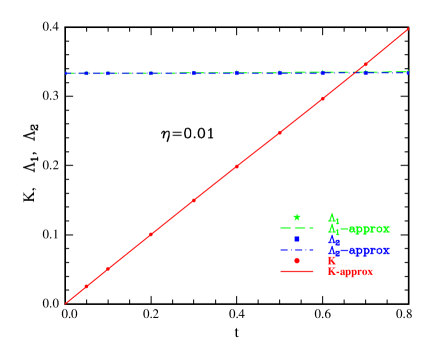
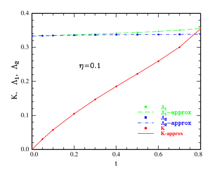
Figure 2: (Color online) Comparison between exact numerical and approximate analytical results for the parameters $K$, $\Lambda_{1},$ and $\Lambda_{2}$ as a function of $t$, for anisotropy degree $\alpha=1/2$ and two values of the packing fraction: $\eta=0.01$ (top panel) and $\eta=0.1$ (bottom panel).

In order to assess the precision of previous approximations, we have calculated $K$, $\Lambda_{1}$ and $\Lambda_{2}$ by two methods: i) solving numerically Eqs. (126), and ii) using our analytic approximations. After fixing $\alpha=1/2,$ we have increased the adhesion strength (or decreased the temperature) from $t=0$ (HS limit) up to $t=0.8$, for some representative values of the volume fraction ($\eta=0.01$, $0.1$, $0.2$ and $0.4)$. The maximum value of $t$ corresponds to $\tau=1/(12t)\simeq 0.1$, which lies close to the critical temperature of the isotropic SHS fluid. On the other hand, $\eta=0.01$ has been chosen to illustrate the fact that, as $\eta\rightarrow 0$, the parameter $K$ tends to $\alpha t$. The linear dependence of $K$ on $t$ in this case is clearly visible in the top panel of Figure 2.

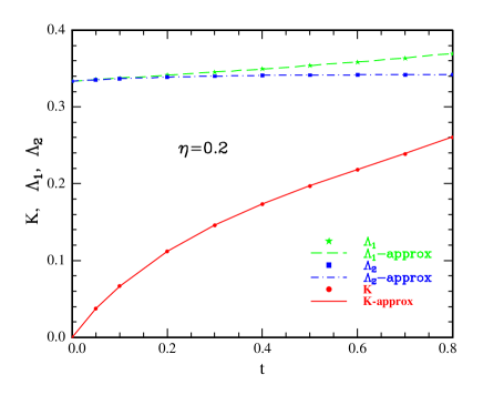
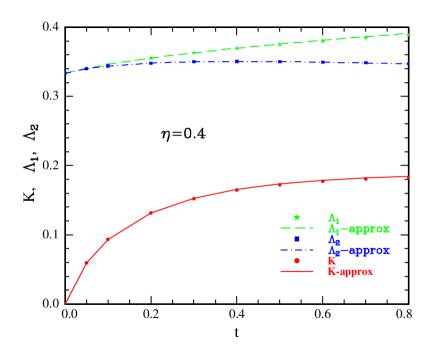
Figure 3: (Color online) Same as in Figure 2, but for $\eta=0.2$ (top panel) and $\eta=0.4$ (bottom panel).

In Figures 2 and 3 the exact and approximate results for $K$, $\Lambda_{1}$ and $\Lambda_{2}$ are compared. The agreement is excellent: at $\eta=0.1$, $0.2$ and $0.4$, the relative error on $K$ does not exceed $0.1\%$, $0.4\%$ and $1\%$, respectively, while the maximum of the absolute relative errors on $\Lambda_{1}$ and $\Lambda_{2}$ always remain less than $0.05$, $0.2$ and $0.6~{}\%$ in the three above-mentioned cases. It is worth noting that, as $\eta$ increases, the variations of $\Lambda_{1}$ and $\Lambda_{2}$ are always relatively small; on the contrary, $K$ experiences a marked change, with a progressive lowering of the relevant curve.

VI Some illustrative results on the local orientational structure

Armed with the knowledge of the analytic expression for the $q_{m}s$ a rapid numerical calculation of the three harmonic coefficients $\left\{h_{0},h_{\Delta},h_{D}\right\}$ appearing in

$$g^{\mathrm{PY-OL}}(1,2)=1+h_{0}(r)+h_{\Delta}(r)\Delta(1,2)+h_{D}(r)D(1,2).$$ (91)

can be easily obtained as follows. From the second Baxter IE (60), one can generate $h(r)$ directly from $q(r)$, avoiding the passage through $c(r)$. From $\left\{q_{0},q_{1},q_{2}\right\}$ one first obtains $\left\{h_{0},h_{1},h_{2}\right\}$, by applying a slight extension of Perram’s numerical method Perram75 and then derive $\left\{h_{0},h_{\Delta},h_{D}\right\}$, according to the above-mentioned recipes.

The main aim of the present paper was to present the necessary mathematical machinery to investigate thermophysical properties. We now illustrate the interest of the model by reporting some preliminary numerical results on the orientational dependence of $g^{\mathrm{PY-OL}}(1,2)$ – i.e. on the local orientational structure – as a consequence of the anisotropic adhesion. A more detailed analysis will be reported in a forthcoming paper.

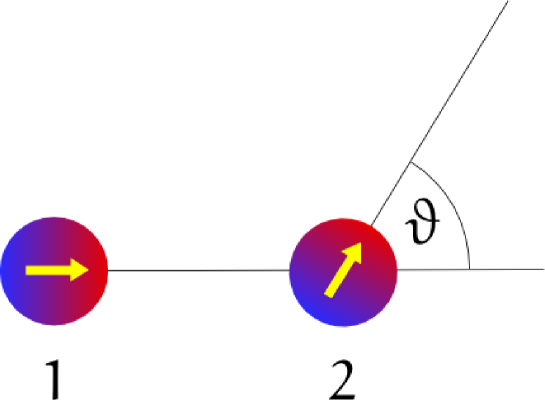
Figure 4: (Color online) Illustration of the simple configuration discussed in the text and chosen to define some radial sections through the multidimensional plot of $g(1,2)$.

Consider the configuration depicted in Figure 4. Let a generic particle $1$ be fixed at a position $\mathbf{r}_{1\text{ }}$in the fluid with orientation $\mathbf{u}_{1\text{ }}$, and consider another particle $2$ located along the straigth half-line which originates from the center of $1$ and with direction $\mathbf{u}_{1\text{ }}$. This second particle has then a fixed distance $r$ from $1$, but can assume all possible orientations $\mathbf{u}_{2\text{ }}$, which – by axial symmetry – can be described by a single polar angle $\theta\equiv\theta_{2}$ (i.e., the angle between $\mathbf{u}_{1\text{ }}$and $\mathbf{u}_{2\text{ }}$) with respect to the intermolecular reference frame. Within this geometry, we have $\left(\theta_{1},\varphi_{1}\right)=(0,0)$ and $\varphi_{2}=0$, obtaining $\Delta(1,2)=\cos\theta$, $D(1,2)=2\cos\theta$. Consequently, $g(1,2)=g(r,\theta_{1},\varphi_{1},\theta_{2},\varphi_{2})$ reduces to

$$g(r,\theta)=g_{0}(r)+\left[h_{\Delta}(r)+2h_{D}(r)\right]\cos\theta,$$ (92)

where $\theta\equiv\theta_{2}$, and $g_{0}(r)=1+h_{0}(r)$ is the radial distribution function of the reference isotropic SHS fluid.

Clearly, $g(r,\theta)$ is proportional to the probability of finding, at a distance $r$ from a given molecule $1$, a molecule $2$ having a relative orientation $\theta$. We consider the three most significant values of this angle: i) $\theta=0$, which corresponds to the ‘parallel’ configuration of $\mathbf{u}_{1}$ and $\mathbf{u}_{2}$; ii) $\theta=\pi/2$, for the ‘orthogonal’ configuration; and $\theta=\pi$, for the two ‘antiparallel’ (head-to-head and tail-to-tail) configurations. From Eq. (92) it follows that

$$\begin{array}[]{c}g^{\mathrm{par}}(r)=g(r,0)=g_{0}(r)+\left[h_{\Delta}(r)+2h_{D}(r)\right],\text{ \ \ \ }\\ g^{\mathrm{ortho}}(r)=g(r,\pi/2)=g_{0}(r),\text{ \ \ \ \ \ \ \ \ \ \ \ \ \ \ \ \ \ \ \ \ \ \ \ \ }\\ g^{\mathrm{antipar}}(r)=g(r,\pi)=g_{0}(r)-\left[h_{\Delta}(r)+2h_{D}(r)\right].\text{ \ }\end{array}$$ (93)

Note that $g^{\mathrm{ortho}}(r)$ coincides with the isotropic result $g_{0}(r)$.

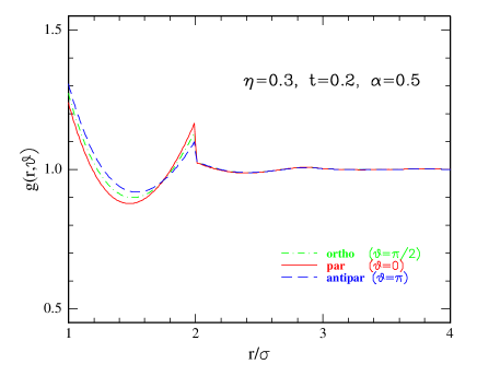
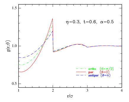
Figure 5: (Color online) Sections through $g(1,2)$, with particles 1 and 2 in the configuration shown by the previous Figure, calculated as a function of $r$ for fixed relative orientations: $\theta=0$ (parallel configuration), $\theta=\pi/2$ (orthogonal configuration), and $\theta=\pi$ (antiparallel configurations).

In Figures 5 we depict the above sections through the three-dimensional surface corresponding to $g(r,\theta)$, i.e., $g^{\mathrm{par}}(r)$, $g^{\mathrm{ortho}}(r)$ and $g^{\mathrm{antipar}}(r)$, for $\eta=0.3$ with $t=0.2$ and $t=0.6$, respectively, at the highest asymmetry value admissible in the present model, i.e. $\alpha=1/2$. The most significant features from these plots are: i) $g^{\mathrm{antipar}}(\sigma^{+})>g^{\mathrm{par}}(\sigma^{+})$; ii) for $r>2\sigma$ $g^{\mathrm{antipar}}(r)\approx g^{\mathrm{par}}(r)\approx g_{0}(r)$, i.e., the anisotropic adhesion seems to affect only the first coordination layer, $\sigma<r<2\sigma$, around each particle.

The interpretation of these results is the following. In view of i) we see that the parallel configuration is less probable than the antiparallel one at contact. Such a finding, together with ii), means that chain formation characteristic of polymerization is inhibited by the short-ranged anisotropic adhesion exploited here. This strictly contrasts with the case of long-ranged DHS fluids, where it is believed Camp00 ; Tlusty00 that chaining phenomena might preempt the gas-liquid transition. This specific feature of the present model is extremely interesting and we plan a throughout investigation on this topic in a future publication.

VII Phase stability

In view of previous findings, a very natural question is whether the addition of our anisotropic sticky term to the potential changes phase stability and phase transition curves with respect to the corresponding isotropic case. We believe the answer to be positive. This is strongly suggested by results obtained for similar anisotropic models, such as hard spheres with ‘sticky points’ Sciortino05 ; Bianchi06 ; Michele06 ; Lomakin99 ; Starr03 ; Zhang04 ; Glotzer04a ; Glotzer04b ; Sciortino07 or ‘sticky patches’ Jackson88 ; Ghonasgi95 ; Sear99 ; Mileva00 ; Kern03 ; Zhang05 ; Fantoni07 .

We now briefly comment on this issue. Within our formalism, this problem of stability can be conveniently analyzed using standard formalism devised to this aim Gray84 ; Stecki81 ; Chen92 ; Klapp97 .

We start from the stability condition with respect to small but arbitrary fluctuations of the one-particle density $\rho(1)$ from the equilibrium configuration, denoted as ’eq’ Stecki81 ; Chen92 ; Klapp97 ,

$$\int d(1)\int d(2)\left[\frac{\delta(1,2)}{\rho(1)}-c\left(1,2\right)\right]_{eq}\delta\rho(1)\delta\rho(2)>0.$$ (94)

Here $d(i)$ stands for $d\mathbf{r}_{i}~{}d\Omega_{i}$, $i=1,2$, and we assume the equilibrium one-particle density to be $\rho/4\pi$ Stecki81 ; Chen92 ; Klapp97 .

We expand the fluctuations both in Fourier modes and in spherical harmonics Gray84

$$\delta\rho\left(j\right)\equiv\delta\rho\left(\mathbf{r}_{j},\Omega_{j}\right) = \int\frac{d\mathbf{k}}{\left(2\pi\right)^{3}}~{}\mathrm{e}^{\mathrm{i}\mathbf{k}\cdot\mathbf{r}_{j}}\sum_{l=0}^{+\infty}\sum_{m=-l}^{+l}\delta\tilde{\rho}\left(\mathbf{k}\right)Y_{lm}\left(\Omega_{j}\right).$$ (95)

Using the orthogonality relation Gray84

$$\int d\Omega~{}Y_{lm}^{*}\left(\Omega\right)Y_{l^{\prime}m^{\prime}}\left(\Omega\right) = \delta_{ll^{\prime}}\delta_{mm^{\prime}},$$ (96)

standard manipulations Klapp97 show that condition (94) can be recast into the form

$$\sum_{l_{1},l_{2}=0}^{+\infty}\sum_{m_{1}=-l_{1}}^{+l_{1}}\sum_{m_{2}=-l_{2}}^{+l_{2}}\int\frac{d\mathbf{k}}{\left(2\pi\right)^{3}}~{}\delta\tilde{\rho}_{l_{1}m_{1}}\left(\mathbf{k}\right)\delta\tilde{\rho}_{l_{1}m_{1}}^{*}\left(\mathbf{k}\right)\tilde{A}_{l_{1}m_{1}l_{2}m_{2}}\left(\mathbf{k}\right) >0$$ , (97)

where the matrix elements $\tilde{A}_{l_{1}m_{1}l_{2}m_{2}}\left(\mathbf{k}\right)$ are given by

$$\tilde{A}_{l_{1}m_{1}l_{2}m_{2}}\left(\mathbf{k}\right) = \left(-1\right)^{m_{1}}\frac{4\pi}{\rho}\delta_{l_{1}l_{2}}\delta_{m_{1},-m_{2}}-\int d\Omega_{1}\int d~{}\Omega_{2}Y_{l_{1}m_{1}}\left(\Omega_{1}\right)Y_{l_{2}m_{2}}\left(\Omega_{2}\right)$$

$$\times \int d\mathbf{r}~{}\mathrm{e}^{\mathrm{i}\mathbf{k}\cdot\mathbf{r}}c\left(\mathbf{r},\Omega_{1},\Omega_{2}\right).$$

The problem of the stability has been reported to the character of the eigenvalues of matrix (VII). This turns out to be particularly simple in our case. Using the results (108) it is easy to see that

$$\int d\mathbf{r}~{}\mathrm{e}^{\mathrm{i}\mathbf{k}\cdot\mathbf{r}}c\left(\mathbf{r},\Omega_{1},\Omega_{2}\right) = \tilde{c}_{0}\left(k\right)+\tilde{c}_{\Delta}\left(k\right)\Delta\left(\Omega_{1},\Omega_{2}\right)+\overline{c}_{D}\left(k\right)D\left(\Omega_{1},\Omega_{2},\Omega_{k}\right).$$ (99)

Insertion of Eq.(99) into Eq.(VII) leads to

$$\tilde{A}_{l_{1}m_{1}l_{2}m_{2}}\left(\mathbf{k}\right) = \left(-1\right)^{m_{1}}\frac{4\pi}{\rho}\delta_{l_{1}l_{2}}\delta_{m_{1},-m_{2}}$$

$$- \left[\tilde{c}_{0}\left(k\right)I_{l_{1}m_{1}l_{2}m_{2}}^{(0)}+\tilde{c}_{\Delta}\left(k\right)I_{l_{1}m_{1}l_{2}m_{2}}^{(\Delta)}+\tilde{c}_{D}\left(k\right)I_{l_{1}m_{1}l_{2}m_{2}}^{(D)}\right],$$

where we have introduced the following integrals, which can be evaluated in the intermolecular frame, using standard properties of the spherical harmonics Gray84

$$I_{l_{1}m_{1}l_{2}m_{2}}^{(0)} \equiv \int d\Omega_{1}\int d\Omega_{2}~{}Y_{l_{1}m_{1}}\left(\Omega_{1}\right)Y_{l_{2}m_{2}}\left(\Omega_{2}\right)=4\pi\delta_{l_{1}0,}\delta_{l_{2},0}\delta_{m_{1}0}\delta_{m_{2}}\delta_{0}$$ (101)

$$I_{l_{1}m_{1}l_{2}m_{2}}^{(\Delta)} \equiv \int d\Omega_{1}\int d\Omega_{2}~{}Y_{l_{1}m_{1}}\left(\Omega_{1}\right)Y_{l_{2}m_{2}}\left(\Omega_{2}\right)~{}\Delta\left(\Omega_{1},\Omega_{2}\right)=\frac{4}{3}\pi\delta_{l_{1}1}\delta_{l_{2},1}\delta_{m_{1}0}\delta_{m_{2},0}$$

$$I_{l_{1}m_{1}l_{2}m_{2}}^{(D)}\left(\cos\theta\right) \equiv \int d\Omega_{1}\int d\Omega_{2}~{}Y_{l_{1}m_{1}}\left(\Omega_{1}\right)Y_{l_{2}m_{2}}\left(\Omega_{2}\right)D\left(\Omega_{1},\Omega_{2},\Omega_{k}\right)$$

$$= \frac{4}{3}\pi\delta_{l_{1},1}\delta_{l_{2},1}\delta_{m_{1},0}\delta_{m_{2},0}~{}2~{}P_{2}\left(\cos\theta\right)$$

and where $P_{2}(x)=(3x^{2}-1)/2$ is the second Legendre polynomial.

Hence, the matrix (VII) is diagonal and the relevant terms are

$$\tilde{A}_{0000}\left(k\right) = 4\pi\left[\frac{1}{\rho}-\tilde{c}_{0}\left(k\right)\right],$$ (102)

whose positiveness is recognized as the isotropic stability condition, and

$$\tilde{A}_{1010}\left(\mathbf{k}\right) = 4\pi\left\{\frac{1}{\rho}-\frac{1}{3}\left[\tilde{c}_{\Delta}\left(k\right)+2P_{2}\left(\cos\theta\right)\overline{c}_{D}\left(k\right)\right]\right\}.$$ (103)

All remaining diagonal terms have the form $\tilde{A}_{l0l0}=4\pi/\rho>0$.

In order to test for possible angular instabilities, we consider the limit $k\to 0$ of Eq. (103) namely

$$\tilde{A}_{1010}\left(0\right) = \frac{4\pi}{\rho}\left\{1-\frac{\rho}{3}\left[\tilde{c}_{\Delta}\left(0\right)+2P_{2}\left(\cos\theta\right)\overline{c}_{D}\left(0\right)\right]\right\}.$$ (104)

This can be quickly computed with the aid of Eqs. (46), (59), the fact that $\bar{c}_{D}(0)=\tilde{c}_{D}^{0}(0)$ and the identity (70). We find

$$\tilde{A}_{1010}\left(0\right) = \frac{4\pi}{\rho}a_{1}^{2},$$ (105)

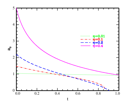
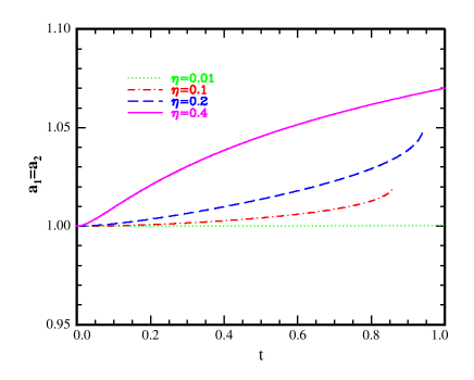
Figure 6: (Color online) Evaluation of quantities $a_{0}$ (top panel) and $a_{1}=a_{2}$ (bottom panel) as a function of $t$ for various packing fractions ranging from $\eta=0.01$ to $\eta=0.4$. These are computed from Eq.(64) with $m=0,1$. Note that for both $\eta=0.1$ and $\eta=0.2$, $a_{0}=0$ corresponds to the onset of isotropic instability.

which is independent of the angle $\theta$. This value is found to be always positive as $a_{1}>0$ (see Fig.6). Within this first-order approximation, therefore the only instability in the system stems from the isotropic compressibility. The reason for this can be clearly traced back to the first-order approximation to the angular dependence of the correlation functions. If quadratic terms in $\Delta$ and $D$ were included into the series expansion for correlation functions, the particular combination leading to a cancellation of the angular dependence in the stability matrix $\tilde{A}_{l_{1}m_{1}l_{2}m_{2}}\left(0\right)$ would not occur, leading to a different result.

This fact is consistent with the more general statement that, in any approximate theory, thermodynamics usually requires a higher degree of theoretical accuracy than the one sufficient for obtaining significant structural data. Conceptually, the need of distinguishing structural results from thermodynamical ones is rather common. For instance, in statistical mechanics of liquids it is known that approximating the model potential only with its repulsive part (for instance, the hard sphere term) can account for all essential features of the structure, but yields unsatisfactory thermodynamics. On the other hand, the present paper refers to a simplified statistical-mechanical tool, i.e. the OZ equation within our PY-OL closure, which has been explicitly selected to allow an analytical solution. Our results however indicate that the first-order expansion used in the PY-OL closure can give reasonable information about structure, but not on thermodynamics, where a higher level of sophistication is required.

VIII Concluding remarks

In this paper we have discussed an anisotropic variation of the original Baxter model of hard spheres with surface adhesion. In addition to the HS potential, molecules of the fluid interact via an isotropic sticky attraction plus an additional anisotropic sticky correction, whose strength depends on the orientations of the particles in dipolar way. By varying the value of a parameter $\alpha$, the anisotropy degree can be changed. Consequenly, the strength of the total sticky potential can vary from twice the isotropic one down to the limit of no adhesion (HS limit). These particles may be regarded as having two non-uniform, hemispherical, ‘dipolar-like patches’, thus providing a link with uniformly adhesive patches Jackson88 ; Ghonasgi95 ; Sear99 ; Mileva00 ; Kern03 ; Zhang05 ; Fantoni07 .

We have obtained a full analytic solution of the molecular OZ equation, within the PY-OL approximation, by using Wertheim’s technique Wertheim71 . Our PY-OL approximation should be tested against exact computer simulations, in order to assess its reliability. Nevertheless, we may reasonably expect the results to be reliable even at experimentally significant densities, notwithstanding the truncation of the higher-orders terms in the angular expansion. Only one equation, for the parameter $K$, has to be solved numerically. In additon, we have provided analytic approximations to $K$, $\Lambda_{1}$ and $\Lambda_{2}$ so accurate that, in practice, the whole solution can really be regarded as fully analytical. From this point of view, the present paper complements the above-mentioned previous work by Blum et al. Blum90 .

We have also seen that thermophysical properties require a more detailed treatment of the angular part than the PY-OL closure. Nonetheless, even within the PY-OL oversimplified framework, our findings are suggestive of a dependence of the fluid-fluid coexistence line on anisotropy.

Our analysis envisions a number of interesting perspectives, already hinted by the preliminary numerical results reported here. It would be very interesting to compare the structural and thermodynamical properties of this model with those stemming from truly dipolar hard spheres Stecki81 ; Chen92 ; Klapp97 . The possibility of local orientational ordering can be assessed by computing the pair correlation function $g(1,2)$ for the most significant interparticle orientations. We have shown that this task can be easily performed within our scheme. This should provide important information about possible chain formation and its subtle interplay with the location of the fluid-fluid transition line. The latter bears a particular interest in view of the fact that computer simulations on DHS are notoriously difficult and their predictions regarding the location of such a transition line have proven so far unconclusive Frenkel02 . The long-range nature of DHS interactions may in fact promote polymerization preempting the usual liquid-gas transition Tlusty00 . Our preliminary results on the present model strongly suggest that this is not the case for sufficiently short-ranged interactions, thus allowing the location of such a transition line to be studied as a function of the anisotropy degree of the model. Our sticky interactions have only attractive adhesion, the only repulsive part being that pertinent to hard spheres, whereas the DHS potential is both attractive and repulsive, depending on the orientations.

Finally, information about the structural ordering in the present model would neatly complement those obtained by us in a recent parallel study on a SHS fluid with one or two uniform circular patches Fantoni07 . Work along this line is in progress and will be reported elsewhere.

Appendix A Extension of Wertheim’s approach

The Fourier transform of the excess PY-OL equation, Eq. (17), reads

$$\widehat{h}_{\mathrm{ex}}(\mathbf{k},\Omega_{1},\Omega_{2})=\widehat{c}_{\mathrm{ex}}(\mathbf{k},\Omega_{1},\Omega_{2})+\rho\ \left\langle\ \widehat{c}_{\mathrm{ex}}(\mathbf{k},\Omega_{1},\Omega_{3})\ \widehat{h}_{\mathrm{ex}}(\mathbf{k},\Omega_{3},\Omega_{2})\ \right\rangle_{\Omega_{3}}$$ (106)

(the superscripts have been omitted for simplicity). In order to evaluate the angular average, we first need the FT of $c$ and $h$. The FT integral (8) may be rewritten as

$$\int_{0}^{\infty}dr\ r^{2}\int d\Omega_{r}\ \exp(i\mathbf{k\cdot r})\ \left[\cdots\right]=\int_{0}^{\infty}dr\ r^{2}\int_{0}^{2\pi}d\phi\int_{-1}^{+1}d\left(\cos\theta\right)\ e^{ikr\cos\theta}\ \left[\cdots\right].$$

Let us now apply this operator to $F_{\mathrm{ex}}(1,2)$ ($F=c,h$), expressed as

$$F_{\mathrm{ex}}(\mathbf{r},\Omega_{1},\Omega_{2})=F_{\Delta}(r)\ \Delta(\Omega_{1},\Omega_{2})+F_{D}(r)\ D(\Omega_{1},\Omega_{2},\Omega_{r}),$$ (107)

and first perform the angular integration $\int d\Omega_{r}$, recalling that Wertheim71

$$\begin{array}[]{c}\int d\Omega_{r}~{}\exp(i\mathbf{k\cdot r})\ \ 1=4\pi\ j_{0}(kr)\ 1\text{ \ \ \ }\\ \int d\Omega_{r}\ \exp(i\mathbf{k\cdot r})\ \ \Delta(\Omega_{1},\Omega_{2})=4\pi\ j_{0}(kr)\ \Delta(\Omega_{1},\Omega_{2})\text{\ \ \ \ }\\ \int d\Omega_{r}\ \exp(i\mathbf{k\cdot r})\ \ D(\Omega_{1},\Omega_{2},\Omega_{r})=-4\pi\ j_{2}(kr)\ D(\Omega_{1},\Omega_{2},\Omega_{k}),\\ \end{array}$$ (108)

where $j_{0}(x)=x^{-1}\sin x$ and $j_{2}(x)=3x^{-3}\sin x-3x^{-2}\cos x-j_{0}(x)$ are Bessel functions, and

$$D(\Omega_{1},\Omega_{2},\Omega_{k})=3(\mathbf{u}_{1}\cdot\hat{\mathbf{k}})(\mathbf{u}_{2}\cdot\hat{\mathbf{k}})-\mathbf{u}_{1}\cdot\mathbf{u}_{2}\equiv D_{k}(1,2),$$

with $\hat{\mathbf{k}}=\mathbf{k}/k$. We get

$$\widehat{F}_{\mathrm{ex}}(\mathbf{k},\Omega_{1},\Omega_{2})=\widetilde{F}_{\Delta}(k)\ \Delta(\Omega_{1},\Omega_{2})+\overline{F}_{D}(k)\ D(\Omega_{1},\Omega_{2},\Omega_{k}),$$

where $\widetilde{F}_{\Delta}(k)$ is the usual FT of the spherically symmetric function $F_{\Delta}(r)$: $\ \widetilde{F}_{\ldots}(k)=4\pi\int_{0}^{\infty}dx\ x^{2}\ j_{0}(kx)F_{\ldots}(x)$. On the other hand, $\overline{F}_{D}(k)=-4\pi\int_{0}^{\infty}dx\ x^{2}\ j_{2}(kx)F_{D}(x)$, which is the Hankel transform of $F_{D}(r)$, may conveniently be considered as the FT of a ‘modified’ function $F_{D}^{0}(r)$, i.e. $\overline{F}_{D}(k)=\widetilde{F}_{D}^{0}(k)$. Taking the inverse FT of $\overline{F}_{D}(k)$ yields

$$F_{D}^{0}(r)=\frac{1}{2\pi^{2}}\int_{0}^{\infty}dk\ k^{2}\ j_{0}(kr)\overline{F}_{D}(k)=F_{D}(r)-3\int_{r}^{\infty}\frac{F_{D}(x)}{x}\ dx,$$ (109)

with the help of the identity

$$\int_{0}^{\infty}dk\ k^{2}\ j_{0}(kr)\ j_{2}(kx)=\frac{\pi}{2}\left[\frac{3\theta\left(x-r\right)}{x^{3}}-\frac{\delta\left(x-r\right)}{x^{2}}\right].$$

In conclusion, the FT of $F_{\mathrm{ex}}(1,2)$ reads

$$\widehat{F}_{\mathrm{ex}}(\mathbf{k},\Omega_{1},\Omega_{2})=\widetilde{F}_{\Delta}(k)\ \Delta(\Omega_{1},\Omega_{2})+\widetilde{F}_{D}^{0}(k)\ D(\Omega_{1},\Omega_{2},\Omega_{k}),$$ (110)

with $F$ standing for $h$ or $c$.

Let us now define the angular convolution of two functions as

$$A\circ B=B\circ A\equiv\left\langle A(\Omega_{1},\Omega_{3})\ B(\Omega_{3},\Omega_{2})\right\rangle_{\Omega_{3}}.\$$

Wertheim Wertheim71 demonstrated that the rotational invariants $1,$ $\Delta,$ and $D$ form a closed group under angular convolution; that is, the angular convolution of any two members of this set yields only a function in the same set, or zero, according to the following multiplication table

$\circ$		$1$		$\Delta$		$D_{k}$
$1$		$1$		$0$		$0$
$\Delta$		$0$		$\Delta/3$		$D_{k}/3$
$D_{k}$		$0$		$D_{k}/3$		$(D_{k}+2\Delta)/3$

Table 1: Angular convolutions of the basis functions $1,\Delta$ and $D_{k}$.

Substituting the expressions for $\widehat{c}_{\mathrm{ex}}$ and$\ \widehat{h}_{\mathrm{ex}}$ given by Eq. (110) into the angular average $\widehat{c}_{\mathrm{ex}}\circ\widehat{h}_{\mathrm{ex}}=\left\langle\widehat{c}_{\mathrm{ex}}(\mathbf{k},\Omega_{3},\Omega_{2})\ \widehat{h}_{\mathrm{ex}}(\mathbf{k},\Omega_{3},\Omega_{2})\right\rangle_{\Omega_{3}}$, with the help of Table I we obtain

$$\widehat{c}_{\mathrm{ex}}\circ\widehat{h}_{\mathrm{ex}} = \widetilde{c}_{\Delta}\widetilde{h}_{\Delta}\frac{1}{3}\Delta+\widetilde{c}_{\Delta}\widetilde{h}_{D}^{0}\frac{1}{3}D_{k}$$

$$+\widetilde{c}_{D}^{0}\widetilde{h}_{\Delta}\frac{1}{3}D_{k}+\widetilde{c}_{D}^{0}\widetilde{h}_{D}^{0}\frac{1}{3}\left(2\Delta+D_{k}\right).$$

Inserting this result into Eq. (106) and equating the coefficients of $\Delta,$ and $D$ separately, one finds that the $\mathbf{k}$-space excess PY-OL equation splits into two coupled integral equations, i.e.,

$$\left\{\begin{array}[]{c}\widetilde{h}_{\Delta}-\widetilde{c}_{\Delta}=\frac{1}{3}\rho~{}\left(\ \widetilde{c}_{\Delta}\widetilde{h}_{\Delta}+2\ \widetilde{c}_{D}^{0}\widetilde{h}_{D}^{0}\ \right)\text{\ \ \ \ \ \ \ \ \ \ \ \ \ }\\ \widetilde{h}_{D}^{0}-\widetilde{c}_{D}^{0}=\frac{1}{3}\rho~{}\left(\ \widetilde{c}_{\Delta}\widetilde{h}_{D}^{0}+\widetilde{c}_{D}^{0}\widetilde{h}_{\Delta}+\widetilde{c}_{D}^{0}\widetilde{h}_{D}^{0}\ \right).\text{ \ \ }\end{array}\right.$$

Coming back to the $\mathbf{r}$-space, one gets the following equations

$$\left\{\begin{array}[]{c}h_{\Delta}(r)=c_{\Delta}(r)+\frac{1}{3}\rho~{}\left(\ c_{\Delta}\star h_{\Delta}+2\ c_{D}^{0}\star h_{D}^{0}\ \right)\text{\ \ \ \ \ \ \ \ \ \ \ }\\ h_{D}^{0}(r)=c_{D}^{0}(r)+\frac{1}{3}\rho~{}\left(\ c_{\Delta}\star h_{D}^{0}+c_{D}^{0}\star h_{\Delta}+c_{D}^{0}\star h_{D}^{0}\ \right).\end{array}\right.$$ (111)

In particular, since $h_{D}(r)=0$ for  $0<r<\sigma$, Eq. (33) yields $h_{D}^{0}(r)=-3K$ for  $0<r<\sigma$, with $K$ being a dimensionless parameter defined by

$$K=\int_{\sigma^{-}}^{\infty}\frac{h_{D}(x)}{x}\ dx.$$ (112)

The exact core conditions for Eqs. (111) are

$$\left.\begin{array}[]{c}\text{ \ }h_{\Delta}(r)=0\text{ \ \ \ \ \ \ }\\ h_{D}^{0}(r)=-3K\end{array}\right\}\text{ \ \ \ \ \ for \ }0<r<\sigma.$$ (113)

Now, in the PY-OL closure for the DCFs, Eqs. (24), the closure for $c_{D}(r)$ must be replaced with that corresponding to $c_{D}^{0}(r)$ (for simplicity, here and in the following we omit the superscript PY-OL). In order to derive this, let us start from $c_{D}(r)=c_{D\text{,reg}}(r)+\Lambda_{D}\ \sigma\delta\left(r-\sigma\right),$ where $c_{D\text{,reg}}(r)=f^{\mathrm{HS}}(r)\ y_{D}^{\mathrm{PY}}(r)=0$ for $r\geq\sigma$. Then Eq. (33) yields

$$c_{D}^{0}(r)=c_{D}(r)-3\int_{r}^{\sigma}\frac{c_{D\text{,reg}}(x)}{x}\ dx-3\Lambda_{D}\ \theta(\sigma-r),$$

since $\int_{r}^{\infty}\delta\left(x-\sigma\right)\ x^{-1}\ dx=\sigma^{-1}\theta(\sigma-r)$ note1 . So we get

$$c_{D}^{0}(r)=c_{D}(r)\text{ \ \ \ for \ }r\geq\sigma,$$ (114)

and the required new closures are

$$\left.\begin{array}[]{c}c_{\Delta}(r)=\Lambda_{\Delta}\ \sigma\delta\left(r-\sigma\right)\\ c_{D}^{0}(r)=\Lambda_{D}\ \sigma\delta\left(r-\sigma\right)\end{array}\right\}\text{ \ \ \ \ \ }r\geq\sigma.$$ (115)

In order to decouple the two integral equations for $\Delta$- and $D$-coefficients, we then introduce two new unknown functions, which are linear combinations of the previous ones. Defining

$$\ \widetilde{F}_{\mathrm{new}}=\lambda_{1}\widetilde{F}_{\Delta}+\lambda_{2}\widetilde{F}_{D}^{0}\text{ \ \ \ \ \ \ }\left(F=c,h\right)$$

and using Eqs. (A) leads to

$$\widetilde{h}_{\mathrm{new}}-\widetilde{c}_{\mathrm{new}} = \lambda_{1}\left(\widetilde{h}_{\Delta}-\widetilde{c}_{\Delta}\right)+\lambda_{2}\left(\widetilde{h}_{D}^{0}-\widetilde{c}_{D}^{0}\right)$$

$$= \frac{1}{3}\rho~{}\left[\ \lambda_{1}\widetilde{c}_{\Delta}\widetilde{h}_{\Delta}+\lambda_{2}\left(\widetilde{c}_{\Delta}\widetilde{h}_{D}^{0}+\widetilde{c}_{D}^{0}\widetilde{h}_{\Delta}\right)+\left(2\lambda_{1}+\lambda_{2}\right)\widetilde{c}_{D}^{0}\widetilde{h}_{D}^{0}\right].$$

Requiring the second member of this equation to be proportional to $\rho\widetilde{c}_{\mathrm{new}}\widetilde{h}_{\mathrm{new}}$ – that is, equal to $\mathcal{L}\rho\left(\lambda_{1}\widetilde{c}_{\Delta}+\lambda_{2}\widetilde{c}_{D}^{0}\right)\left(\lambda_{1}\widetilde{h}_{\Delta}+\lambda_{2}\widetilde{h}_{D}^{0}\right)$, with $\mathcal{L}$ being the proportionality constant –, yields the following conditions

$$\left\{\begin{array}[]{c}\frac{1}{3}\lambda_{1}=\mathcal{L}\lambda_{1}^{2}\text{\ \ \ \ \ \ \ \ \ \ \ \ \ \ \ \ \ \ \ \ \ \ \ \ \ \ \ \ }\\ \frac{1}{3}\lambda_{2}=\mathcal{L}\lambda_{1}\lambda_{2}\text{ \ \ \ \ \ \ \ \ \ \ \ \ \ \ \ \ \ \ \ \ \ \ \ }\\ \frac{1}{3}\left(2\lambda_{1}+\lambda_{2}\right)=\mathcal{L}\lambda_{2}^{2}\ \ \text{\ }.\text{ \ \ \ \ \ \ \ \ \ \ \ }\end{array}\right.$$

An infinite number of solutions are possible, and correspond to

$$\left(\lambda_{1},\lambda_{2}\right)=\frac{1}{3\mathcal{L}_{1}}\left(1,-1\right)\text{, \ \ \ \ \ \ \ \ \ \ and \ \ \ \ \ }\left(\lambda_{1},\lambda_{2}\right)=\frac{1}{3\mathcal{L}_{2}}\left(1,2\right),$$

since there is no need for the proportionality constant to have the same value in the two cases, i.e. $\xi_{2}$ can differ from $\xi_{1}$. As a consequence, we can write the two new $h_{\mathrm{new}}(r)$ as

$$\left\{\begin{array}[]{c}h_{1}\left(r\right)=\left(3\mathcal{L}_{1}\right)^{-1}\left[h_{\Delta}(r)-h_{D}^{0}(r)\right]\text{ \ }\\ h_{2}\left(r\right)=\left(3\mathcal{L}_{2}\right)^{-1}\left[h_{\Delta}(r)+2h_{D}^{0}(r)\right],\end{array}\right.$$ (116)

while similar expressions hold for $c_{1}$ and $c_{2}$. From Eqs. (113) it follows that: $\ h_{1}(r)=K/\mathcal{L}_{1}$  and $h_{2}(r)=-2K/\mathcal{L}_{2}$   for  $0<r<\sigma.$

In Ref. I Wertheim chose $\mathcal{L}_{1}=-K$ and $\mathcal{L}_{2}=2K$ Wertheim71 , which leads to

$$\left\{\begin{array}[]{c}F_{1}\left(r\right)=\frac{1}{3K}\left[F_{D}^{0}(r)-F_{\Delta}(r)\right]\text{ }\\ F_{2}\left(r\right)=\frac{1}{3K}\left[F_{D}^{0}(r)+\frac{1}{2}F_{\Delta}(r)\right]\end{array}\right.\text{\ \ \ \ }\left(F=c,h\right),$$ (117)

$$\left\{\begin{array}[]{c}\rho_{1}=-K\rho\text{ }\\ \rho_{2}=2K\rho,\end{array}\right.\qquad\qquad\left\{\begin{array}[]{c}h_{1}(r)=-1\\ h_{2}(r)=-1\end{array}\right.\text{ \ \ \ \ \ for \ }0<r<\sigma$$ (118)

(in Ref. I, $F_{1}$ and $F_{2}$ were denoted as $F_{-}$ and $F_{+}$, respectively). Clearly, Wertheim’s choice has the advantage of providing, for all the three ‘hypothetical’ fluids, core conditions of the typical HS form: $h_{m}(r)=-1$ for  $0<r<\sigma$ ($m=0,1,2$). The cost to pay is the introduction of ‘modified densities’ for the ‘auxiliary’ fluids $1$ and $2$ (the negative sign of $\rho_{1}$ poses no special difficulty).

On the other hand, it is would be equally proposable the choice $\mathcal{L}_{1}=\mathcal{L}_{2}=1$, which leads to

$$\left\{\begin{array}[]{c}F_{1}\left(r\right)=\frac{1}{3}\ \left[F_{\Delta}(r)-F_{D}^{0}(r)\right]\text{ \ \ }\\ F_{2}\left(r\right)=\frac{1}{3}\ \left[F_{\Delta}(r)+2F_{D}^{0}(r)\right]\text{ }\end{array}\right.\text{\ \ \ \ }\left(F=c,h\right),$$

$$\left\{\begin{array}[]{c}\rho_{1}=\rho\text{ }\\ \rho_{2}=\rho,\end{array}\right.\qquad\qquad\left\{\begin{array}[]{c}h_{1}(r)=K\text{ \ \ }\\ h_{2}(r)=-2K\end{array}\right.\text{ \ \ \ \ \ for \ }0<r<\sigma.$$

The advantage of this second possibility would be that all the three ‘hypothetical’ fluids have the same real density, while the cost is represented by the less usual core conditions, which however pose no particular difficulty.

Appendix B Equations for the unknown parameters

Three quadratic equations for the $\Lambda_{m}$ ${}^{\prime}s$ $(m=0,1,2)$ can be obtained from Eqs. (55)-(56), after deriving from Eq. (69) the following expressions for the PY-OL contact values

$$h_{m,\text{{reg}}}\left(\sigma^{+}\right)=\ h_{\sigma}^{\mathrm{HS}}\left(\eta_{m}\right)-\frac{12\eta_{m}}{1-\eta_{m}}\ \Lambda_{m}+12\eta_{m}\ \Lambda_{m}^{2},$$ (119)

where

$$\begin{array}[]{c}\text{\ \ \ \ \ \ \ \ \ \ \ \ \ \ \ \ \ }h_{\sigma}^{\mathrm{HS}}\left(x\right)=y_{\sigma}^{\mathrm{HS}}\left(x\right)-1\text{ \ \ \ \ \ \ \ \ \ \ \ \ \ \ \ \ \ \ \ \ }\\ y_{\sigma}^{\mathrm{HS}}\left(x\right)=\left(1+\frac{1}{2}x\right)\left(1-x\right)^{-2}.\end{array}$$ (120)

Substituting Eq. (119) into the expressions for $\Lambda_{m}$ given by Eqs. (55), we get:

i) for $\Lambda_{0}$, the same PY equation found by Baxter for isotropic SHS Baxter68 ; Baxter71

$$12\eta t\ \Lambda_{0}^{2}-\left(1+\frac{12\eta}{1-\eta}t\right)\Lambda_{0}+y_{\sigma}^{\mathrm{HS}}(\eta)t=0.$$ (121)

Only the smaller of the two real solutions (when they exist) is physically significant Baxter68 ; Baxter71 , and reads

$$\Lambda_{0}=\frac{y_{\sigma}^{\mathrm{HS}}(\eta)\ t}{\frac{1}{2}\left[1+\frac{12\eta}{1-\eta}t+\sqrt{\left(1+\frac{12\eta}{1-\eta}t\right)^{2}-48\eta\ y_{\sigma}^{\mathrm{HS}}(\eta)\ t^{2}}\right]}.$$ (122)

ii) For $\Lambda_{1}$ and $\Lambda_{2}$, the equations

$$12\eta_{m}t\ \Lambda_{m}^{2}-\left(1+\frac{12\eta_{m}}{1-\eta_{m}}t\right)\Lambda_{m}+h_{\sigma}^{\mathrm{HS}}(\eta_{m})t=-\mathcal{P}\text{\quad~{}~{}}(m=1,2).$$ (123)

It is remarkable that the right-hand member of these equations does not depend on the index $m$. This fact means that $\Lambda_{2}$ obeys exactly the same equation as $\Lambda_{1}$, but with $\eta_{2}$ replacing $\eta_{1}$; as will be confirmed later, such a property implies that, if one writes $\Lambda_{1}=\Lambda_{1}\left(\eta_{1},\eta_{2},t,\alpha\right)$, then $\Lambda_{2}$ must have the same functional form with $\eta_{2}$ interchanged with $\eta_{1}$, i.e. $\Lambda_{2}\left(\eta_{1},\eta_{2},t,\alpha\right)=\Lambda_{1}\left(\eta_{2},\eta_{1},t,\alpha\right).$

Now the system of equations for $\Lambda_{1}$, $\Lambda_{2}$ and $K$ must be completed by a further relationship, which can be obtained from the sum rule, Eq. (52). Taking into account that $c_{D}^{0}=K\left(2c_{2}+c_{1}\right)$, and multiplying Eq. (52) by $4\pi\rho$ yields

$$4\pi\rho_{2}\ \int_{0}^{\infty}\ c_{2}(x)\ x^{2}\ dx=4\pi\rho_{1}\int_{0}^{\infty}c_{1}(x)\ x^{2}\ dx,$$ (124)

On the other hand, putting $k=0$ into Eq. (59) gives

$$1-\rho_{m}\widetilde{c}_{m}\left(k=0\right)=1-4\pi\rho_{m}\int_{0}^{\infty}\ c_{m}(r)\ r^{2}\ dr=Q_{m}^{2}(k=0)=\ a_{m}^{2}\ ,$$

since $Q_{m}(k=0)\equiv a_{m}$ (as shown by the first of Eqs. (62) ). Then Eq. (124) becomes $\ a_{2}^{2}=\ a_{1}^{2},$ which splits into two equations: $\ \ \ a_{2}=a_{1},$ and $\ a_{2}=-a_{1}$. From the expression for $a_{m}$, one can easily realize that the second equation does not satisfy the $t\rightarrow 0$ limit, whereas the first one, $a_{2}\ =\ a_{1}$ (or, equivalently, $a^{\mathrm{isoSHS}}(\eta_{2},\Lambda_{2})=a^{\mathrm{isoSHS}}(\eta_{1},\Lambda_{1})\$), leads to the following linear relationship between $\Lambda_{1}$ and $\Lambda_{2}$

$$\frac{12\eta_{2}\ \Lambda_{2}\ }{1-\eta_{2}}-\frac{12\eta_{1}\ \Lambda_{1}\ }{1-\eta_{1}}=\ a^{\mathrm{HS}}(\eta_{2})-\ a^{\mathrm{HS}}(\eta_{1}).$$ (125)

Note that the two Eqs. (123) are coupled (since $K_{\mathrm{reg}}/K=1-\Lambda_{D}/K=1-(2\Lambda_{2}+\Lambda_{1})\$), but with the help of Eq. (125) they could be easily decoupled. However, since the right-hand members of Eqs. (123) coincide, we can get a new relationship by equating their first members, and exploiting Eq. (125). So we arrive at the following equations for the three unknowns $\Lambda_{1}$, $\Lambda_{2}$ and $K$:

$$\left\{\begin{array}[]{c}12\eta_{2}t\ \Lambda_{2}^{2}-\Lambda_{2}+b^{\mathrm{HS}}(\eta_{2})t=12\eta_{1}t\ \Lambda_{1}^{2}-\Lambda_{1}+b^{\mathrm{HS}}(\eta_{1})t\text{ \ \ }\\ \frac{12\eta_{2}\ \Lambda_{2}\ }{1-\eta_{2}}-\frac{12\eta_{1}\ \Lambda_{1}\ }{1-\eta_{1}}=\frac{\eta_{2}\left(4-\eta_{2}\right)\ }{\left(1-\eta_{2}\right)^{2}}-\frac{\eta_{1}\left(4-\eta_{1}\right)\ }{\left(1-\eta_{1}\right)^{2}}\\ 12\eta_{1}t\ \Lambda_{1}^{2}-\left(1+\frac{12\eta_{1}}{1-\eta_{1}}t\right)\Lambda_{1}+h_{\sigma}^{\mathrm{HS}}(\eta_{1})t=-\mathcal{P}.\text{ \ \ \ \ \ \ \ \ \ \ \ \ \ \ \ }\end{array}\right.$$ (126)

The first two equations form a closed system for $\Lambda_{1}$ and $\Lambda_{2}$. The second one suggests that we can assume

$$\frac{12\eta_{m}\ \Lambda_{m}\ }{1-\eta_{m}}=\frac{\eta_{m}\left(4-\eta_{m}\right)\ }{\left(1-\eta_{m}\right)^{2}}+W,$$

or, equivalently,

$$\ \Lambda_{m}\ =\frac{1}{3}+\frac{\eta_{m}}{4\left(1-\eta_{m}\right)}+\frac{1-\eta_{m}}{12\eta_{m}}\ W\text{\ \ \ \ \ \ \ }(m=1,2),\text{ }$$ (127)

where $W=W(\eta_{1},\eta_{2},t)$ is an unknown function, which must be proportional to $\eta_{1}\eta_{2}$. In fact, Eqs. (123) require that

$$\lim_{\eta\rightarrow 0}\Lambda_{1}=\lim_{\eta\rightarrow 0}\Lambda_{2}=\frac{1}{3}\ ,$$ (128)

since, from Eq. (56), one has $\lim_{\eta\rightarrow 0}\mathcal{P}=\frac{1}{3}$ ( $\lim_{\eta\rightarrow 0}K_{\mathrm{reg}}=0$). If $\Lambda_{1}$ and $\Lambda_{2}$ in the first of  Eqs. (126) are replaced with the new expressions (127), then one gets a quadratic equation for $W$:

$$\allowbreak\allowbreak\left(1-\eta_{1}\eta_{2}\right)t\ W^{2}-\left(1-2\eta_{1}\eta_{2}t\right)W+\allowbreak\frac{3\eta_{1}\eta_{2}}{\left(1-\eta_{1}\right)\left(1-\eta_{2}\right)}M\allowbreak\allowbreak=0\$$ (129)

with

$$M\allowbreak = \allowbreak 1+\left[\frac{1+\allowbreak 2\left(\eta_{1}+\eta_{2}\right)-5\eta_{1}\eta_{2}}{\left(1-\eta_{1}\right)\left(1-\eta_{2}\right)}-\frac{1}{3}\left(1-\eta_{1}\right)\left(1-\eta_{2}\right)\right]t$$ (130)

$$= 1+\left[\frac{1+\allowbreak 2x+10x^{2}}{\left(1+x\right)\left(1-2x\right)}-\frac{1}{3}\left(1+x\right)\left(1-2x\right)\right]t,$$

where we have put $\eta_{1}=-x$, $\eta_{2}=2x$  ( $x\equiv K\eta$ ). The acceptable solution is

$$W = \frac{1-2\eta_{1}\eta_{2}t}{2\left(1-\eta_{1}\eta_{2}\right)t}\left(1-\sqrt{\mathcal{D}}\right)$$ (131)

$$= \frac{3\eta_{1}\eta_{2}}{\left(1-\eta_{1}\right)\left(1-\eta_{2}\right)}W_{0}=-\ \frac{6x^{2}}{\left(1+x\right)\left(1-2x\right)}W_{0}$$

with

$$W_{0}=\frac{\ \allowbreak M}{\frac{1}{2}\left(1-2\eta_{1}\eta_{2}t\right)\left(1+\sqrt{\mathcal{D}}\right)}=\frac{\ \allowbreak M}{\frac{1}{2}\left(1+4x^{2}t\right)\left(1+\sqrt{\mathcal{D}}\right)},$$ (132)

$$\mathcal{D} = 1-\allowbreak\frac{12\eta_{1}\eta_{2}\left(1-\eta_{1}\eta_{2}\right)}{\left(1-\eta_{1}\right)\left(1-\eta_{2}\right)\left(1-2\eta_{1}\eta_{2}t\right)^{2}}\ Mt$$ (133)

$$= 1+\ \allowbreak\frac{24x^{2}\left(1+2x^{2}\right)}{\left(1+x\right)\left(1-2x\right)\left(1+4x^{2}t\right)^{2}}\ Mt.$$

Note that $\lim_{\eta\rightarrow 0}W_{0}=\lim_{\eta\rightarrow 0}M=1+\left(2/3\right)t$.

The functions $W$, $W_{0}$, $D$ and $M$ are symmetrical with respect to the exchange of $\eta_{1}$ and $\eta_{2}$; in particular, $W(\eta_{2},\eta_{1},t)=W(\eta_{1},\eta_{2},t)$, and this property implies that

$$\Lambda_{2}\left(\eta_{1},\eta_{2},t\right)=\Lambda_{1}\left(\eta_{2},\eta_{1},t\right),$$ (134)

confirming our previous guess.

Moreover, if we put

$$W_{0}=1+W_{0}^{\mathrm{ex}},$$ (135)

then

$$\Lambda_{m}=\Lambda+\Lambda_{m}^{\mathrm{ex}}\ ,$$ (136)

with

$$\Lambda=\frac{1}{3}+\frac{1}{4}\left(\frac{\eta_{1}}{1-\eta_{1}}+\frac{\eta_{2}}{1-\eta_{2}}\right)=\frac{1}{3}+\allowbreak\frac{x(1+4x)}{4\left(1+x\right)\left(1-2x\right)},$$ (137)

$$\Lambda_{1}^{\mathrm{ex}}=\frac{\eta_{2}}{4\left(1-\eta_{2}\right)}W_{0}^{\mathrm{ex}},\qquad\Lambda_{2}^{\mathrm{ex}}=\frac{\eta_{1}}{4\left(1-\eta_{1}\right)}W_{0}^{\mathrm{ex}}.$$ (138)

Here, both $\Lambda$ and $W_{0}^{\mathrm{ex}}$ are symmetric with respect to $\eta_{1}$ and $\eta_{2}$, whereas $\Lambda_{m}^{\mathrm{ex}}$ represents the asymmetric part of $\Lambda_{m}$.

Note that the knowledge of $\Lambda_{1}$ and $\Lambda_{2}$ allows to calculate $\Lambda_{\Delta}$ and $\Lambda_{D}$ immediately. In fact, Eqs. (47) lead to

$$\left\{\begin{array}[]{c}\Lambda_{\Delta}=2K\left(\Lambda_{2}-\Lambda_{1}\right)=-K\ \frac{3x}{2\left(1+x\right)\left(1-2x\right)}\ W_{0}^{\mathrm{ex}}\text{\ \ \ \ \ \ \ \ \ \ \ \ \ \ \ \ \ \ \ \ \ \ \ \ \ \ }\\ \Lambda_{D}=K\left(2\Lambda_{2}+\Lambda_{1}\right)=K\left\{\allowbreak 1+\allowbreak\frac{3x}{4\left(1+x\right)\left(1-2x\right)}\left[1+2x\left(2+W_{0}^{\mathrm{ex}}\right)\right]\right\}\text{.\ }\end{array}\right.$$ (139)

Now we must find an equation for $K$. We can regard the third of Eqs. (126) as the required relationship. However, in order to derive a more symmetric expression, we prefer to start from Eqs. (123), rewritten as

$$\left\{\begin{array}[]{c}12\eta_{1}t\ \Lambda_{1}^{2}-\left(1+\frac{12\eta_{1}}{1-\eta_{1}}t\right)\Lambda_{1}+h_{\sigma}^{\mathrm{HS}}(\eta_{1})t+\frac{K_{\mathrm{reg}}}{K}t+\frac{1}{3}\frac{\alpha t}{K}\ y_{0}^{\mathrm{PY}}(\sigma)=0\text{ }\\ 12\eta_{2}t\ \Lambda_{2}^{2}-\left(1+\frac{12\eta_{2}}{1-\eta_{2}}t\right)\Lambda_{2}+h_{\sigma}^{\mathrm{HS}}(\eta_{2})t+\frac{K_{\mathrm{reg}}}{K}t+\frac{1}{3}\frac{\alpha t}{K}\ y_{0}^{\mathrm{PY}}(\sigma)=0,\end{array}\right.$$ (140)

and we get

$$K=\alpha t\ \mathcal{K},\text{ }\ \ \ \ \ \text{with \ \ \ }\ \mathcal{K}\text{ }=\frac{y_{0}^{\mathrm{PY}}(\sigma)}{Z(\eta_{1},\eta_{2},t)},$$ (141)

$$Z=\frac{3}{2}\left(\Lambda_{1}+\Lambda_{2}\right)-3\left\{\frac{1}{2}\sum_{m=1}^{2}\ \left[12\eta_{m}\ \Lambda_{m}^{2}-\frac{12\eta_{m}\Lambda_{m}}{1-\eta_{m}}+h_{\sigma}^{\mathrm{HS}}(\eta_{m})\right]+\frac{K_{\mathrm{reg}}}{K}\right\}t$$ (142)

and $\lim_{\eta\rightarrow 0}Z(\eta_{1},\eta_{2},t)=1$. Replacing the found expressions for $\Lambda_{1},$ $\Lambda_{2}$ and $\Lambda_{D}$ into Eq. (141) yields an equation for $K$ that we have solved numerically, although some further analytic simplifications are probably possible.

References

• (1) F. Spinozzi, D. Gazzillo, A. Giacometti, P. Mariani, and F. Carsughi, Biophysical Journal 82, 2165 (2002).
• (2) A. Giacometti, D. Gazzillo, G. Pastore, and T. Kanti Das, Phys. Rev. E 71, 031108 (2005).
• (3) M. S. Wertheim, J. Chem. Phys. 55, 4291 (1971).
• (4) J. J. Weis and D. Levesque, Phys. Rev Lett. 71, 2729 (1993).
• (5) M. E. van Leeuwen and B. Smit, Phys. Rev Lett. 71, 3991 (1993).
• (6) R. P. Sear, Phys. Rev Lett. 76, 2310 (1996).
• (7) P.J. Camp, J.C. Shelly and G.N. Patey, Phys. Rev. Lett. 84, 115 (2000).
• (8) T. Tlusty and S.A. Safran, Science 290, 1328 (2000).
• (9) D. Gazzillo, A. Giacometti, R. Fantoni, and P. Sollich, Phys. Rev. E 74, 051407 (2006).
• (10) R. Fantoni, D. Gazzillo, A. Giacometti, M.A. Miller and G. Pastore, J. Chem. Phys. 127, 234507 (2007).
• (11) R. J. Baxter, J. Chem. Phys. 49, 2770 (1968).
• (12) R. J. Baxter, in Physical Chemistry, an Advanced Treatise, Vol. 8A, ed. by D. Henderson (Academic, New York, 1971) Chap. 4.
• (13) F. Sciortino, P. Tartaglia, and E. Zaccarelli, J. Phys. Chem. B 109, 21942 (2005).
• (14) E. Bianchi, J. Largo, P. Tartaglia, E. Zaccarelli, and F. Sciortino,  Phys. Rev. Lett. 97, 168301 (2006).
• (15) C. De Michele, S. Gabrielli, P. Tartaglia, and F. Sciortino, J. Phys. Chem. B 110, 8064 (2006).
• (16) A. Lomakin, N. Asherie, and G. B. Benedek, Proc. Natl. Acad. Sci. USA 96, 9645 (1999).
• (17) F. W. Starr, and J. F. Douglas, J. Chem. Phys. 119, 1777 (2003).
• (18) Z. Zhang, and S. C. Glotzer, Nano Lett. 4, 1407 (2004).
• (19) S. C. Glotzer, Science 306, 419 (2004).
• (20) S. C. Glotzer, M. J. Solomon, and N. A. Kotov, AIChE Journal 50, 2978 (2004).
• (21) F. Sciortino, E. Bianchi, J. F. Douglas, and P. Tartaglia, J. Chem. Phys. 126, 194903 (2007).
• (22) G. Jackson, W. G. Chapman, and K. E. Gubbins, Mol. Phys. 65, 1 (1988).
• (23) D. Ghonasgi, and W. G. Chapman, J. Chem. Phys. 102, 2585 (1995).
• (24) R. P. Sear, J. Chem. Phys. 111, 4800 (1999).
• (25) E. Mileva, and G. T. Evans, J. Chem. Phys. 113, 3766 (2000).
• (26) N. Kern, and D. Frenkel, J. Chem. Phys. 118, 9882 (2003).
• (27) Z. Zhang, A. S. Keys, T. Chen, and S. C. Glotzer, Langmuir, 21, 11547 (2005).
• (28) A. W. Wilber, J. P. K. Doye, A. A. Louis, E. G. Noya, M. A. Miller, and P. Wong, J. Chem. Phys. 127, 085106 (2007).
• (29) J. P. K. Doye, A. A. Louis, I-C. Lin, L. R. Allen, E. G. Noya, A. W. Wilber, H. C. Kok, and R. Lyus, Phys. Chem. Chem. Phys. 9, 2197 (2007).
• (30) P. T. Cummings, and L. Blum, J. Chem. Phys. 84, 1833 (1986).
• (31) D. Wei, and L. Blum, J. Chem. Phys. 89, 1091 (1988).
• (32) L. Blum, P. T. Cummings, and D. Bratko, J. Chem. Phys. 92, 3741 (1990).
• (33) L. Blum and A. J. Torruella, J. Chem. Phys. 56, 303 (1971).
• (34) I. A. Protsykevich, Condensed Matter Phys. 6, 629 (2003).
• (35) Recall that the Dirac delta function is defined by $\int_{a}^{b}\delta\left(x-x_{0}\right)F(x)dx=F(x_{0})$  if   $a\leq x_{0}\leq b$  ( $=0$  otherwise), for any $F$ continuous at $x=x_{0}$.
• (36) H. L. Friedman, A Course in Statistical Mechanics (Prentice-Hall, N. J., 1985).
• (37) L. L. Lee, Molecular Thermodynamics of Nonideal Fluids (Butterworths, Boston, 1988).
• (38) J. P. Hansen, and I. R. McDonald, Theory of Simple Liquids, 3rd Ed. (Academic Press, Amsterdam, 2006).
• (39) D. Gazzillo, and A. Giacometti, J. Chem. Phys. 120, 4742 (2004).
• (40) W. G. T. Kranendonk, and D. Frenkel, Mol. Phys. 64, 403 (1988).
• (41) M. A. Miller, and D. Frenkel, J. Phys.: Condens. Matter 16, S4901 (2004).
• (42) J. W. Perram, Mol. Phys. 30, 1505 (1975).
• (43) D. Frenkel, and B. Smit, Understanding Molecular Simulation. From Algorithms to Applications, p. 221 (Academic Press, San Diego, 2002).
• (44) C. G. Gray, and K. E. Gubbins, Theory of molecular fluids, Vol. I, Appendix 3E (Clarendon Press, Oxford, 1984).
• (45) J. Stecki, and A. Kloczkowski, Molec. Phys. 42, 51 (1981).
• (46) X.S. Chen and F. Forstmann, Molec. Phys. 76, 1203 (1992).
• (47) S. Klapp and F. Forstmann, J. Chem. Phys. 106, 9742 (1997).
Refer to caption