Exact solution of the Bernoulli matching model of sequence alignment

Abstract

Through a series of exact mappings we reinterpret the Bernoulli model of sequence alignment in terms of the discrete-time totally asymmetric exclusion process with backward sequential update and step function initial condition. Using earlier results from the Bethe ansatz we obtain analytically the exact distribution of the length of the longest common subsequence of two sequences of finite lengths $X,Y$. Asymptotic analysis adapted from random matrix theory allows us to derive the thermodynamic limit directly from the finite-size result.

I Introduction

Sequence alignment deals with the problem of identifying similarities between two different sequences of objects, represented by ”letters” from some ”alphabet”. This problem has a long history in combinatorics and in probability theory where one wishes to find the longest common subsequence (LCS for short) between two random sequences of letters combi . More recently, sequence alignment has become a central notion in evolutionary biology where it is used to probe functional, structural or evolutionary relationships between DNA or RNA strands or proteins bioinfo . In this setting one wishes to quantify how “close” two sequences of genetic information are by identifying the LCS of the same gene in different species.

Given a pair of fixed sequences of $c$ letters of lengths $X$ and $Y$, the length of their LCS is defined by the recursion LCSalgorithm ; BundHwa

$$L_{X,Y}=\mbox{max}[L_{X-1,Y},L_{X,Y-1},L_{X-1,Y-1}+\eta_{X,Y}]$$ (1)

with the boundary conditions $L_{i,0}=L_{0,j}=L_{0,0}=0$ for all $i,j\geq 0$. The variable $\eta_{X,Y}$ is 1 if the letters at the positions $X$ and $Y$ match each other, and 0 if they do not. If one ignores the correlations between different $\eta_{X,Y}$, and takes them from the bimodal distribution $F(\eta)=p\delta_{\eta,1}+(1-p)\delta_{\eta,0}$, one gets the Bernoulli matching (BM) model of sequence alignment Boutet . To get a model closest to the original LCS problem, one has to put $p=1/c$. In the thermodynamic limit of infinitely long sequences this problem has been studied in some detail. With $X=xN$, $Y=yN$, Seppäläinen derived rigorously the law of large numbers limit. Asymptotically the quantity $L_{X,Y}/N$ is a random variable converging a.s. to a function of $p,x,y$ which he computed explicitly Sepp97 . Using an exact mapping to a directed polymer problem, complemented with scaling arguments, it was shown more recently MN that asymptotically the quantity $L_{X,Y}$ is a random variable of the form

$$L_{X,Y}\stackrel{{\scriptstyle N\to\infty}}{{\longrightarrow}}\gamma_{p}(x,y)N+\delta_{p}(x,y)N^{1/3}\chi$$ (2)

where $\gamma_{p}(x,y),\delta_{p}(x,y)$ are known scale factors and $\chi$ is a random variable drawn from the Tracy-Widom distribution of the largest eigenvalue of GUE random matrices TW . In subsequent work MMN some related quantities were obtained for the thermodynamic limit using a mapping to a 5-vertex model and applying the Bethe ansatz.

In this paper we compute analytically the exact distribution of $L_{X,Y}$ for finite sequences by a mapping of the BM problem to a stochastic exclusion process. The mapping of the sequence alignment problem onto the asymmetric exclusion process has been proposed in Bund . The hopping dynamic considered in Bund is the asymmetric exclusion process with sublattice-parallel update which admits a transfer-matrix formulation and diagonalization of the matrix for finite $X$ and $Y$. Since our interest lies in an analytical solution for arbitrary $X$ and $Y$, we choose another mapping onto a discrete-time fragmentation process which is equivalent to a totally asymmetric simple exclusion process with backward sequential update backward ; Priezz . This allows us to use earlier results obtained directly from Bethe ansatz RS for this stochastic lattice gas model. Specifically, we will express the probability that the length of the LCS is at most $Q$ by the probability that the number of jumps of a selected particle in the exclusion process up to time $Y$ is at least $X-Q$. We also outline how (2) arises in the thermodynamic limit from the result for finite sequences.

II Mapping of the BM model to an exclusion process

In Fig. 1(a) we illustrate the LCS problem in matrix form for two sequences of lengths $X=7$ and $Y=10$ from an alphabet of the four letters $A,C,G,T$ used in DNA sequencing. The vertical sequence is read from bottom to top, the horizontal sequence is read from left to right. Whenever two letters match there is a bold face 1 in the matrix. The recursion (1) (its solution is shown in small blue numbers in the matrix) generates a terrace-like structure (red lines) where the number of terraces is $L_{X,Y}$. The boundary condition of the recursion amounts to assigning value 0 to the boxes containing the letters of the two sequences and also to the empty lower left starting corner. Solving the recursion (1), one can note that blue numbers in Fig. 1(a) appear with different statistical weights. Indeed, numbers at left corners of terraces appear when $\eta_{X,Y}=1$ and have weight $p$. All the rest of numbers at edges of terraces do not depend on $\eta_{X,Y}$ and have therefore weight $1$. All remaining numbers appear when $\eta_{X,Y}=0$ having weight $(1-p)$. It is useful to view the grid that defines the matching matrix as a square lattice with $X\times Y$ bulk sites, embedded in the rectangle of size $(X+1)\times(Y+1)$. Each square (defining the dual square lattice) is labelled $(i,j)$ with $0\leq i\leq X$ and $0\leq j\leq Y$. Due to the terraces, each site can take one of five different states. It may be (i) traversed horizontally or vertically by a (red) terrace line (ii) represent a left or right corner of a terrace, or (iii) be empty.

Figure 1: (a) Matrix representation of the LCS problem in sequence alignment for two sequences of lengths $Y=10$ (vertical, bottom to top) and $X=7$ (horizontal, left to right). Matches are denoted by a bold face 1 in the matrix. The small blue integers are the solution of the recursion (1) with boundary conditions $L_{0,j}=L_{i,0}=0$ (not shown in (a), but in (b)). The red lines are the level lines that separate terraces of different height. The dashed line follows the LCS $CCATG$ of length 5. (b) Mapping to the five vertex model obtained by interchanging the colours of the vertical lines and identifying lines with arrows as shown in Fig. 2(a). Vertex weights $p$ are marked by an x, weights $1-p$ are marked by a bullet.

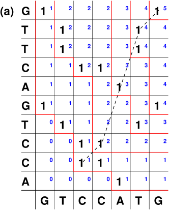
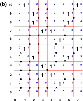
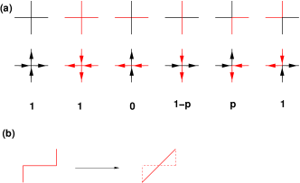
By construction, in the BM model each empty site has weight $q=1-p$, each left corner of each line has weight $p$, and all remaining sites have weight 1. This property allows for a mapping to a five-vertex model, see Fig. 1(b). For reasons that become apparent below we define this mapping slightly differently from MMN by interchanging the colour of all vertical lines. The resulting pattern of intersecting black and red lines then becomes isomorphic to the pattern of in- and outging arrows in the five-vertex model with vertex weights given by the weights of the BM model. One simply identifies black (red) horizontal lines with right-pointing (left-pointing) arrows and black (red) vertical lines with up-pointing (down-pointing) arrows as shown in Fig. 2(a).

Figure 2: (a) Mapping of line intersection to vertices of the six-vertex model which is effectively a five-vertex model since one of the vertex weights is zero. (b) A way to avoid line intersections in the five vertex model: if a horizontal line has a left adjacent vertical line below and a right vertical line above, it is replaced by the diagonal shortcut.

A similar terrace-like structure appears in the anisotropic 3D directed percolation model (ADP) solved by Rajesh and Dhar Dhar . A difference is that levels lines in the ADP can overlap. The overlapping lines can be separated by successive shifts of terraces, then one gets the five-vertex model with the same vertex weights as described above. However, the shifts destroy the domain-wall boundary conditions which are essential for thw exaxt solution of the BM model. Then, the analogy between the ADP and the BM models can be used only in the thermodynamic limit as it was demonstrated in MN .

It is useful to consider a further mapping of this 5-vertex model onto a discrete-time stochastic process, considering the vertical direction as time and horizontal one as discrete space. To this end, we first turn the red vertex lines (arrows pointing left or down) into non-intersecting particle world lines by replacing a right-left turn with a diagonal “shortcut”, as shown in Fig. 2(b). After a space reflection $i\to i^{\prime}=1-i$ this yields a non-intersecting line ensemble as shown in Fig. 3.

Figure 3: Mapping of the five-vertex model to non-intersecting worldlines after space reflection $i\to 1-i$. The green worldline is the first line (seen from the right) which does not reach the top of the grid.

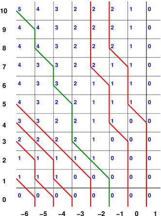
A final mapping is aimed to obtain the line ensemble of particle world lines of the discrete-time totally asymmetric exclusion process (TASEP) with the backward sequential update, introduced in backward and solved in Priezz . To this end, we consider each trajectory in Fig. 3 and replace each move upward by a diagonal move right and each diagonal move left by a move upward (Fig. 4). In a more formal way, we consider a new square lattice $(i^{\prime}+j+1/2,j)$ and draw new trajectories using the correspondence $(i^{\prime}+1/2,j)\rightarrow(i^{\prime}+j+1/2,j)$, see Fig. 4. The sites of the new lattice are denoted by coordinates $(k,t)$ numbered by integers $k=i^{\prime}+j$ and $t=j$. By construction the red lines move upward or diagonally and define the world lines of exclusion particles which jump only to the right. The vertex weights assign the appropriate probability to each path ensemble.

Figure 4: Worldlines of the TASEP. The space-time grid of the exclusion process is the square lattice $(i^{\prime}+j+1/2,j)$ with new coordinates $(k,t)$ numbered by integers $k=i^{\prime}+j$ and $t=j$. The green worldline is the first line (seen from the right) which does not reach the target position $(k,t)=(Y-X+1,Y)=(4,10)$ that yields $L_{X,Y}$ for $X=7,Y=10$.

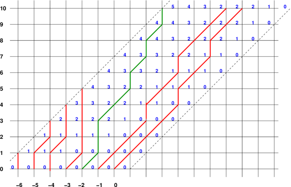
The backward sequential dynamics encoded in the vertex weights may be described as follows. In each time particle position are updated sequentially from right to left, starting from the rightmost particle. Each step of a particle by one lattice unit in positive direction has probability $1-p$, provided the neighbouring target site is empty. If the target site is occupied, the jump attempt is rejected with probability 1. No backward moves are allowed, making the exclusion process totally asymmetric. The horizontal boundary condition of the original sequence matching problem maps into an initial condition where at time $t=0$ particles occupy consecutive dual lattice points $-X+1\leq k\leq 0$. Since the motion of a particle is not influenced by any particles to its left, we may extend the lattice to minus infinity. The vertical boundary condition is equivalent to extending the lattice to plus infinity, such that at time $t=0$ all sites $k>0$ are vacant. Thus one has a TASEP on an initially half-filled infinite lattice with step initial state. However, only the first $X$ particles contribute to the statistical properties of the BM model.

In the exclusion picture the terrace height has a simple probabilistic interpretation. It counts the number of world lines that intersects with a diagonal in the square lattice starting from the point $(k,t)=(-x,0)$ (the left dotted line in Fig. 4. Hence, at any given time step, the terrace increases at each site from right to left by one unit, unless a world line has been crossed when going from right to left. Therefore the number $n$ of trajectories ending at time $t=Y$ and the length $L_{XY}$ of the LCS of the BM model on the rectangle $(X+1)\times(Y+1)$ are related by $L_{X,Y}=X-n$.

III Probability distribution of the LCS for finite sequences

Our aim is the evaluation of the probability distribution $\Lambda^{Q}_{XY}=\mbox{Prob}[L_{X,Y}=Q]$ of the Bernoulli model. Having the TASEP interpretation of the original model, we need to evaluate an appropriate sum over end points of trajectories of particles. To do this, we select the first trajectory (counted from the right) which does not end at time $Y$ in the target range of the dual lattice given by the top row $(i,Y$ with $1\leq i\leq X$ (the green line in Fig.4). An important observation is that the sum of weights of all trajectories ending at times $T_{1},T_{2},\dots T_{k}<Y$ (all lines to the left of the green line) is 1 for the conservation of probabilities in the TASEP. Then, the distribution $\Lambda^{Q}_{XY}$ is the sum over the probabilities of all trajectories with end points right of the green line and over end points of the green line itself. Hence of all $X$ particles only the rightmost $n+1=X-Q+1$ particles are relevant for the computation of $\Lambda^{Q}_{XY}$. The initial positions of these particles are $k_{1}=-X+Q,k_{2}=k_{1}+1,k_{3}=k_{2}+1,\dots,k_{n+1}=0$.

Following the relation between terrace height $Q$ and particle trajectories as discussed above, we may consider the final positions $x_{1},x_{2},\dots,x_{n+1}$ at the moment of time $Y$. By the construction, we have $Y-X+1\leq x_{2}<x_{3}<\dots<x_{n+1}\leq Y$ and $x_{1}\leq Y-X$. We first consider $Q=X$. In this case no particle has reached site $Y-X+1$. In particular, this implies that the first particle (initially at site $0$) has not reached site $Y-X+1$. The complementary probability for this event is the probability $P(Y-X+1,1,Y)$ that the first particle has jumped at least $Y-X+1$ times up to time $Y$. Hence

$$\Lambda_{X,Y}^{X}=1-P(Y-X+1,1,Y).$$ (3)

Now consider $Q<X$. Then $\Lambda^{Q}_{XY}$ is the joint probability that after $Y$ time steps all rightmost $X-Q$ particles (located initially on $(-X+Q+1,\dots,0)$) have reached sites $\geq Y-X+1$ and the next particle (located initially on $-X+Q$) has not reached site $Y-X+1$. This is equivalent to the joint probability that the particle originally at $-X+Q+1$ has jumped at least $Y-Q$ times and the particle originally at $-X+Q$ has jumped not more than $Y-Q$ times. By construction of the process this joint probability may be expressed as the statistical weight of all paths where the particle initially at $-X+Q+1$ jumps at least $Y-Q$ times minus the statistical weight of all paths where the particle initially at $-X+Q$ jumps at least $Y-Q+1$ times.

We have come to a known problem of the TASEP statistics Johansson ; RS . Consider an infinite chain, the left half of which is initially occupied by particles while the right half is empty. The problem is to find the probability $P(M,N,t)$ that the $N$th particle (counted from the right) of the infinite cluster hops at least $M$ times up to time $t$. With this quantity, we obtain for the partition function the expression

$$\Lambda_{X,Y}^{Q}=P(Y-Q,X-Q,Y)-P(Y-Q+1,X-Q+1,Y)$$ (4)

for every $Q<X$. For $Q=X$, Eq.(4) reduces to (3). We remark that Eq.(3) may be viewed as incorporated in Eq.(4) in agreement with the notion that the transition probability in an exclusion process with no particles (second argument of $P$ for $X+Q$) is equal to 1 (this is the trivial transition from the empty lattice to the empty lattice).

To derive Eq.(4) more formally, let $P(x_{1},x_{2},\dots,x_{n+1};k_{1},k_{2},\dots,k_{n+1}|t)\equiv P({\bf x^{(n+1)}};{\bf k^{(n+1)}}|t)$ be the probability that $n+1$ particles located initially at $k_{1},k_{2},\dots,k_{n+1}$ will be at $x_{1},x_{2},\dots,x_{n+1}$ at time $t$. Then, the partition function $\Lambda^{Q}_{XY}$ can be written as

$$\Lambda_{X,Y}^{Q}=\sum_{x_{n+1}=Y-Q}^{\infty}\dots\sum_{x_{2}=Y-X+1}^{x_{3}-1}\sum_{x_{1}\leq Y-X}P({\bf x^{(n+1)}};{\bf k^{(n+1)}}|Y)$$ (5)

Given the positions of $n$ particles at $x_{2},\dots,x_{n+1}$, the sum of conditional probabilities for the first particle to reach any position $x_{1}<x_{2}$ is

$$\sum_{x_{1}<x_{2}}P(x_{1}|x_{2},\dots,x_{n+1})\equiv\sum_{x_{1}<x_{2}}P(x_{1}|{\bf x^{(n)}})=1$$ (6)

and

$$\sum_{x_{1}\leq Y-X}P(x_{1}|{\bf x^{(n)}})=1-\sum_{x_{1}=Y-X+1}^{x_{2}-1}P(x_{1}|{\bf x^{(n)}})$$ (7)

The notations in (6) and (7) mean that probabilities to find a particle at $x_{1}$ with respect to positions of $n$ other particles, in contrast to probabilities $P({\bf x};{\bf k}|t)$ conditioned with respect to the initial conditions.

Using (7), we get the partition function in the form

$$\Lambda_{X,Y}^{Q}=\sum_{x_{n+1}=Y-Q}^{\infty}\dots\sum_{x_{2}=Y-X+1}^{x_{3}-1}P({\bf x^{(n)}};{\bf k^{(n)}})-\sum_{x_{n+1}=Y-Q+1}^{\infty}\dots\sum_{x_{1}=Y-X+1}^{x_{2}-1}P({\bf x^{(n+1)}};{\bf k^{(n+1)}})$$ (8)

where the time argument $Y$ is omitted. The probability $P({\bf x};{\bf k}|t)$ for the continuous time TASEP has been found in Schutz and for the discrete-time TASEP with the backward sequential update in Priezz :

$$P({\bf x};{\bf k}|t)=\det|F_{i-j}(x_{i}-k_{j};t)|$$ (9)

where

$$F_{m}(n;t)=\frac{1}{2\pi i}\int_{|z|=1-0}dz(p+\frac{q}{z})^{t}(1-z)^{-m}z^{n-1}$$ (10)

In terms of $P(M,N,t)$, the first sum in (8) is $P(Y-Q,X-Q,Y)$ and the second one is $P(Y-Q+1,X-Q+1,Y)$ which gives (4) again.

For the TASEP with parallel update $P(M,N,t)$ was computed by Johansson Johansson who used combinatorial methods of the theory of symmetric groups. For the present model with backward sequential update the solution was obtained by Rákos and Schütz using the Bethe ansatz method RS . For more general initial conditions, this problem has been solved by Nagao and Sasamoto Sasamoto . The expression for $P(M,N,t)$ obtained in RS by evaluation of sums of $P({\bf x};{\bf k}|t)$ reads

$$P(M,N,t)=\frac{q^{MN}(1-q)^{-MN+\frac{N(N+1)}{2}}}{\prod^{N}_{j=1}j!(M-j)!}\sum_{t_{1},t_{2},\dots,t_{N}=0}^{t-1}\{\prod_{j=1}^{N}\prod_{k=0}^{M-N-1}(t_{j}-k)(1-q)^{t_{j}}\}\prod_{i<j}(t_{i}-t_{j})^{2}.$$ (11)

where $q=1-p$ is the jump probability considered in RS . With (3) and (4) this gives the exact distribution of the LCS in the Bernoulli matching problem. The cumulative distribution

$$\Xi_{X,Y}^{Q}=\mbox{Prob}[L_{X,Y}\leq Q]=\sum_{M=0}^{Q}\Lambda_{X,Y}^{M}$$ (12)

takes the simple form

$$\Xi_{X,Y}^{Q}=P(Y-Q,X-Q,Y)$$ (13)

with the natural convention that $P(Y,0,Y)=1$. In RS it was shown explicitly that $P(Y-Q,X-Q,Y)=P(X-Q,Y-Q,X)$ which for the BM model is expected by symmetry. The result (13) provides a simple relation between the cumulative distribution of the length of the LCS in the BM model and the distribution of the time-integrated current in the backward-sequential TASEP for the step function initial condition. The probability that the length of the LCS is at most $Q$ is given by the probability that the number of jumps across bond $Y-X$ up to time $Y$ is at least $X-Q$.

IV Thermodynamic limit

We now turn to a brief discussion how the asymptotic results (2) of Sepp97 and MN follow from the cumulative distribution (13). To this end we need the asymptotic properties of $P(M,N,t)$ for large arguments. For parallel update Johansson has derived the asymptotics using results from the random matrix theory Johansson . By a transformation proved in RS this yields the asymptotics of the distribution $P(M,N,t)$ for the discrete time TASEP with the backward sequential update. One finds

$$\lim_{N\rightarrow\infty}P([\gamma N],N,N\omega(\gamma,q)+N^{1/3}\sigma(\gamma,q)\chi)=F_{GUE}(\chi)$$ (14)

with

$$\omega(\gamma,q)=\frac{(\sqrt{p}+\sqrt{\gamma})^{2}}{1-p}$$ (15)

and

$$\sigma(\gamma,q)=\frac{p^{1/6}}{\gamma^{1/6}}\frac{(\sqrt{p}+\sqrt{\gamma})^{2/3}(1+\sqrt{p\gamma})^{2/3}}{1-p}$$ (16)

The function $F_{GUE}(\chi)$ is the Tracy-Widom distribution of the Gaussian unitary ensemble TW .

The form of (14) indicates that given $N$ and $\gamma$, the non-trivial scaling regime in time is given by the third argument. In the present case, $t=Y$ and $\gamma$ are fixed and we search for the scaling regime of $Q$. In our notations, $M=Y-Q$, $N=X-Q$, $t=Y$ and $\gamma=(Y-Q)/(X-Q)$. From Eq.(14) we have

$$Y\sim(X-Q)\omega(\gamma,q)+(X-Q)^{1/3}\sigma(\gamma,q)\chi$$ (17)

To find the asymptotics of $Q$ for large $X$ and $Y$, we represent it in the form

$$Q(X,Y,q)=Q_{0}(X,Y,q)+R(X,Y,q)\chi$$ (18)

Then, the leading term $Q_{0}(X,Y,q)$ can be found from the equation

$$Y=\frac{X-Q_{0}(X,Y,q)}{1-p}\left(\sqrt{p}+\frac{\sqrt{Y-Q_{0}(X,Y,q)}}{\sqrt{X-Q_{0}(X,Y,q)}}\right)^{2}$$ (19)

which gives

$$Q_{0}(X,Y,q)=\frac{2\sqrt{pXY}-p(X+Y)}{1-p}$$ (20)

which coincides with the expression found by Seppäläinen Sepp97 using probabilistic methods.

The substution of Eq.(18) with Eq.(20) into Eq.(17) leads to the equation for $R(X,Y,q)$ which can be resolved in the leading order of $\chi$. In the first order, we substitute $Q=Q_{0}$ into the second term of the RHS of Eq.(17) to get

$$(X-Q_{0})^{1/3}\sigma(\gamma_{0},q)=\left(\frac{\sqrt{p}XY}{(\sqrt{X}-\sqrt{pY})(\sqrt{Y}-\sqrt{pX})}\right)^{1/3}$$ (21)

where

$$\gamma_{0}=\frac{Y-Q_{0}}{X-Q_{0}}$$ (22)

The coefficient $c_{1}$ at $R(X,Y)\chi$ in the expansion of the first term of the RHS of Eq.(17) is

$$c_{1}=\frac{(1-p)\sqrt{XY}}{(\sqrt{X}-\sqrt{pY})(\sqrt{Y}-\sqrt{pX})}$$ (23)

Then, $R(X,Y,q)$ is the ratio $(X-Q_{0})^{1/3}\sigma(\gamma_{0},q)/c_{1}$ and we obtain

$$R(X,Y,q)=\left(\frac{p}{XY}\right)^{1/6}\frac{(\sqrt{X}-\sqrt{pY})^{2/3}(\sqrt{Y}-\sqrt{pX})^{2/3}}{1-p}$$ (24)

Both results Eq.(20) and Eq.(24) coincide with corresponding expressions obtained in MN from a comparison with Johansson’s result for the directed polymer problem Johansson .

V Conclusions

We have considered the Bernoulli matching model of sequence alignment with the aim of deriving the exact probability that longest common subsequence of two sequences of finite lengths $X,Y$ has length $N$. By a series of mappings we have transformed the matching problem to the time evolution of the totally asymmetric simple exclusion process with backward sequential update in a step-function initial state. In this mapping the computation of the probability distribution turns into the distribution of the time-integrated current through a certain bond. This problem has been solved by Rákos and Schütz RS by Bethe ansatz methods. Thus the desired result for the Bernoulli matching model for finite sequences has been obtained in explicit form (13) through some coordinate transformations from the Bethe ansatz.

In the thermodynamic limit we recover the earlier results of Majumdar and Nechaev MN through an asymptotic analysis where we use the fact that in the thermodynamic limit there is a scaling form of the current distribution found by Johansson Johansson which involves the distribution of the largest eigenvalue of the GUE ensemble of random matrices. Adapting this result to the present setting requires again some nontrivial coordinate transformation. We find the occurrence of an eigenvalue distribution of random matrices (which is valid also for finite sequence lengths, but for the Laguerre ensemble) intriguing.

VI Acknowledgements

We thank S.Nechaev, S. Majumdar and K. Mallick for many useful discussions. We acknowledge the support of the DFG. V.P. appreciates also the support of the RFBR grant No. 06-01-00191a. Part of this work was done while G.M.S. was the Weston Visiting Professor at the Weizmann Institute of Science.

References

- (1) D. Sankoff and J. Kruskal, Time Warps, String Edits, and Macromolecules: The theory and practice of sequence composition (Addison Wesley, Reading,Massachussets, 1983).
- (2) M.S. Waterman, Introduction to Computational Biology (Chapman and Hall, London, 1994).
- (3) D. Gusfield, Algorithms on Strings,Trees, and Sequences (Cambridge University Press, Cambridge, 1997).
- (4) J. Boutet de Monvel, Eur. Phys. J. B 7, 293 (1999); Phys. Rev. E 62, 204 (2000).
- (5) T. Seppäläinen, Ann. Appl. Probab. 7, no. 4, 886 (1997).
- (6) S.N. Majumdar and S. Nechaev, Phys. Rev. E 72, 020901(R) (2005).
- (7) S.N. Majumdar, K. Mallick and S. Nechaev, arXiv:0710.1030v1 [cond-mat.stat-mech](2007).
- (8) R.Bundschuh, Phys. Rev. E 65, 031911 (2002).
- (9) R.Bundschuh and T.Hwa, Discrete Appl. Math. 104, 113 (2000).
- (10) N. Rajewsky, A. Schadschneider, and M. Schreckenberg, J.Phys. A 29,L305 (1996).
- (11) K. Johansson, Commun. Math. Phys. 209, 437 (2000).
- (12) R.Rajesh and D.Dhar, Phys.Rev. Lett. 81, 1646 (1998).
- (13) A. Rákos and G.M. Schütz J. Stat. Phys. 118, 511 (2005).
- (14) T. Nagao and T. Sasamoto, Nucl. Phys. B 699,487 (2004).
- (15) G.M. Schütz, J. Stat. Phys. 88,427 (1997).
- (16) V.B. Priezzhev, in Proceedings Statphys 22 Pramana-J.Phys. 64, 915 (2005); cond-mat/0211052 (2002).
- (17) C.A. Tracy and H. Widom, Commun. Math. Phys. 159, 151 (1994); 177, 727(1996).