Chaotic motion of Charged Particles in an Electromagnetic Field Surrounding a Rotating Black Hole

Abstract

The observational data from some black hole candidates suggest the importance of electromagnetic fields in the vicinity of a black hole. Highly magnetized disk accretion may play an importance rule, and large scale magnetic field may be formed above the disk surface. Then, we expect that the nature of the black hole spacetime would be reveiled by magnetic phenomena near the black hole. We will start to investigate the motion of a charged particle which depends on the initial parameter setting in the black hole dipole magnetic field. Specially, we study the spin effects of a rotating black hole on the motion of the charged particle trapped in magnetic field lines. We make detailed analysis for the particle’s trajectories by using the Poincaré map method, and show the chaotic properties that depend on the black hole spin. We find that the dragging effects of the spacetime by a rotating black hole weaken the chaotic properties and generate regular trajectories for some sets of initial parameters, while the chaotic properties dominate on the trajectories for slowly rotating black hole cases. The dragging effects can generate the fourth adiabatic invariant on the particle motion approximately.

1 Introduction

In the central region of AGNs, compact X-ray sources and GRBs, many black hole candidates are reported. The observational data from their active regions would include the informations about the gravitational and electromagnetic fields. However, there are no direct observational evidences for the existence of a black hole in the center of the compact active regions. So, it is very important how to find the informations on the curved spacetime from observational data, and how to interpret their nature. Although the inner part of a gas disk around a supermassive black hole emits non-thermal radiation, this may be explained by synchrotron emission from ultra-relativistic electrons in strong magnetic field regions around a black hole. In the central black hole system, however, the emission process is very little understood, although the consensus is in favor of emission due to plasma process. The emission from such particles would give us the information about the black hole spacetime and/or the electromagnetic field.

In a realistic model of a black hole–disk system, we should consider interactions between a plasma particle and a magnetic field in the curved spacetime. The plausible electromagnetic field around a black hole–disk system is still unknown, although some authors have discussed this problem in the frame work of magnetohydrodynamics (e.g., Blandford & Znajek, 1977; Camenzind, 1987; Nitta, Takahashi, & Tomimatsu, 1991; Tomimatsu & Takahashi, 2001). In general, the task for solving the structure of magnetic fields in a black hole system is very hard. Then, to make a comprehensive analysis, we will give a vacuum external magnetic field around a rotating black hole, and investigate in detail the motion of a charged particle confined in the magnetic field. The stationary and axisymmetric vacuum electromagnetic fields around a black hole are discussed by Petterson (1975); Chitre & Vishveshwara (1975); Li (2000); Ghosh (2000); Tomimatsu & Takahashi (2001). We apply the black hole dipole magnetic field in Kerr geometry, which is a solution of the vacuum Maxwell’s equations. Although the dipole magnetic field could correspond to the intrinsic field of a compact object like a neutron star, in the case of black holes it has to results from current rings exterior to the event horizon but they can be very close to it (Prasanna, 1978). As known in the Earth’s magnetosphere, the dipole magnetic field can trap charged particles within its magnetic bottle (i.e., the Van Allen belts). The particle gyrates around the magnetic field line, and drifts in the toroidal direction (see, e.g., Goedbloed & Poedts, 2004). Furthermore, in the poloidal plane, the particle oscillates along the magnetic field line. In the black hole case, we can also expect similar situations.

In a black hole magnetosphere, by solving equations of motion of a charged particle moving in the electromagnetic field numerically (see Prasanna, 1978), we can see the gyration around the magnetic field line, the drift in the toroidal direction and the multi-periodic motion in the poloidal plane. Such a orbit is very complicated in both poloidal and toroidal directions. Although a stationary and axisymmetric magnetosphere is assumed, there are two conserved quantities; that is, the energy and angular momentum of the charged particle. In addition to these, the rest mass of the particle is the third invariable quantity. However, the fourth invariable quantity related to the azimuthal motion of the particle does not exist when the electromagnetic field is considered around a black hole. Thus, the motion of a test charge in a black hole magnetosphere is not an integrable system. Then, the chaotic motion is expected (Nakamura & Ishizuka, 1993). To examine the trajectory, we plot the Poincaré map in the two-dimensional $r$-$p^{r}$ plane, which shows intersections of the particle’s trajectories with the surface of section in phase space (Lichtenberg & Liberman, 1992). If the plotted points form a closed curve, the motion is regular (not chaotic). This is because a regular trajectory moves on a torus in the phase space and the curve is a cross section of the torus. On the other hand, if the plotted points are distributed randomly, the motion is irregular (chaotic). From the distribution of the points in the Poincaré map, we can judge whether or not the motion is chaotic. Then, we know chaotic behavior on the trajectory of a charged particle in a black hole magnetosphere. Furthermore, we find the black hole’s spin effects on that chaotic motion.

This study will be related to the source of radiation near a black hole. We will start this work as a basic step before considering the plasma as a magnetized fluid. Although we find chaotic and/or regular motion in a black hole magnetosphere, the problem is how to find the phenomena in the observed spectrum. At this stage, however, we can not show the relation with the observational data in this work. The main purpose of this study is to understand the black hole spin effects (the dragging effects by a rotating black hole) on a test charge, which will be considered as the source plasma of high energy radiation in future.

In § 2, we review the basic equations for the motion of a charged particle in a black hole magnetosphere, using the Hamilton-Jacobi formalism. To understand the nature of orbits of a charged particle in the black hole magnetosphere, we also consider in § 3 the effective potential including the four-vector potential of the magnetic field. We present the motions of a test charge in the black hole dipole magnetic field for various values of black hole’s spin parameters. In § 4 we make detailed analysis for its trajectories by using the Poincaré map method, and show the chaotic properties that depend significantly on the black hole spin obviously. We see simultaneous presence of regular trajectories and regions of stochastic trajectories on the Poincaré map. Furthermore, we find that due to the dragging effects of a rapidly rotating black hole, the fourth constant of motion approximately turns out to exit. Then, the motion of a test charge in a dipole magnetic field around a rotating black hole can behave like a integrable system.

2 Equations for a Charged particle around a Black Hole

We study the motion of a relativistic charged particle with the rest mass $m$ and charge $q$ in Kerr geometry. The background metric is written by the Boyer-Lindquist coordinates ($t,r,\theta,\phi$) with $c=G=1$, where the signature of the metric is $-2$. The non-zero components of the contravariant metric $g^{\mu\nu}$ are given by

$$g^{tt}=\frac{A}{\Delta\Sigma}\ ,~{}~{}~{}g^{t\phi}=\frac{2Mar}{\Delta\Sigma}\ ,~{}~{}~{}g^{\phi\phi}=-\frac{1-2Mr/\Sigma}{\Delta\sin^{2}\theta}\ ,~{}~{}~{}g^{rr}=-\frac{\Delta}{\Sigma}\,~{}~{}~{}g^{\theta\theta}=-\frac{1}{\Sigma}\ .$$ (1)

where $\Sigma\equiv r^{2}+a^{2}\cos^{2}\theta$, $\Delta\equiv r^{2}-2Mr+a^{2}$, $A\equiv(r^{2}+a^{2})^{2}-\Delta a^{2}\sin^{2}\theta$. The external electromagnetic field is assumed to be stationary and axisymmetric. We assume that the electromagnetic fields would not disturb the background geometry of the spacetime. In fact the electromagnetic fields seen in astrophysical black hole candidates would be quite small compared with the gravitational field associated with the black hole.

The Hamiltonian of the system can be defined as (e.g., Misner, Thorne & Wheeler, 1973)

$$H\equiv\frac{1}{2}g^{\mu\nu}(\pi_{\mu}-qA_{\mu})(\pi_{\nu}-qA_{\nu})$$ (2)

where $\pi_{\mu}$ is the canonical momentum and $A_{\mu}=A_{\mu}(r,\theta)$ is the four-vector potential of the electromagnetic field. The four-momentum of a charged particle is

$$p^{\mu}\equiv\frac{dx^{\mu}}{d\lambda}=g^{\mu\nu}(\pi_{\nu}-qA_{\nu})\ ,$$ (3)

where $\lambda=\tau/m$ is an affine parameter and $\tau$ is the proper time. The Lorentz-force equation is equivalent to Hamilton’s equations written in terms of $x^{\mu}$ and $\pi_{\mu}$:

$$\frac{dx^{\mu}}{d\lambda} = \frac{\partial H}{\partial\pi_{\mu}}\ ,$$ (4)

$$\frac{d\pi_{\mu}}{d\lambda} = -\frac{\partial H}{\partial x^{\mu}}\ .$$ (5)

In a stationary and axisymmetric black hole magnetosphere, the magnetic field is specified by a scalar function $\Psi$ of position called the stream function; that is, the poloidal magnetic field lines are contours of constant $\Psi$. (The function $\Psi$ is proportional to the toroidal component of the vector potential, $A_{\phi}$.) In this paper we set up a vacuum magnetosphere, so that no total poloidal current exists, and then the toroidal component of the magnetic field is zero.

From the stationary and axial symmetry of both electromagnetic field and spacetime geometry, $E\equiv\pi_{t}=p_{t}+qA_{t}$ and $L\equiv-\pi_{\phi}=-(p_{\phi}+qA_{\phi})$ are constants of motion corresponding to the integrable coordinates $t$ and $\phi$ in eq. (2). The third constant of motion is the particle’s rest mass $m=(-g^{\mu\nu}p_{\mu}p_{\nu})^{1/2}$. In general, four constants of motion are needed to determine uniquely the orbit of a particle through four-dimensional spacetime. However, a test charge motion in a magnetic field around a black hole posses only three obvious constants. So we can expect chaotic behavior for its motions (Lichtenberg & Liberman, 1992; Karas & Vokrouhlick’y, 1992), because such a system is non-integrable. Note that, without the magnetic field, the fourth constant of motion exists. This constant is known as Carter’s constant of the motion

$${\cal Q}=p_{\theta}^{2}+\cos^{2}\theta\left[a^{2}(m^{2}-E^{2})+\frac{L^{2}}{\sin^{2}\theta}\right]\ ,$$ (6)

which arises as a separation-of-variables constant in the Hamilton-Jacobi derivation of equation of motion (see Misner, Thorne & Wheeler, 1973). That is, the motion of a test particle in Kerr spacetime without magnetic field is an integrable system.

The stationary and axisymmetric electromagnetic fields around a rotating black hole in source-free regions are derived by Petterson (1975). Here, we consider the solution that denotes dipole magnetic fields at distant regions, and call this solution “black hole dipole electromagnetic field”. In this black hole magnetosphere, we expect that the dipole magnetic field configuration can trap a charged particle within their magnetic bottle, even if it extends close to the black hole. The four-vector potential of the black hole dipole has only two nonzero components, $A_{t}$ and $A_{\phi}$; the dipole magnetic field and an induced quadrupole electric field in Kerr geometry are given by

$$A_{t} = \frac{-3a\mu}{2\gamma^{2}\Sigma}\left\{\left[r(r-M)+(a^{2}-Mr)\cos^{2}\theta\right]\frac{1}{2\gamma}\ln\left(\frac{r-r_{-}}{r-r_{+}}\right)\right.$$ (7)

$$~{}~{}~{}~{}~{}~{}~{}~{}-(r-M\cos^{2}\theta)\bigg{\}}~{}\ ,$$

$$A_{\phi} = \frac{-3\mu\sin^{2}\theta}{4\gamma^{2}\Sigma}\bigg{\{}(r-M)a^{2}\cos^{2}\theta+r(r^{2}+Mr+2a^{2})$$ (8)

$$~{}~{}~{}~{}~{}~{}~{}-\left[r(r^{3}-2Ma^{2}+a^{2}r)+\Delta a^{2}\cos^{2}\theta\right]\frac{1}{2\gamma}\ln\left(\frac{r-r_{-}}{r-r_{+}}\right)\bigg{\}}\ ,$$

where $\gamma\equiv(M^{2}-a^{2})^{1/2}$, $r_{\pm}=M\pm\gamma$ and the dipole moment $\mu$ is taken to be anti-parallel to the rotation axis. In the $a\to M$ limit, we obtain

$$A_{t} = \frac{-M\mu[r\sin^{2}\theta-2(r-M)\cos^{2}\theta]}{2(r^{2}+M^{2}\cos^{2}\theta)(r-M)^{2}}\ ,$$ (9)

$$A_{\phi} = \frac{-\mu\sin^{2}\theta[-2r^{3}+M(r-M)(r+M\cos^{2}\theta)]}{2(r^{2}+M^{2}\cos^{2}\theta)(r-M)^{2}}\ .$$ (10)

In the limit of $a\to M$, $|A_{t}|$ and $|A_{\phi}|$ diverge as $(r-M)^{-2}$, while in the case of $a<M$, $|A_{t}|$ and $|A_{\phi}|$ diverge logarithmically at the event horizon. Although the source of the magnetic field should be outside the event horizon, the current loops could locate just outside the event horizon (arbitrarily close to it) as the source of such dipole magnetic fields as considered in this work (Prasanna, 1978). In spite of this singularity, we will use this configuration for the study of the chaotic motion of a test charge around a black hole. The appearance of the singularity does not imply that the dipole field is invalid. It is valid in the regions considered outside the event horizon. In a realistic situation for the black hole magnetosphere as an astrophysical model, to avoid the singularity at the event horizon, the infinite sum of multi-pole fields is necessary (Li, 2000; Tomimatsu & Takahashi, 2001). The plausible magnetic field configuration around a black hole should be investigated as a future work.

3 Orbits of a charged particle in a magnetosphere

Now, we will discuss charged particle motions off the equatorial plane of the black hole dipole field. The concrete expressions of equations (4) and (5) including electromagnetic field terms are very complicated, and are not particularly informative. However, by considering an effective potential in the poloidal plane, we can get a general picture of the orbits, although we need to integrate the equations of motion numerically to obtain the practical orbits.

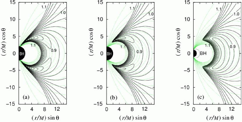
Figure 1: Effective potential with the black hole dipole magnetic field (thin gray curves). (a) $a=0.0$, (b) $a=0.3M$ and (c) $a=M$, where $L/m=-7.0M$ and $Q_{d}=70.0M^{2}$. In these plots, the maximum level of $V_{\rm eff}$ is 1.1 and the interval is 0.02.

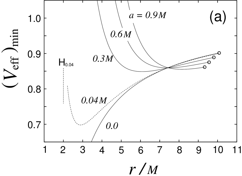
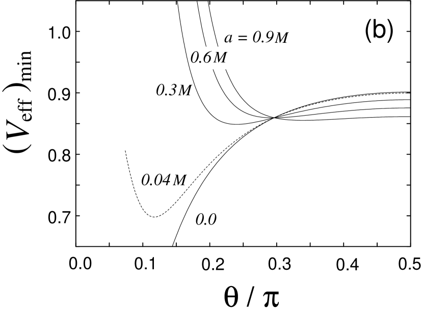
Figure 2: Potential valley for various spin values. (a) $(V_{\rm eff})_{\rm min}$ vs. $r$ and (b) $(V_{\rm eff})_{\rm min}$ vs. $\theta$ are plotted, where $L/m=-7.0M$ and $Q_{d}=70.0M^{2}$. The circles in (a) indicate $\theta=\pi/2$, and the vertical line labeled by H_0.04 shows the event horizon for $a=0.04M$.

Here, we consider off-equatorial motion for a charged particle in the dipole magnetic field. By using the condition $g^{\mu\nu}p_{\mu}p_{\nu}=m^{2}$ with the constants of motion $E$ and $L$, the equation of motion in the poloidal plane can be obtained. Then, without the kinetic terms of the poloidal motion ($p^{r}=p^{\theta}=0$), we can define the effective potential (Esteban & Medina, 1990) as

$$V_{\rm eff}(r,\theta)\equiv\frac{E_{\rm min}}{m}=\frac{q}{m}A_{t}+\frac{g^{t\phi}}{g^{tt}}\left(\frac{L}{m}+\frac{q}{m}A_{\phi}\right)+\frac{1}{g^{tt}}\left[\frac{1}{\rho_{w}^{2}}\left(\frac{L}{m}+\frac{q}{m}A_{\phi}\right)^{2}+g^{tt}\right]^{1/2}\ ,$$ (11)

where $E_{\rm min}$ is the allowed minimum energy for a particle at the injection point. Although the distribution of the effective potential depends on the value of $L/m$ and $q/m$ of the charged particle and the electromagnetic field configuration $A_{t}$ and $A_{\phi}$, to study the chaotic behavior we are interested in the case that a charged particle is trapped in a bound orbit. When the energy of a charged particle is not so large ($V_{\rm eff}<E/m<1$), the particle is bound in the orbit in the region of the potential well. That is, the particle has turning points, which correspond to the inner and outer envelope of the Larmor motion in the poloidal plane.

The detailed motion in the equatorial plane ($p^{\theta}=0$) in the Kerr background with the dipole magnetic field has been discussed by Prasanna (1980). We will also see the projection onto the equatorial plane of the off-equatorial particle’s motions. From the $\phi$-component of the equation of motion, we obtain

$$p^{\phi}=g^{t\phi}(E-qA_{t})-g^{\phi\phi}(L+qA_{\phi})\ .$$ (12)

For a non-rotating black hole case, the first term is negligible. When the signatures of parameters $L$ and $q\mu$ are same, the particle does not gyrate because of $p^{\phi}\neq 0$. To observe the gyration motion of a charged particle, where $p^{\phi}=0$ is achieved periodically, we will choose $L<0$ and $Q_{d}\equiv(q/m)\mu>0$ in the following numerical calculations. To see the off-equatorial motion of a charged particle, the initial value of $p^{r}$ or $p^{\theta}$ should be specified. In this paper, we inject the particle into the magnetosphere with the injection angle $\psi_{\rm inj}$, which is the angle from the origin of the coordinate axes in the poloidal plane and is relate to the ratio of the initial $p^{r}$ and $p^{\theta}$-values, where we choose $0<\psi_{\rm ini}<0.5\pi$ for the calculations. The label “ini” indicate the quantity at the injection point. The equations are solved by using the 4th-order Runge-Kutta-Gill method.

Figure 1 shows the hole’s spin dependence on the effective potential $V_{\rm eff}(r,\theta)$ for the poloidal motion of a charged particle in the black hole dipole magnetic field. We see the valley-like structure in the lower-level potential region (named “potential valley”), which is across the northern and southern hemispheres nearly along a dipole magnetic field line, wherein the particle with lower energy can be trapped inside it. We also see a divide of the potential valley just on the equatorial plane, Figure 2 shows the $r$- and $\theta$-dependences of the local minimum of the effective potential in the $r$-direction, which is obtained from $\partial V_{\rm eff}(r,\theta)/\partial\theta=0$ and corresponds to the bottom along the valley, for various values of the spin parameter $a$. In this plot, we see the local minimum in the middle-latitude region in the $\theta$-direction.

In the non-rotating black hole case (see Fig. 1a), the value of the local minimum of the effective potential decreases from the equator to the event horizon along almost the dipole magnetic field line in both hemispheres, and has the minimum value at the event horizon. Thus, the potential valley is opened toward the black hole, while the width of the valley becomes narrower toward the event horizon. So, although a particle can be trapped within the potential valley for some time, the particle will fall into the black hole sooner or later. Figure 3 is an example of the orbit for a non-rotating black hole, where the projection on the equatorial plane (left panel) and the poloidal motion (right panel) are shown. The particle gyrates around the magnetic field line, and drifts in the toroidal direction. Furthermore, the particle oscillates in the poloidal plane along the magnetic field lines. In this dipole magnetic field case, the particle entering the regions of higher magnetic field strengths reflects back into the regions of smaller magnetic field strength. This is the so-called “mirror effects”. Although the dipole field traps a particle between two mirrors, the particle falls into the black hole in the end, for almost non-rotating black hole cases. In Figure 3 we show the case of $\psi_{\rm inj}=-0.16\pi$, but it is easy to fall into the black hole sooner for the larger value of $\psi_{\rm inj}$.

Next, for a rotating black hole case (see Fig. 1b), the centrifugal barrier by the hole’s spin effects arises and the potential valley is disconnected from the event horizon. This is because the centrifugal barrier due to the hole’s spin becomes higher with increasing the black hole spin. Thus, the dragging effects of spacetime enhance the mirror effects. Then, the particle can be trapped within the potential valley without falling onto the black hole. Furthermore, we see the “double-well potential” along the valley. Basically, the particle oscillates between the northern and southern hemispheres, but sometimes a particle with lower energy may be trapped in one hemisphere. Such a double-well potential may be related to the chaotic motion as discussed later. For the extreme rotating case shown in Fig. 1c, the spin effects are more effective. We see an almost single-well potential along the valley. Then, we can expect that the particle would oscillate between the northern and southern hemispheres periodically. The trajectory for the particle trapped in the potential valley will be discussed in §5 again.

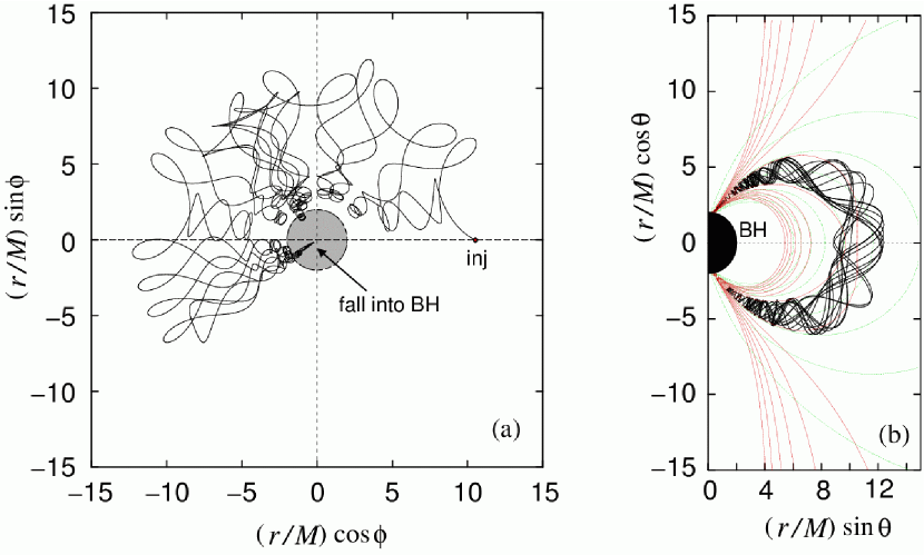
Figure 3: The motion of a charged particle in the equatorial plane (LEFT) and in the poloidal plane (RIGHT). The particle finally falls into the event horizon from the polar region of the black hole. The parameters of the motion are given as $a=0$, $E/m=0.920$, $Q_{d}=70M^{2}$, $\psi_{\rm ini}=-0.16\pi$, $x_{\rm ini}=10.5M$ and $\theta_{\rm ini}=\pi/2$. In the poloidal plane, the dipole magnetic field lines (thin gray curves) and the effective potential (thin curves) are also plotted.

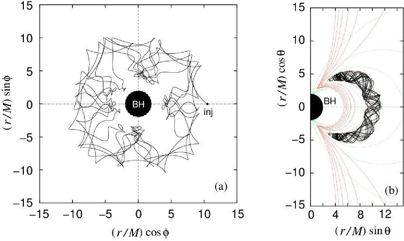
Figure 4: An Example of the random trajectory of a test charge. LEFT panel shows the projections on the equatorial plane, and RIGHT panel shows the projections on the poloidal plane. The parameters of the motion are set as $a=0.3M$, $E/m=0.900$, $\psi_{\rm ini}=-0.20\pi$, $L/m=-7.0M$, $Q_{d}=70.0M^{2}$, $r_{\rm ini}=10.5M$ and $\theta_{\rm ini}=\pi/2$.

Figures 4–6 show the orbits of a charged particle around a rotating black hole. Charged particles are trapped within the potential valley (i.e., a magnetic bottle) without falling onto a black hole. So, we can carry out long-time calculations for chaos studies. The particle oscillates quasi-periodically between the northern and southern hemisphere, although it is a very complicated orbit. In Figures 4, 5(TOP) and 6(BOTTOM), the particle’s orbit seems to be random, while in Figure 5(BOTTOM) and 6(TOP), the orbit looks regular; that is, we can see some kind of periodicity despite its long-time motion. For rapidly rotating cases, we can see the regular orbits often in comparison with the slowly rotating cases. In general, some orbits show a regular trajectory, while a chaotic trajectory still remains. Thus, we can find spin effects on the motion of the charged particle. In the following, we analyze the detailed properties of these motions to clarify their dependence on the spin parameter. Such motions may be chaotic. So, we analyze the properties of the motions using a method with which we analyze chaotic behavior.

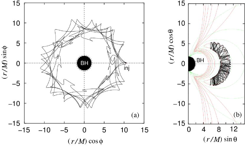
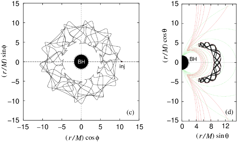
Figure 5: Examples of the trajectories of a test charge for $a=0.6M$. LEFT column shows the projections on the equatorial plane, and RIGHT column shows the projections on the poloidal plane. The parameters of the motion are set as (a,b) $E/m=0.895$, $\psi_{\rm ini}=-0.10\pi$, (c,d) $E/m=0.890$, $\psi_{\rm ini}=-0.30\pi$, with $L/m=-7.0M$, $Q_{d}=70.0M^{2}$, $r_{\rm ini}=10.5M$ and $\theta_{\rm ini}=\pi/2$.

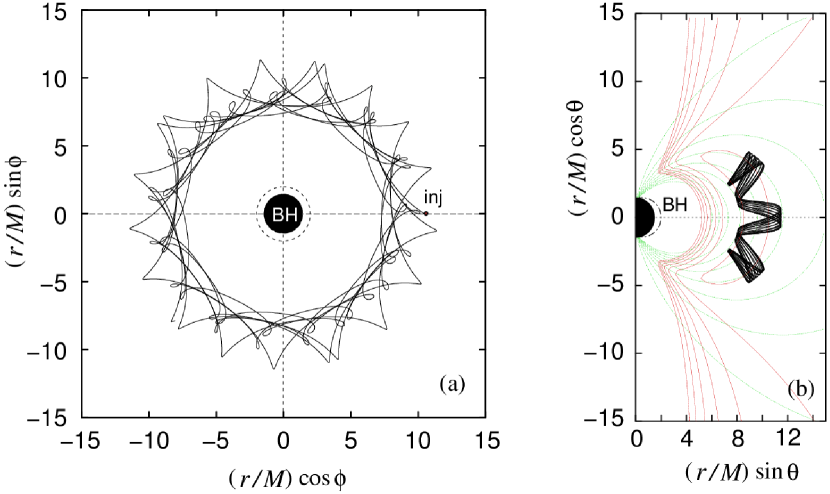
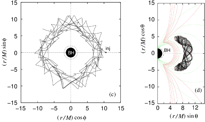
Figure 6: Examples of the trajectories of a test charge for $a=0.9M$. LEFT column shows the projections on the equatorial plane, and RIGHT column shows the projections on the poloidal plane. The parameters of the motion are set as (a,b) $E/m=0.885$, $\psi_{\rm ini}=-0.10\pi$, (c,d) $E/m=0.885$, $\psi_{\rm ini}=-0.22\pi$, with $L/m=-7.0M$, $Q_{d}=70.0M^{2}$, $r_{\rm ini}=10.5M$ and $\theta_{\rm ini}=\pi/2$.

4 Regular and Chaotic orbits

The particle motions are common in the sense that they are the combinations of three types of motions (gyration, bouncing, and drifting). Here we analyze the property of such complicated motions using the Poincaré map, which shows intersections of a trajectory with the surface of section in phase space. The motion of a point in phase space could be followed over hundreds of thousands of oscillation periods. The Poincaré map is an useful tool to classify visually whether the motions are regular (non chaotic) or irregular (chaotic). To make the Poincaré map, we adopt the equatorial plane ($\theta=\pi/2$) as a Poincaré surface and plot the point ($r$, $p^{r}$) when the particle crosses the Poincaré section with ($p^{\theta}>0$). We obtain that, for a slowly rotating black hole case, a trajectory plots a lot of points on the map randomly, while for a rapidly rotating case there are some regular trajectories shown by tori. The different tori indicate the different initial injection angle $\psi_{\rm ini}$ on the Poincaré map. The appearance of regular trajectories suggests that the dragging effects of the black hole generate a nearly integrable system in spite of the existence of a magnetic field in Kerr spacetime (the details will be discussed in § 5).

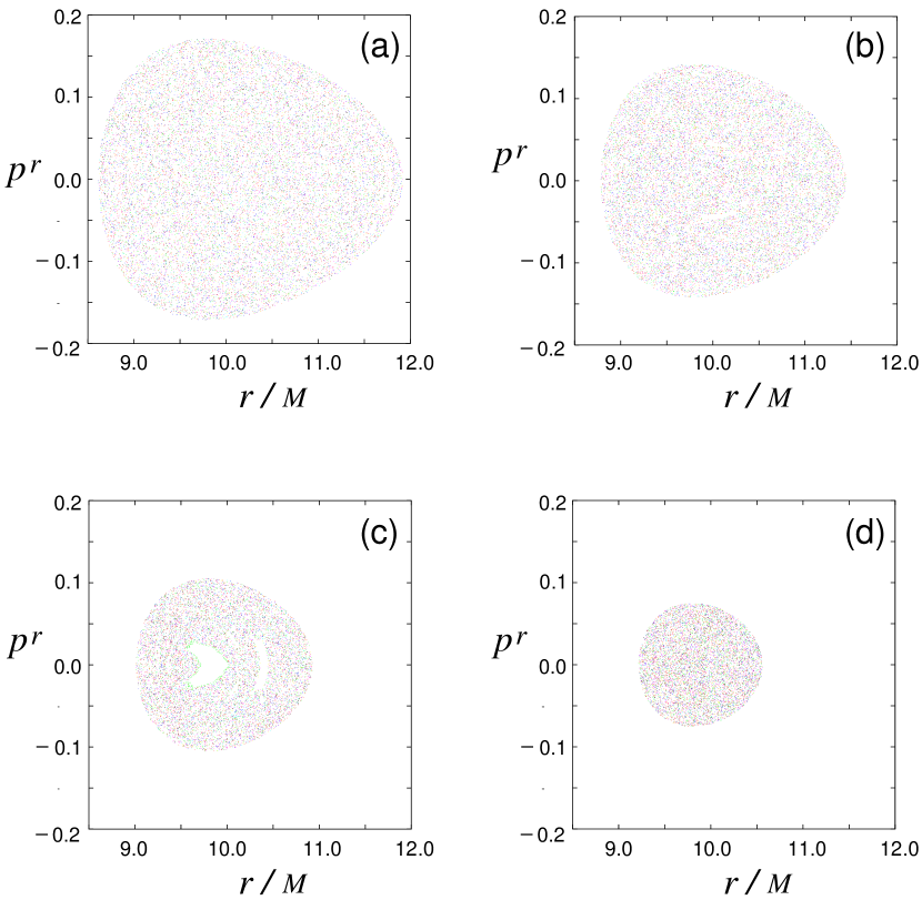
Figure 7: The Poincaré map of a charged particle orbiting in the dipole magnetic field around a black hole of $a=0.3M$. The intersections are shown by small dots on the map. The parameters for the motion are (a) $E/m=0.905$, (b) $E/m=0.900$, (c) $E/m=0.895$ and (d) $E/m=0.892$ with $L/m=-7.0M$, $Q_{d}=70.0M^{2}$, $r_{\rm ini}=10.5M$ and $\theta_{\rm ini}=\pi/2$.

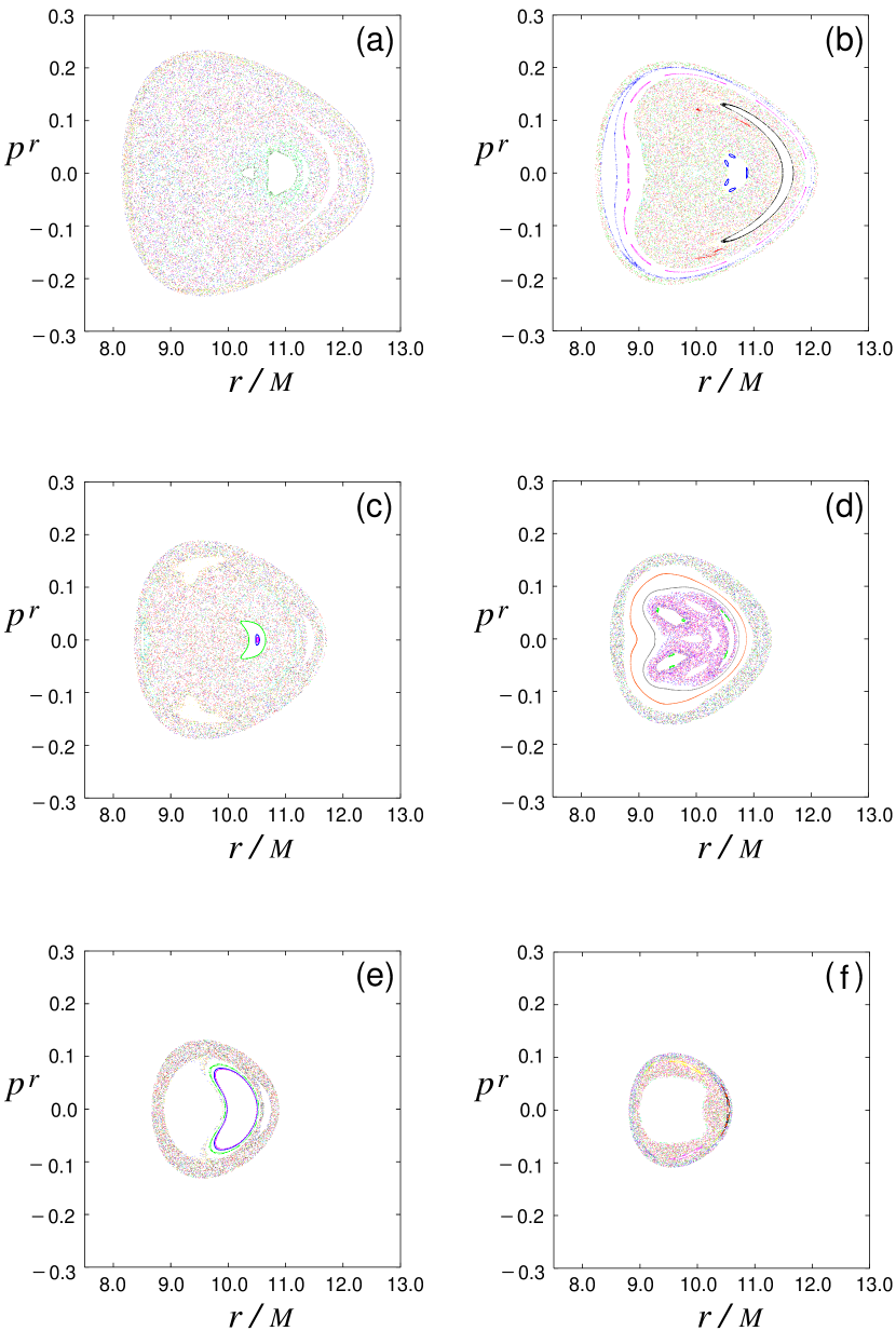
Figure 8: The Poincaré map of a charged particle orbiting in the dipole magnetic field around a black hole of $a=0.6M$. The parameters for the motion are (a) $E/m=0.905$, (b) $E/m=0.900$, (c) $E/m=0.895$, (d) $E/m=0.890$, (e) $E/m=0.885$ and (f) $E/m=0.882$ with $L/m=-7.0M$, $Q_{d}=70.0M^{2}$, $r_{\rm ini}=10.5M$ and $\theta_{\rm ini}=\pi/2$.

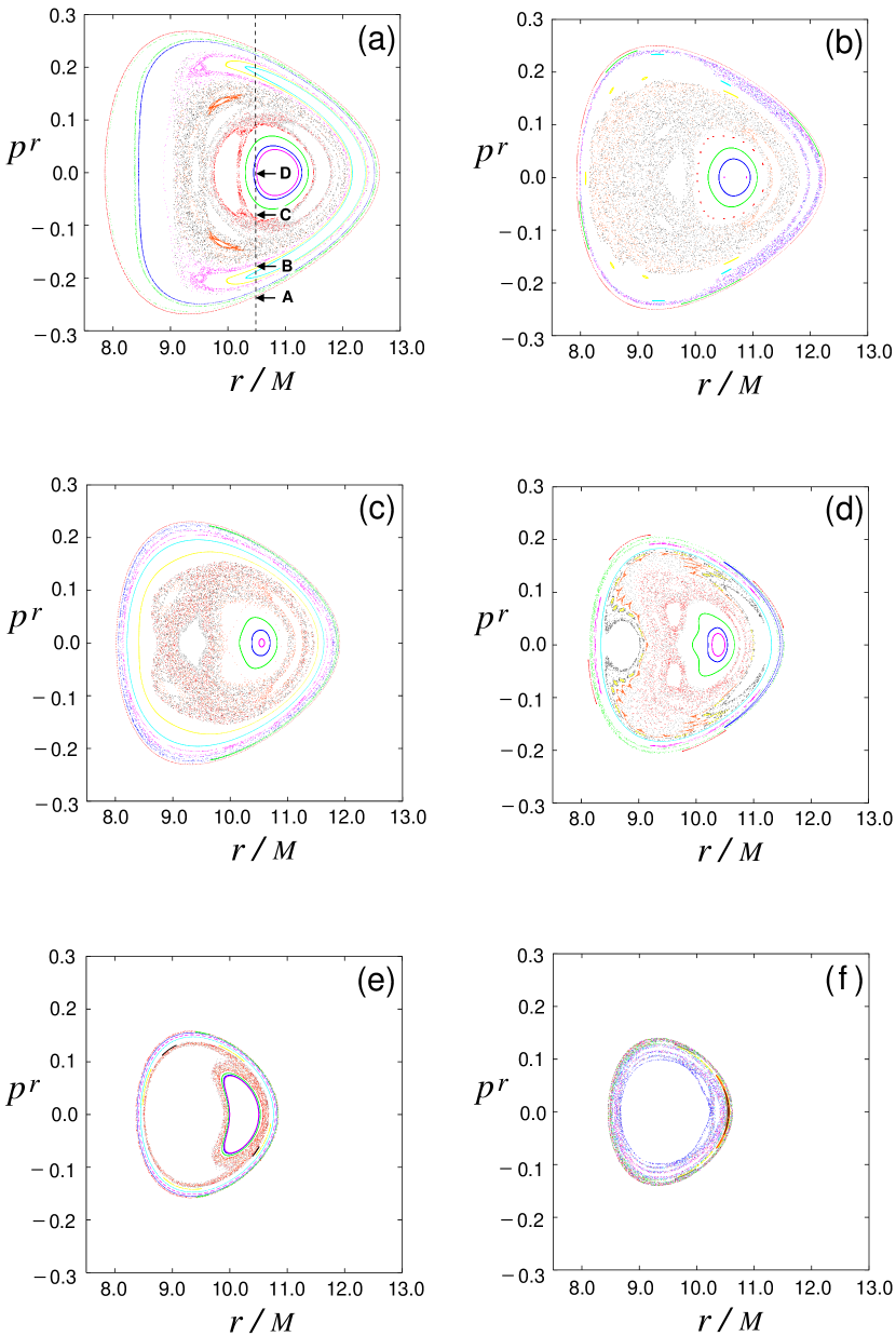
Figure 9: The Poincaré map of a charged particle orbiting in the dipole magnetic field around a black hole of $a=0.9M$. The parameters for the motion are (a) $E/m=0.900$, (b) $E/m=0.895$, (c) $E/m=0.890$, (d) $E/m=0.885$, (e) $E/m=0.875$ and (f) $E/m=0.872$ with $L/m=-7.0M$, $Q_{d}=70.0M^{2}$, $r_{\rm ini}=10.5M$ and $\theta_{\rm ini}=\pi/2$.

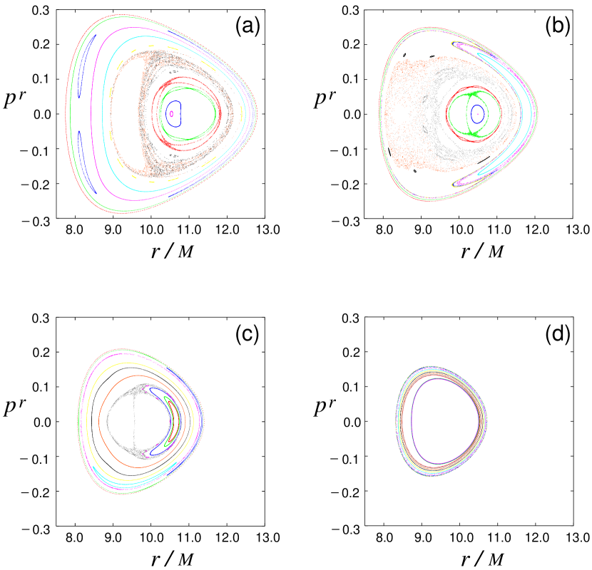
Figure 10: The Poincaré map of a charged particle orbiting in the dipole magnetic field around a black hole of $a=M$. The parameters for the motion are (a) $E/m=0.900$, (b) $E/m=0.890$, (c) $E/m=0.880$ and (d) $E/m=0.870$ with $L/m=-7.0M$, $Q_{d}=70.0M^{2}$, $r_{\rm ini}=10.5M$ and $\theta_{\rm ini}=\pi/2$.

Figures 7–10 show several typical examples of the Poincaré map for various hole’s spin and particle’s energies. We find the spin effects on the trajectories in the Poincaré map. For slowly rotating black hole cases, the region of random trajectories fill a finite portion of the energy surface in phase space; see Fig. 7. The intersections of a single random trajectory with the surface of section fill a finite area. For a rotating black hole cases, both types of trajectories are mixed; see Figs. 8 and 9. That is, the distribution on the Poincaré map makes wide rings by random trajectories, and closed curves by regular trajectories. These differences on their trajectories depend on the initial ejection angle $\psi_{\rm ini}$. Specially, for rapidly rotating black hole cases, the ratio of the regular orbits increases rather than mildly rotating black hole case; see Fig. 9. The hole’s spin effects weaken the chaotic motion in the black hole magnetosphere. In fact, for the maximally rotating black hole case, for a wide range of $\psi_{\rm ini}$-values the regular orbits are observed, although random trajectories also appear for larger energy particle motions; see Fig. 10.

Next, let us see the energy dependences on the Poincaré map. For a slowly rotating black hole case (see Fig. 7), the random nature of intersections on the Poincaré map is almost independent of particle’s energy. The outer boundary of cross sections plotted by the trajectory of $p_{\theta}^{\rm ini}=0$ only shrinks with decreasing the particle’s energy; it depends on the effective potential well specified by the values of $Q_{d}$, $L$ and $a$ (Karas & Vokrouhlick’y, 1992). We also see a few void regions on the map in some cases. On the other hand, we find the energy dependence of the Poincaré map for mildly and rapidly rotating black hole cases. In Figures 8a and 8c (where $a=0.6M$), most trajectories are chaotic, but in Figures 8b and 8d the regular trajectories appear on the map (less chaotic). Figure 9 and 10 show the cases of rapidly rotating black hole case. The regular trajectory is obtained when the elevation of the particle ejected is small (somewhat parallel to the equator) or large (somewhat perpendicular to the equator), while the random trajectory is observed when the elevation has an intermediate value of them. For example, in Figure 9a, when the initial value of $p^{r}$ is in the range of A–B or C–D, the regular trajectories are obtained, while the range of B–C shows random trajectories.

Although the charged particle is trapped in the effective potential well, when the energy has an almost minimum value at the injection point; that is, $E/m\sim V_{\rm eff}(r_{\rm ini},\theta_{\rm ini})$, the intersections of the whole trajectories are bounded by outer and inner closed curves, which make a narrow layer; see Figs. 9f and 9d. The inner boundary of the cross section is plotted for the orbit of $p^{r}_{\rm ini}=0$. Note that, in the case of $a\gtrsim 0.6M$, some orbits with their almost minimum energy show the random trajectories on the Poincaré map, but the region of the random trajectories is restricted within a narrow torus-like belt. The width of this belt becomes narrow when the particle’s energy has its minimum energy that is specified as the value of the effective potential at the particle’s injected point; for a slowly rotating black hole case, such a belt-like distribution does not appear on the map. In summary, we see the tendency that random trajectories are independent of the initial injection angles and their energy in a slowly rotating black hole spacetime. For a rapidly rotating black hole case, however, we also see regular trajectories, which depend on the initial injected angle and also their energy.

5 Discussion

In § 2, we have mentioned that in a stationary and axisymmetric black hole magnetosphere there are only three constants of motion, $\pi_{t}=E$, $\pi_{\phi}=-L$ and $m$, and as a consequence of the non-existence of the forth integral of motion, $\pi_{\theta}$, the chaos would appear in the system. In spite of being a non-integrable system, however, we have found the regular trajectories on the Poincaré map, although we have also seen the chaotic trajectories (for the different injection angles). In this section, we discuss the reason.

As shown in Figures 4–6, a particle in the black hole dipole magnetic field is trapped when a black hole rotates. It bounces back and forth between the northern and southern mirrors (also called magnetic bottle). Since the regular or random trajectories depend discontinuously on a choice of initial angle, their presence does not imply the existence of a global invariant of the system. However, if regular trajectories exist, they should represent some kind of invariants of the motion. These trajectories are conditionally periodic with angle variables. With this motion an adiabatic invariant would be associated, and that is related to the longitudinal motion. Then, we define the action integral as (see, e.g., Goedbloed & Poedts, 2004)

$$J_{\theta}\equiv\frac{1}{\ell}\oint\ \sqrt{-p_{\theta}p^{\theta}}\ d\lambda\ ,$$ (13)

where the integral is taken over one cycle of the oscillation in time and $\ell$ is the length of one cycle of the path. In general, the value of $J_{\theta}$ is not a constant for each cycle of the oscillation of a test-charge in the black hole dipole magnetic field around a central object, so that we will see random trajectories (chaos). In fact, for a slowly rotating black hole, we see that most orbits with the various injection angles are chaotic, and their $J_{\theta}$-values are not constants; they vary irregularly. However, we can also observe the regular trajectories, when the action integral of $J_{\theta}$ is nearly constant for a long-time orbital motion. For a rotating black hole case, we can find the regular trajectory where the value of $J_{\theta}$ becomes approximately constant, while it oscillates slightly in a few cycles. Note that the “Carter’s constant ${\cal Q}$” fluctuates in time; that is, the value of ${\cal Q}$ defined by equation (6) is not a constant. In this case, the motion shows a regular trajectory on the Poincaré map. Thus, we find that the motion of a test charge in the magnetosphere around a rotating black hole can be nearly integrable.

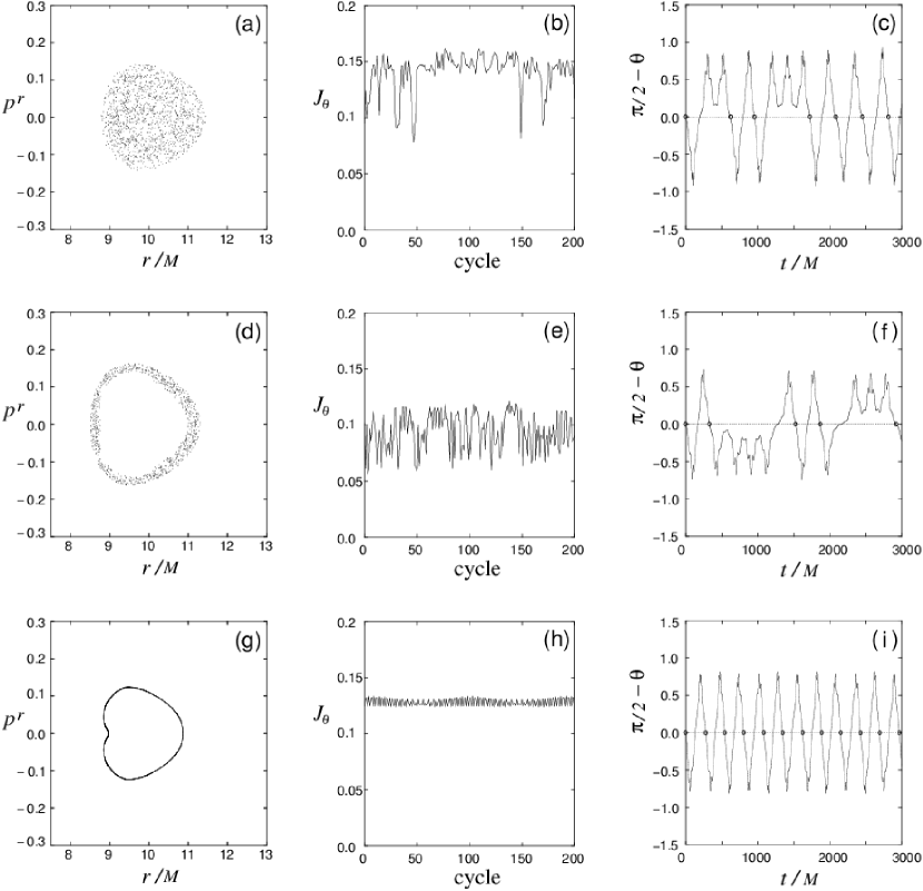
Figure 11: Various types of the Poincare map (LEFT column). Many points on the Poincare maps (a, d) are plotted by stochasticity (chaos), while that on the Poincare map (g) shows regular trajectory. The action integral $J_{\theta}$ (CENTER column) and the time series of $\pi/2-\theta$ (RIGHT column), where the first several cycles are shown, are also presented. Small circles in the time series correspond to the points plotted on the Poincaré map. The values of $J_{\theta}$ are almost constant for (h) regular trajectories. The parameters of these trajectories are set as (a, b, c) $a=0.3M$, $E/m=0.900$, $\psi_{\rm ini}=-0.10\pi$, (d, e, f) $a=0.6M$, $E/m=0.890$, $\psi_{\rm ini}=-0.10\pi$, (g, h, i) $a=0.6M$, $E/m=0.890$, $\psi_{\rm ini}=-0.30\pi$. The remaining parameters are $L/m=-7.0M$, $Q_{d}=70.0M^{2}$, $r_{\rm ini}=10.5M$ and $\theta_{\rm ini}=\pi/2$.

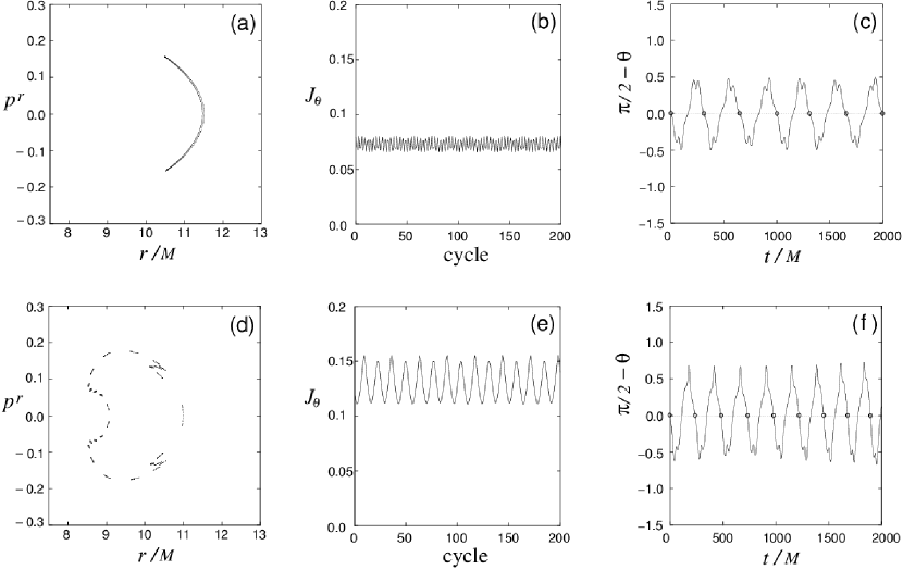
Figure 12: Examples of the Poincare map (LEFT column) for $a=0.9M$ case. The regular trajectories are shown. The action integral $J_{\theta}$ (CENTER column) and the time series of $\pi/2-\theta$ (RIGHT column), where the first several cycles are shown, are also presented. The parameters of these trajectories are set as (a, b, c) $\psi_{\rm ini}=-0.10\pi$ and (d, e, f) $\psi_{\rm ini}=-0.22\pi$. The other parameters are $E/m=0.885$, $L/m=-7.0M$, $Q_{d}=70.0M^{2}$, $r_{\rm ini}=10.5M$ and $\theta_{\rm ini}=\pi/2$.

The region of random trajectories fill a finite portion of the surface of a section in phase space. Figure 11a shows that the typical intersections of a single random trajectory with the surface of a section fill a finite area, where the value of $J_{\theta}$ varies irregularly; see Fig. 11b. The time series of $\pi/2-\theta$ also shows an irregular feature in Fig. 11c. In Figure 11d, we see an annular layer randomly filled with intersections of a single trajectory lying between two invariant curves. We also see periodic trajectories that are composed by small regular trajectories inside these randomly filled regions (see, e.g., Figs. 8d and 9d). Such a structure may be related to resonances of the orbits that play a crucial role in the appearance of random motions in near-integrable systems (Lichtenberg & Liberman, 1992). In this paper, however, we do not discuss about the details. In this annular layer case, we also see that the value of $J_{\theta}$ varies irregularly; see Fig. 11e. On the other hand, in Figure 11g, we see a generic trajectory that covers the surface of the torus. The motion along the dipole magnetic field line is almost periodic in the $\theta$-direction; see Fig. 11i. The intersections of the trajectory with the surface of a section at a value of $\psi_{\rm inj}$ lie on a closed invariant curve and densely cover the curve over long periods of time. The value of $J_{\theta}$ is nearly constant as shown in Figure 11h. Figure 12 shows the other characteristic trajectories in a rotating black hole spacetime; see also Fig. 6. In Figure 12(TOP), the crescent regular trajectory is presented, where the value of $J_{\theta}$ is approximately constant. On the other hand, in Figure 12(BOTTOM), many islands of a trajectory distribute on a curve. This shows a regular trajectory. However, the value of $J_{\theta}$ is not a constant, and it oscillates periodically. When we consider the average of $J_{\theta}$ during dozens of cycles of oscillations, the value is almost constant over long periods of cycles. It seems that this feature is enough to guarantee the generation of the regular trajectory.

The ratio of the regular trajectories on the Poincaré map increases with the value of the hole’s spin. Specially, for the maximally rotating case of $a=M$, almost trajectories become regular; see Fig. 10. It seems that the fourth constant of motion is generated for the system with the black hole dipole magnetic field in the $a\to M$ limit. One may expect that, by using the dipole magnetic fields (9) and (10), the equation of motion can be separable with respect to the $r$ and $\theta$ coordinates, and the “modified Carter constant” including the magnetic field terms may be redefined. However, without the separable treatment on the basic equation, we find the constancy of $J_{\theta}$ in this system numerically. Exactly speaking, for the regular trajectories appeared in this system the value of $J_{\theta}$ is not necessary to be a constant; in fact it oscillates periodically. However, for a regular trajectory, we can regard the value of $J_{\theta}$ (or the average on a few cycles) as a constant approximately, comparing with that of chaotic trajectories. Even in the $a\to M$ limit, this constancy can be broken depending on the injection angle. In fact, for larger $E/m$, we can also see an annular layer of randomly filled by trajectories.

Our result suggests that the saddle in the double-well potential plays an important role for chaotic motions of a charged particle. Similar behavior has been investigated in Hamiltonian dynamical systems (Reichl & Zheng, 1984). In the limit of $a\to M$, however, we see that the feature of the double well potential vanishes. Then, the chaotic behavior weakens, where many regular trajectories are observed. The property of chaos and/or regular trajectories in the dipole magnetic field around a rapidly rotating black hole is related to the hole’s spin dependence on the effective potential, which is generated by the combination of the electromagnetic force, the gravitational force and the centrifugal force. Although in this paper we consider the black hole dipole magnetic field, we could understand the basic properties of a charged particle by considering the distribution of the effective potential when we treat a motion of a test charge in any arbitrary electromagnetic field around a black hole. It is a future work to confirm the above suggestion by more detailed analysis.

6 Concluding Remarks

In this paper, we have discussed the off-equatorial motion of a test charge in the black hole dipole magnetosphere. The charged particle gyrates around a magnetic field line, drifts in the toroidal direction and oscillates between the northern and southern hemisphere, and then the orbits becomes very complicated. So, the numerical study by the Poincaré map is effective. Then, we find the spin dependence of the trajectory on the Poincaré map. That is, for a slowly rotating black hole case, the particle’s trajectory shows chaos. More interestingly, we also find that, for a rapidly rotating black hole case, the chaotic behavior of the trajectories weakens and the fourth invariance of the motion, which is an adiabatic invariant related to the longitudinal motion, can be approximately generated.

The chaotic motion in a black hole magnetosphere may be related to the origin of cosmic rays. The magnetic mirror concepts play a prominent role in space and plasma astrophysics. Examples are the Van Allen belt in the magnetosphere of the Earth, where high energy particles are trapped in a magnetic bottle and some kind of acceleration mechanisms are expected. In the case of a black hole magnetosphere, we may expect the formation of the magnetic bottle near the black hole. When such a situation is realized, the particles trapped in the “black hole Van Allen belt” would emit high-energy radiation, or some particles may accelerate to ultra-relativistic velocity by some electromagnetic interactions (ex., the Fermi acceleration by the perturbed magnetic bottle). Furthermore, some kinds of waves (i.e., Alfvén waves and/or fast waves) in the magnetosphere will give influence to the motion of a particle moving in a magnetized plasma. Our simple model with the black hole dipole magnetic field presented here could be a preliminary step toward the understanding the motion of charged particles around a black hole.

In this paper, we do not consider the interactions between charged particles, and the emission process from the chaotic/regular motion of a charged particle. However, we can expect that the spectrum emitted from such charged particles in periodic motions in the inhomogeneous magnetic field carries the informations on the black hole spin and the strength and/or distribution of the electromagnetic field. These studies should be considered in future works.

References

- Aliev & Özdemir (2002) Aliev, A. N., & Özdemir, N. 2002, MNRAS, 336, 241
- Blandford & Znajek (1977) R. D. Blandford, & R. L. Znajek, MNRAS, 179, 433 (1977)
- Camenzind (1987) Camenzind, M. 1987, A&A, 184, 341
- Chitre & Vishveshwara (1975) Chitre, D. M., & Vishveshwara, C. V. 1975, Phys. Rev. D, 12, 1528
- Esteban & Medina (1990) Esteban, E. P., & Medina, I. R. 1990, Phys. Rev. D, 42, 307
- Ghosh (2000) Ghosh, P. 2000, MNRAS, 315, 89
- Goedbloed & Poedts (2004) Goedbloed, J. P. H., & Poedts, S. 2004, Principles of Magnetohydrodynamics (Cambridge, Cambridge Univ. Press)
- Karas & Vokrouhlick’y (1992) Karas, V., & Vokrouhlick’y, D. 1992, Gen. Rela. Grav., 24, 729
- Koyama, Kiuchi & Konishi (2007) Koyama, H., Kiuchi, K., & Konishi, T. 2007, Phys. Rev. D, 76, 064031
- Li (2000) Li, L.-X. 2000, Phys. Rev. D, 61, 084016
- Lichtenberg & Liberman (1992) Lichtenberg, A. J., & Liberman, I. A. 1992, Regular and Chaotic Dynamics second edition (New York, Springer)
- Misner, Thorne & Wheeler (1973) Misner, C. W., Thorne, K. S., & Wheeler, J. H. 1973, Gravitation (San Francisco, Freeman), chap 33
- Nakamura & Ishizuka (1993) Nakamura, Y., & Ishizuka, T. 1993, Astrophys. & Space Sci., 210, 105
- Nitta, Takahashi, & Tomimatsu (1991) S. Nitta, M. Takahashi, & A. Tomimatsu, Phys. Rev., D44, 2295 (1991)
- Petterson (1975) Petterson, J. A. 1975, Phys. Rev. D, 12, 2218 Prasanna, A. R. 1975, Pramana, 8, 229
- Prasanna (1978) Prasanna, A. R. 1978, Bullutin of the Astrophysical Society of India, 6, 88
- Prasanna (1980) Prasanna, A. R. 1980, Riv. Nuovo Cimento, 3, N., 11, 1
- Rees (1998) Rees, M. J. 1998, in Wald, R.D. ed., Black Holes and Relativistic Stars (Chicago, Chicago Univ. Press)
- Reichl & Zheng (1984) Reichl, L. E., & Zheng, W. M. 1984, Phys. Rev. A, 29, 2186
- Tomimatsu & Takahashi (2001) Tomimatsu, A., & Takahashi, M., 2001, ApJ, 552, 710