Hot-spot model for accretion disc variability as random process

Abstract

Aims. Theory of random processes provides an attractive mathematical tool to describe the fluctuating signal from accreting sources, such as active galactic nuclei and Galactic black holes observed in X-rays. These objects exhibit featureless variability on different timescales, probably originating from an accretion disc.

Methods. We study the basic features of the power spectra in terms of a general framework, which permits semi-analytical determination of the power spectral density (PSD) of the resulting light curve. We consider the expected signal generated by an ensemble of spots randomly created on the accretion disc surface. Spot generation is governed by Poisson or by Hawkes processes. The latter one represents an avalanche mechanism and seems to be suggested by the observed form of the power spectrum. We include general relativity effects shaping the signal on its propagation to a distant observer.

Results. We analyse the PSD of a spotted disc light curve and show the accuracy of our semi-analytical approach by comparing the obtained PSD with the results of Monte Carlo simulations. The asymptotic slopes of PSD are $0$ at low frequencies and they drop to $-2$ at high frequencies, usually with a single frequency break. More complex two-peak solutions also occur. The amplitude of the peaks and their frequency difference depend on the inherent timescales of the model, i.e., the intrinsic lifetime of the spots and the typical duration of avalanches.

Conclusions. At intermediate frequencies, the intrinsic PSD is influenced by the individual light curve profile as well as by the type of the underlying process. However, even in cases when two Lorentzians seem to dominate the PSD, it does not necessarily imply that two single oscillation mechanisms operate simultaneously. Instead, it may well be the manifestation of the avalanche mechanism. The main advantage of our approach is an insight in the model functioning and the fast evaluation of the PSD.

1 Introduction

It is widely accepted that massive black holes with accretion discs reside in cores of active galactic nuclei, where most activity originates and X-rays are produced (e.g., Blandford et al. 1990). The observed light curves, $f\,\equiv\,f(t)$, show irregular, featureless fluctuations with a very complex behaviour, practically at every studied frequency (Gaskell et al. 2006). Variability has been traditionally analysed by the Fourier method (Feigelson & Babu 1992). Remarkably, a number of similarities appear between the properties of massive black holes in galactic nuclei and those in X-ray binaries, suggesting that some kind of universal rescaling operates according to central masses of these systems (Mirabel & Rodríguez 1998). This concerns also the X-ray power spectra (e.g., Markowitz et al. 2003; McHardy et al. 2006).

Light curves can be characterised by an appropriate estimator of the source variability which, in the mathematical sense, is a functional: $f\rightarrow\mathcal{S}\left[f\right]$. We accept the idea that the signal resulting from a spotted accretion disc is intrinsically stochastic, likely originating from turbulence. Hence, $\mathcal{S}\left[f\right]$ is a random value. It can be a number (for example, the ‘rms’ characteristic), function of a single variable (for example, the power-spectral density – PSD) or of many variables (e.g., poly-spectra, rms–flux relation, etc). The appropriate choice depends on the type of information we seek and the quality of data available. The PSD is a traditional and widely utilised method to examine variable signals, and the AGN light curves are no exception. A typical signal can be represented by a broad band PSD with the tendency towards flattening at low frequency (Lawrence et al. 1987; McHardy & Czerny 1987; Lawrence & Papadakis 1993; Mushotzky et al. 1993; Uttley et al. 2002).

There is an ongoing debate about the overall shape of the PSD and the occurrence of the break frequency or, possibly, two break frequencies at which the slope of the PSD can change (Nowak et al. 1999; Markowitz et al. 2003). In the case of a widely-studied Seyfert galaxy, MCG–6-30-15, McHardy et al. (2005) have closely examined the slope of PSD, namely its bending, with RXTE and XMM-Newton data. It is worth noticing that the accurate fits to the X-ray sources seem to exhibit a multi-Lorentzian structure rather than a simple power law. The same is true for the best studied example, the Seyfert 1 galaxy Akn 564 (McHardy et al. 2007).

It was proposed (Abramowicz et al. 1991; Zhang & Bao 1991; Wiita et al. 1992) that hot spots contribute to the variability of the AGN variability, or that they could even be the dominant process shaping the variability pattern. These spots should occur on the disc surface following its intermittent irradiation by localised coronal flares (Galeev et al. 1979; Merloni & Fabian 2001; Czerny et al. 2004). Here, the “spots” represent a somewhat generic designation for non-axisymmetric features evolving on the disc surface in connection with flares. They share the bulk orbital motion with the underlying disc. The observed signal is thus modulated by relativistic effects as photons propagate towards a distant observer.

Various schemes have been discussed in which the fluctuations of the disc emissivity at different points of space and time are mutually interconnected in some way. In particular, the avalanche model (Poutanen & Fabian 1999; Życki 2002; Życki & Niedźwiecki 2005) seems to be physically substantiated within the framework of magnetically-triggered flares and spots. It is also a promising model capable to reproduce, for example, the broken power-law PSD profiles. Notice, however, that other promising ideas were proposed (e.g., Mineshige et al. 1994; Lyubarskii 1997), provoking the question of whether a common mathematical basis could reflect the entire range of models and provide us with general constraints, independent of (largely unknown) model details.

We add to this model by applying the method of random point processes (Cox & Miller 1965). Interestingly enough, a rather formal approach can provide useful analytical formulae defining the basic form of the expected power spectrum. Apart from this practical aspect, we suggest that the concept discussed here offers much better insight into various influences that shape the expected form the power spectrum. These are very attractive features especially with respect to avalanche models, which may have different flavours, typically with a vast parameter space, thus proving very demanding to examine in a systematic manner.

Even more important is that the adopted formalism provides a very general tool and allows for a broader perspective on different mechanisms of variability (Pecháček & Karas 2007). We develop the idea in a systematic way and give the explicit correspondence between our approach and some of the above-mentioned and widely-known scenarios (Abramowicz et al. 1991; Poutanen & Fabian 1999). This description provides semi-analytical solutions, convenient to search through a broad parameter space. Our results can help to identify how the intrinsic properties of individual flares and the relativistic effects influence the overall PSD. In particular, we can identify those situations in which a doubly-broken power law occurs.

We consider stochastic processes (e.g., Feller 1971; Gardiner 1994) in the framework appropriate for modelling the accretion disc variability. In particular, in Sect. 2 we consider a simple model of a spotted accretion disc constrained by the following three assumptions about the creation and evolution of spots: (i) each spot is described by its time and place of birth ($t_{j}$, $r_{j}$ and $\phi_{j}$) in the plain of the disc; (ii) every new occurrence starts instantaneously; afterwards, the emissivity decays gradually to zero (the total radiated energy is of course finite); and (iii) the intrinsic emissivity is fully determined by a finite set of parameters which form a vector, $\mbox{\boldmath$\xi$}_{j}$, defining the light curve profile. Later on, we will consider the modulation of the intrinsic emission by the orbital motion and relativistic lensing. The disc itself has a passive role in our considerations; we will treat it as a geometrically thin, optically thick layer lying in the equatorial plane.

Because of the apparently random nature of the variability, we adopt a stochastic model in which the creation of spots is governed by a random process. The assumption that spots are mutually statistically independent seems to be a reasonable (first) approximation, however, we find that we do need to introduce some kind of relationship between them. This connection is discussed in Sect. 3. The statistical dependence among spots can be introduced in several ways. In Sect. 4, we explore in detail the specific models of interrelated spots using the formalism of Hawkes-type processes. Conclusions are summarised in Sect. 5. Finally, in the Appendix we provide some mathematical prerequisites, which the reader may find useful to understand the general background of the paper, and we also summarise the mathematical notation.

2 Models of stochastic variability

2.1 Orbiting spots and relativistic effects

We will apply our investigations to models where the signal is produced by point-like orbiting spots (circular Keplerian motion along the azimuthal $\phi$ direction). The intrinsic emission, produced in the local co-orbiting frame of the spot, is influenced by the Doppler effect and gravitational lensing, which cannot be ignored at typical distances of several units or tens of gravitational radii. Photons emitted at different moments and positions experience different light-travel time on the way towards the observer, so the observed timing properties should reflect this specific modulation. We adopt the Schwarzschild metric for the gravitational field and employ the method of transfer function (Pecháček et al. 2005, 2006) to describe the light amplification (or dilution); $\theta_{\rm o}$ is inclination angle of the observer ($\theta_{\rm o}=90$ deg corresponds the edge-on view of the disc plane). The periodical modulation of the observed signal is included in the transfer function $F(t,r,\theta_{\rm o})\equiv F(\phi(t),r,\theta_{\rm o})$. An implicit relation holds for the phase,

$$\phi(t)=\Omega t-\delta t(\phi(t),r,\theta_{\rm o}),$$ (1)

where the effect of time delays $\delta t(\phi,r,\theta_{\rm o})$ is taken into account. The modulation by $F$ is superimposed onto that due to intrinsic timescales present in the signal from spots. Then, for the final flux $f(t)$ measured by a distant observer, we write $f(t)=IF(t,r,\theta_{\rm o})$.

In the case of an infinitesimal surface element with intrinsically constant and isotropic emissivity $I$, orbiting with Keplerian orbital frequency $\Omega(r)$, the flux measured by a distant observer varies just as $F$ changes along the orbit.

We remind the reader that the mass of central black holes in galactic nuclei is in the range of $\simeq M\approx 10^{6}$–$10^{9}\,M_{\odot}.$ Mass of the accretion disc is at least three orders of magnitude smaller than the black hole mass, so we neglect it in our calculations (the accretion disc self-gravity may be important for its intrinsic structure, but the direct gravitational effect on light is quite small; Karas et al. 1995). Hence, the gravitational field can indeed be described by a vacuum black-hole spacetime (Misner et al. 1973). We use geometrical units with $c=G=1$. Transformation to physical scales can be achieved when the mass of the central black hole is specified because Keplerian frequency scales inversely with the gravitational radius. The gravitational radius of a massive black hole is $R_{\rm g}\equiv c^{-2}GM\approx 0.48\times 10^{-5}M_{8}\,$pc, and the corresponding characteristic time-scale is $t_{\rm g}\equiv c^{-3}GM\approx 0.49\times 10^{3}M_{8}\,$sec, where the mass $M_{8}\equiv M/(10^{8}M_{\odot})$. All lengths and times can be made dimensionless by expressing them in units of $M$, so they can be easily scaled to different masses. For example, for the Keplerian orbital period we obtain $T_{\rm{}orb}\approx 3.1\times 10^{3}\,r^{3/2}M_{8}$, where the radius is expressed in units of $R_{\rm g}$ and $T_{\rm orb}$ is given in seconds.

Let us note that the intrinsic timescales of the spot evolution and of avalanches (both timescales will be discussed below) need not to be directly connected with the Keplerian orbital period. This internal freedom of the model can help to bring the predicted frequency of the breaks of the PSD profile in agreement with the data.

2.2 Model driven by a general point process

Now we will describe the process of the creation of spots from the statistics point of view. Let us consider a signal of the form

$$f(t)=\sum\limits_{j}I(t-{\delta_{j}},\,\mbox{\boldmath$\xi$}_{j})\,F(t-\delta_{{\rm p}j},r_{j}).$$ (2)

The underlying process consists of a sequence of events which, in general, can be either mutually independent, or there can be some statistical dependence among them. Naturally, the latter case will be more complicated and interesting. In Eq. (2), $I(t,\,\mbox{\boldmath$\xi$})=g(t,\,\mbox{\boldmath$\xi$})\,\theta(t)$ is the light curve profile of a single event; $\delta_{j}=t_{j}+t_{{\rm d}j}$ and $\delta_{{\rm p}j}=\delta_{j}+t_{{\rm p}j}$ are the time offsets (determined by the moment of the ignition of the spot) and the initial time delay (which is an arbitrary but fixed value); $\theta(t)$ is the Heaviside function; and $g(t,\mbox{\boldmath$\xi$})$ is a non-negative function of $k+1$ variables, $t$ and $\mbox{\boldmath$\xi$}=(\xi^{1},\dots,\xi^{k})$. Hereafter, we omit the explicit dependency on $\theta_{\rm o}$.

Figure 1: Illustrating the correspondence between the ignition moments of the elementary events and the resulting light curve. The model is fully determined by a set of points in ($t$–$\tau$) plane, representing the pairs of ignition time $t$ versus the time constant $\tau$ of each event (panel a), and the elementary light curves with the profile $I(t,\tau)=\left(t/\tau\right)^{2}\exp\left(-t/\tau\right)\theta(t)$ (panel b). The total light curve (panel c) is represented as a sum of the individual contributions.

Quantities $\mbox{\boldmath$\xi$}_{j}$, $t_{j}$, $r_{j}$, $t_{{\rm p}j}$ and $t_{{\rm d}j}$ are random values. The vector $\mbox{\boldmath$\xi$}_{j}$ determines the duration and shape of each event ($t_{j}$ is time of ignition; parameter $t_{{\rm p}j}$ determines the initial phase of the periodical modulation of the $j$–th event; and $t_{{\rm d}j}$ is the corresponding initial time-offset). These assumptions bring the formulation of the problem close to the framework studied by Brémaud et al. (2002; 2005). We will calculate the power spectrum of this process directly from Eq. (100) in the Appendix.

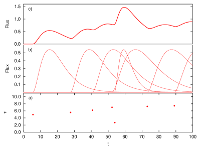
We remark that for the amplitudes of individual events we assume the identical values (at each given radius). This restriction is imposed only for the sake of definiteness of our examples; the formalism can deal with a distribution of amplitudes. Indeed, we do not impose any serious constraint on the model because the information about the level of the fluctuating signal can be adjusted by setting the frequency of the events (Lehto 1989). A simple demonstration of this concept is shown in Fig. 1. This plot illustrates how the model light curve arises from the elementary components. Naturally, we can approach such decomposition from another angle, by investigating how the total light curve can be expressed in terms of some basic profile. It is important to realise that, for the purposes of our present paper, light curves are of secondary importance. Instead, our calculations allow us to proceed from the distribution of the onset times and the characteristics of individual flares directly to the power spectral density, which stands as the primary characteristic of the source signal.

Equation (2) represents a very general class of random processes. By applying the Fourier transform, we find

$$\mathcal{F}_{T}\big{[}f(t)\big{]}(\omega) = \frac{2\sin(T\omega)}{\omega}\;\star\;\sum\limits_{j}\mathcal{F}\big{[}I(t-{\delta_{j}},\,\mbox{\boldmath$\xi$}_{j})$$ (3)

$$\times\;F(t-\delta_{{\rm p}j},r_{j})\big{]}(\omega),$$

where $\star$ denotes the convolution operation. In Eq. (2), we sum together a set of all events (this infinite sum could in general pose problems with convergence, however, as we will see later, we can restrict the sum to a finite set of events without any loss of generality). The Fourier transform of a single event, $I(t-{\delta_{j}},\,\mbox{\boldmath$\xi$}_{j})F(t-\delta_{{\rm p}j},\,r_{j})$, is then

$$\mathcal{F}\big{[}I(t-{\delta_{j}},\,\mbox{\boldmath$\xi$}_{j})F(t-\delta_{{\rm p}j},r_{j})\big{]}(\omega)$$

$$\quad=e^{-i\omega\delta_{j}}\mathcal{F}\big{[}I(t,\mbox{\boldmath$\xi$}_{j})\big{]}\star\mathcal{F}\big{[}F(t+t_{{\rm p}j},r_{j})\big{]}(\omega).$$ (4)

Periodical function $F(t,r)$ can be now expanded in a series, $F(t,r)=(2\pi)^{-1}\sum\limits c_{k}(r)\exp[{ik\Omega(r)t}]$, and the expanded form substituted in the incomplete Fourier transform of $f(t)$.

Knowing the incomplete Fourier transform of $f(t)$, we can calculate its squared absolute value and perform the averaging over all realisations of the process. This can be simplified by assuming that every single event quickly decays. In principle, between $-T$ and $T$ the process is influenced by all events ignited during the whole interval $\langle-\infty,T\rangle$, however, because of the fast decay of the events, the interval can be restricted to $\langle-(T+C),T\rangle$, where $C$ is a sufficiently large positive constant. In other words, every realisation of the process $f(t)$ on $\langle-T,T\rangle$ can be described by a set of points in $(k+4)$-dimensional space $(t_{j},t_{{\rm d}j},t_{{\rm p}j},r_{j},\mbox{\boldmath$\xi$}_{j})$ with $-(T+C)\leq t_{j}\leq T$.

Values of the initial time delay and phase are functions of initial position of each spot, i.e.

$$t_{{\rm d}j}=\delta t(r_{j},\phi_{j}),\qquad t_{{\rm p}j}=\frac{\phi_{j}}{\Omega(r_{j})}+t_{{\rm d}j}.$$ (5)

Fourier transform of the resulting signal is then

$$\mathcal{F}\big{[}I(t-t_{{\rm d}j},\,\mbox{\boldmath$\xi$}_{j})\,F(t-t_{{\rm d}j}+t_{{\rm p}j},r_{j})\big{]}(\omega)=\sum\limits_{k=-\infty}^{\infty}c_{k}(r)\,e^{ik\phi}\,\mathcal{F}_{k},$$ (6)

where $\mathcal{F}_{k}\equiv\mathcal{F}[I(t-\delta t(r,\phi),\mbox{\boldmath$\xi$})](\omega-k\Omega(r))$ is the Fourier transform of the event light curve, corrected for the time delay. Every realisation of this process is completely determined by the set of points $(t_{j},\phi_{j},r_{j},\mbox{\boldmath$\xi$}_{j})$.

Defining the function

$$s(t,\phi,r,\mbox{\boldmath$\xi$};\omega) = \frac{2\sin(T\omega)}{\omega}\star\Big{(}e^{-i\omega t}\!\sum\limits_{k=-\infty}^{\infty}\!c_{k}(r)e^{ik\phi}$$ (7)

$$\times\mathcal{F}\left[I(t-\delta t,\,\mbox{\boldmath$\xi$})\right](\omega-k\Omega(r))\Big{)}$$

we can write

$$\big{|}\mathcal{F}_{T}[f(t)](\omega)\big{|}^{2}=\Big{|}\sum\limits_{j}s(t_{j},\,\phi_{j},\,r_{j},\,\mbox{\boldmath$\xi$}_{j};\,\omega)\Big{|}^{2}.$$ (8)

Due to Campbell’s theorem (105),

$$\!\!\!{\rm E}\left[\left|\mathcal{F}_{T}[f(t)](\omega)\right|^{2}\right]=\int\limits_{A\times A^{\prime}}s(t,\phi,r,\mbox{\boldmath$\xi$};\omega)$$

$$\!\times\,s^{*}(t^{\prime},\phi^{\prime},r^{\prime},\mbox{\boldmath$\xi$}^{\prime};\omega)\,m_{2}(t,\phi,r,\mbox{\boldmath$\xi$},t^{\prime},\phi^{\prime},r^{\prime},\mbox{\boldmath$\xi$}^{\prime})\,{\rm d}A\,{\rm d}A^{\prime},$$ (9)

where $m_{2}$ is density of the second-order moment measure $M_{2}(.)$ corresponding to the random point process of $(t_{j},\phi_{j},r_{j},\mbox{\boldmath$\xi$}_{j})$, $A$ is a Cartesian product of four sets representing the domains of definitions, i.e.

$$A=\langle-(T+C),T\rangle\times\langle 0,2\pi\rangle\times\langle r_{\rm min},r_{\rm max}\rangle\times\Xi.$$ (10)

Now we can perform the limit of $T\rightarrow\infty$, as given by Eq. (100) in the Appendix. It can be shown that the result is independent of the value of $C$. Therefore, to obtain an explicit formula for the PSD we need only to specify the form of $m_{2}(.)$ in Eq. (9). Hereafter, we will show how to proceed with this task.

2.3 Model driven by the Poisson process

To start with a simple example, we assume mutually independent events with uniformly distributed ignition times. In other words, in this subsection we assume that there is no relationship among different spots – neither in their position nor in the time of birth (spots are statistically-independent). The intensity and the second-order measure are

$$M_{{\rm g}1}({\rm d}t) = \lambda\,{\rm d}t,$$ (11)

$$M_{{\rm g}2}({\rm d}t\,{\rm d}t^{\prime}) = \left[\lambda^{2}+\lambda\delta(t-t^{\prime})\right]{\rm d}t\,{\rm d}t^{\prime},$$ (12)

where $\lambda$ is the mean rate of events. Other parameters are treated as independent marks with common distribution $G({\rm d}\phi\,{\rm d}r\,{\rm d}\mbox{\boldmath$\xi$})$. The second-order measure is

$$\!\!\!M_{2}({\rm d}t\,{\rm d}\phi\,{\rm d}r\,{\rm d}\mbox{\boldmath$\xi$}\,{\rm d}t^{\prime}\,{\rm d}\phi^{\prime}\,{\rm d}\mbox{\boldmath$\xi$}^{\prime})=\big{[}\lambda^{2}\,G({\rm d}\phi\,{\rm d}r\,{\rm d}\mbox{\boldmath$\xi$})$$

$$\times\,G({\rm d}\phi^{\prime}\,{\rm d}r^{\prime}\,{\rm d}\mbox{\boldmath$\xi$}^{\prime})+\lambda G({\rm d}\phi\,{\rm d}r\,{\rm d}\mbox{\boldmath$\xi$})$$

$$\times\,\delta(t-t^{\prime})\,\delta(\phi-\phi^{\prime})\,\delta(r-r^{\prime})\,\delta(\mbox{\boldmath$\xi$}-\mbox{\boldmath$\xi$}^{\prime})\big{]}\,{\rm d}t\,{\rm d}t^{\prime}.$$ (13)

The result of integration (9) can be simplified for $T\rightarrow\infty$. The task reduces to evaluation of two limits (see Pecháček 2008, for details). After somewhat lengthy calculations we obtain a general formula for the power spectrum:

$$S(\omega)=4\pi^{2}n\!\!\sum\limits_{k,l=-\infty}^{\infty}\int\limits_{\mathcal{K}}c_{k}(r)\,c^{*}_{l}(r)\,e^{i(l-k)\phi}\,\mathcal{F}_{k}\,\mathcal{F}_{l}^{*}\,G({\rm d}\phi\,{\rm d}r\,{\rm d}\mbox{\boldmath$\xi$}).$$ (14)

Here, we remark that the general relativity effects are included in the Fourier coefficients $c_{k}(r)$. Knowing them in advance (i.e., pre-calculating the sufficient number of the coefficients that are needed to achieve the desired accuracy) helps us to produce the PSD efficiently. But we will start by neglecting these relativistic effects, so that we can clearly reveal the impact of the intrinsic timescales of individual spots and the form of the avalanche process.

2.3.1 Example 1: Markov chain

Let us consider box-shaped events with exponentially-distributed life-times, i.e.,

$$I(t,\tau)=I_{0}\,\chi_{\langle 0,\tau\rangle}(t),\quad\zeta(\tau)=\mu\,e^{-\mu\tau},\\$$ (15)

where $\chi$ is the characteristic function ($\chi=1$ for $0\leq t<\tau$, $\chi=0$ otherwise); $\zeta(\tau)$ is the probability density; and $I_{0}$ is a constant (we will set $I_{0}=1$ for simplicity). This again represents a process of the type (2), but at the same time it can be considered as a continuous-time Markov chain with discrete states (Cox & Miller 1965). The process PSD is then given by Eq. (14) with

$$G({\rm d}\tau\,{\rm d}r)=\frac{\mu}{r_{\rm max}-r_{\rm min}}\,e^{-\mu\tau}\,{\rm d}\tau\,{\rm d}r,\quad F(t,r)=1.$$ (16)

In this example, by setting the transfer function $F(t,r)=1$ we completely “switch-off” the periodical modulation and the relativistic effects.

Coefficients $c_{k}(r)$ are given by the relation

$$c_{k}(r)=\int\limits_{0}^{2\pi/\Omega(r)}F(t,r)\,e^{-ik\Omega(r)t}\,{\rm d}t,$$ (17)

which for the constant function $F(t,\,r)$ leads to $c_{0}(r)=(2\pi)^{-1}\doteq 0.159$, $c_{k}(r)=0$ $(k>0)$. Fourier transform of the profile function is

$$\mathcal{F}\big{[}I(t,\tau)\big{]}(\omega) = \frac{1-e^{-i\omega\tau}}{i\omega},$$ (18)

$$\Big{|}\mathcal{F}\big{[}I(t,\tau)\big{]}(\omega)\Big{|}^{2} = \frac{4\sin^{2}(\omega\tau/2)}{\omega^{2}}.$$ (19)

Substituting into the general formula (14) we find

$$S(\omega) = 4\pi\lambda\int\limits_{r_{\rm min}}^{r_{\rm max}}\big{|}c_{0}(r)\big{|}^{2}\int\limits_{0}^{\infty}\Big{|}\mathcal{F}\big{[}I(t,\tau)\big{]}(\omega)\Big{|}^{2}$$ (20)

$$\times\,\frac{\mu}{r_{\rm max}-r_{\rm min}}\,e^{-\mu\tau}\,{\rm d}\tau\,{\rm d}r=\frac{2\lambda}{\omega^{2}+\mu^{2}}.$$

Notice that the theory of Markov chains is usually formulated in another way, independent of our previous calculations (see Cox & Miller 1965). One can thus obtain the PSD of the Markov process by two different approaches and verify the results. Such comparison gives the same result, as expected.

3 Introducing a relationship among spots

The assumption that spots are statistically independent seems to be a reasonable (first) approximation. However, the actual ignition times and spot parameters should probably depend on the history of a real system. The statistical dependence among spots can be introduced in several ways. In this section we discuss different models where an existing spot gives, with a certain probability, birth to new spots. In this way a single spot at the beginning can trigger a whole avalanche of its offsprings. This avalanche can be in principle of arbitrary length, although, to obtain an infinitely long avalanche with non-diverging rate of new spots one would have to fine-tune the parameters. In order to avoid the unlikely fine-tuning and to obtain a stationary process, we will assume the occurrence of many spontaneous spots distributed by the Poisson process that keeps triggering new avalanches of finite duration.

The first example can be called “Chinese process”. By definition, an existing spot gives birth to exactly one new spot with probability $0\leq\psi<1$. In other words, every event produces at most one offspring. The spot of the $k$th generation is always ignited later than the spot of the $(k-1)$th generation. As mentioned above, spontaneous spots arise randomly, according to Poissonian process. In the simplest version of this model, delays between the parent spot and its lineal descendant are random values obeying the probability density $p(t)$.

Figure 2: Distinguishing between the Chinese process (a) and the Hawkes processes (b). In both panels, points represent ignition times of the spots. Each sequence starts with a spontaneously generated parent spot (open circles) and it continues with subsequent secondary ones (filled circles). Arrows symbolise the parent–daughter relation. The difference between the two scenarios is described in Sects. 4.1 and 4.2, respectively. Within the schematic level of this graph, the pulse avalanche process (see Sect. 4.3) belongs also to case (b).

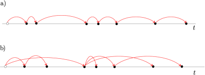
More generally, every spot can deliver $n$ new spots, where $n$ is a random value with Poisson distribution and the mean $\nu$. We describe this situation in terms of (i) standard Hawkes’ process, and (ii) the pulse avalanche model. The temporal distribution of new spots is now governed either by the function $\mu(t)$ of the Hawkes’ process (Hawkes 1971), or $\mu(t,\tau\,|\,t_{0},\tau_{0})$ in the case of avalanches (Poutanen & Fabian 1999). Spots of different generations can appear at the same time.

The difference between the Chinese process and the latter two processes is schematically sketched in Fig. 2. Mathematically, all three examples belong to the class of cluster processes.

3.1 The cluster processes

Point processes are characterised by the generating functional, $\mathcal{G}[.]$, which is defined by its action (Daley & Vere-Jones 2003)

$$\mathcal{G}\big{[}h(x)\big{]}={\rm E}\Big{[}\!\prod\limits_{x_{i}\in{\rm supp}\{N\}}\!\!\!h(x_{i})\Big{]},$$ (21)

where $h(x):\mathcal{X}\rightarrow\mathbb{C}$ is a function satisfying the condition $\left|h(x)\right|\leq 1$.

The functional $\mathcal{G}[.]$ satisfies various relations which can be derived in close analogy with the theory of generating functions of random variables. For our purposes it will be useful to expand $\mathcal{G}[.]$ into a series in terms of factorial measures,

$$\mathcal{G}\left[1+\eta\right]=1+\sum\limits^{\infty}_{k=1}\!\!\int\limits_{\leavevmode\nobreak\ \mathcal{X}^{k}}\!\eta(x_{1})\dots\eta(x_{k})\,M_{[k]}({\rm d}x_{1}\dots\rm dx_{k}).$$ (22)

The cluster processes consist of two point processes. The first one is connected with the counting measure $N_{\rm c}(A)$ and defines the central points $y$ of the clusters. The second process spreads new points around the central point according to the random measure $N(B\,|\,y)$. The complete counting measure is then $N(A)=\int_{\mathcal{X}}N(A\,|\,y)\,N_{\rm c}({\rm d}y)$.

Let $\mathcal{G}\left[h(x)\,|\,y\right]$ be the generating functional of a cluster with the center at $y$,

$$\mathcal{G}\big{[}h(x)\big{]}={\rm E}\Big{[}\int\limits_{\mathcal{X}}\mathcal{G}\big{[}h(x)\,|\,y\big{]}\,N_{\rm c}({\rm d}y)\Big{]}.$$ (23)

If the cluster center process is Poissonian, the latter formula simplifies to

$$\mathcal{G}\big{[}h(x)\big{]}=\exp\Big{\{}-\int\limits_{\mathcal{X}}\big{(}1-\mathcal{G}\left[h(x)\,|\,y\right]\big{)}\,\Lambda_{\rm c}({\rm d}y)\Big{\}},$$ (24)

where $\Lambda_{\rm c}({\rm d}y)$ is the intensity measure of the center process. One can expand the functional (24) in terms of the factorial measure of the cluster,

$$\mathcal{G}\big{[}1+\eta\,|\,y\big{]}=1+\!\sum\limits^{\infty}_{k=1}\int\limits_{\mathcal{X}^{k}}\eta(x_{1})\dots\eta(x_{k})M_{[k]}({\rm d}x_{1}\dots\rm dx_{k}\,|\,y).$$ (25)

Putting Eqs. (22) and (25) into Eq. (24) and collecting the terms with the same order of $\eta(x)$, we find

$$M_{[1]}(A)\! = \!\!\int\limits_{\mathcal{X}}\!M_{[1]}(A\,|\,y)\,\Lambda_{\rm c}\,({\rm d}y),$$ (26)

$$M_{[2]}(A\times B)\! = \!\!\int\limits_{\mathcal{X}}\!M_{[2]}(A\times B\,|\,y)\,\Lambda_{\rm c}\,({\rm d}y)+M_{[1]}(A)\,M_{[1]}(B).$$ (27)

For a stationary process, the intensity measure stays constant, $\Lambda_{\rm c}({\rm d}x)=\lambda_{\rm c}{\rm d}x$, and gives the density of the centers. All factorial moments are shift-invariant in the sense

$$m_{[k]}(x_{1},\dots,\,x_{k}\,|\,y)=m_{[k]}(x_{1}-y,\dots,\,x_{k}-y\,|\,0),$$ (28)

where $m_{[k]}(.\,|\,y)$ is density of $M_{[k]}(.\,|\,y)$. As a result of the shift invariance, density of the first-order moment $m_{1}$ must be also constant. Moreover, we can always choose $y$ in Eq. (28) equal to one of $x_{i}$, so the function $m_{[k]}$ depends on only $k-1$ variables. We define the reduced factorial moments,

$$\breve{m}_{[k]}(u_{1},\dots,\,u_{k-1})=m_{[k]}(0,\,u_{1},\dots,\,u_{k-1}),$$ (29)

and from Eq. (27) it follows that

$$\breve{m}_{[2]}(u)=\lambda\int\limits_{\mathcal{X}}m_{[2]}(y,y+u\,|\,0)\,{\rm d}y+m^{2}_{1}.$$ (30)

Stationarity of the process implies that the second-order measure density depends only on the difference of its arguments,

$$m_{[2]}(t,t^{\prime})=\breve{m}_{[2]}(t-t^{\prime})=c\,(t-t^{\prime})+m_{1}^{2},$$ (31)

where $c(t)$ is an even function.

The second-order measure of a marked cluster process is

$$\!\!\!M_{2}({\rm d}t\,{\rm d}\phi\,{\rm d}r\,{\rm d}\mbox{\boldmath$\xi$}\,{\rm d}t^{\prime}\,{\rm d}\phi^{\prime}\,{\rm d}\mbox{\boldmath$\xi$}^{\prime})=\big{[}\big{(}m_{1}^{2}+c(t-t^{\prime})\big{)}\,G({\rm d}\phi\,{\rm d}r\,{\rm d}\mbox{\boldmath$\xi$})$$

$$\times\,G({\rm d}\phi^{\prime}\,{\rm d}r^{\prime}\,{\rm d}\mbox{\boldmath$\xi$}^{\prime})+m_{1}\,G({\rm d}\phi\,{\rm d}r\,{\rm d}\mbox{\boldmath$\xi$})$$

$$\times\,\delta(t-t^{\prime})\,\delta(\phi-\phi^{\prime})\,\delta(r-r^{\prime})\,\delta(\mbox{\boldmath$\xi$}-\mbox{\boldmath$\xi$}^{\prime})\big{]}\,{\rm d}t\,{\rm d}t^{\prime},$$ (32)

almost identical with that of the Poissonian process. There is only one additional term associated with the function $c(t)$. The resulting spectrum is given by a somewhat lengthy, but still explicit formula. We find stationary cluster processes to be particularly promising as a general scheme, encompassing a broad range of models as special cases. The PSD is

$$\!\!S(\omega)=S_{1}(\omega)+4\pi^{2}m_{1}$$

$$\times\sum\limits_{k,l=-\infty}^{\infty}\int\limits_{\mathcal{K}}e^{i(l-k)\phi}c_{k}(r)\,c^{*}_{l}(r)\,\mathcal{F}_{k}(\omega)\,\mathcal{F}_{l}^{*}(\omega)\,G({\rm d}\phi\,{\rm d}r\,{\rm d}\mbox{\boldmath$\xi$})$$ (33)

with $S_{1}(\omega)\equiv 4\pi^{2}S_{\rm\!P}(\omega)\,Q_{{{}_{\mathcal{K}}}}(\omega)\,{Q_{{{}_{\mathcal{K}}}^{\prime}}}^{\!\!\!*}(\omega)$ and

$$Q_{{{}_{\mathcal{K}}}}(\omega)\equiv\!\sum\limits_{k=-\infty}^{\infty}\!\int\limits_{\mathcal{K}}\!e^{-ik\phi}c_{k}(r)\,\mathcal{F}_{k}(\omega)\,G({\rm d}\phi\,{\rm d}r\,{\rm d}\mbox{\boldmath$\xi$}).$$ (34)

The reduced quadratic factorial moment appears in the formulae for power spectra of cluster processes expressed in terms of $S_{\rm\!P}(\omega)\equiv\mathcal{F}\left[c(t)\right](\omega)=\mathcal{F}\left[\breve{m}_{[2]}(t)-m^{2}_{1}\right](\omega)$. This is directly related to the two-dimensional Fourier transform of the quadratic factorial measure as

$$S_{\rm\!P}(\omega)=\lambda\,\tilde{m}_{[2]}(\omega,-\omega\,|\,0),$$ (35)

where

$$\tilde{m}_{[2]}(\omega,\omega^{\prime}\,|\,0)=\int\limits_{\mathbb{R}^{2}}e^{i(x_{1}\omega+x_{2}\omega^{\prime})}m_{[2]}(x_{1},\ x_{2}\,|\,0)\,{\rm d}x_{1}\,{\rm d}x_{2}.$$ (36)

We will discuss the form of $S_{\rm\!P}(\omega)$, the expression for $m_{1}$, and the resulting PSD in different situations. But before that, we still need to show how the model properties can be detailed in term of marks.

3.2 Marks as a way to specify the model properties

Until now the variability patterns have been restricted only by very general properties of the assumed process. This means that the model is kept in a very general form. However, formulae (14) and (33) are too general for any practical use. Their main value is after defining special cases. Then these formulae can be readily applied to derive the analytical form of the PSD. Such special cases are conveniently defined by means of marks. We discuss possible choices of the mark distribution, $G({\rm d}r\,{\rm d}\phi\,{\rm d}\mbox{\boldmath$\xi$})$.

We can simplify the situation by assuming axial symmetry. Therefore, all statistical properties should depend only on the radius (the azimuthal part of $G$ is constant). The distribution of marks has now the form

$$G({\rm d}r\,{\rm d}\phi\,{\rm d}\mbox{\boldmath$\xi$})=\frac{1}{2\pi}\,\zeta_{\rm R}(\mbox{\boldmath$\xi$}\,|\,r)\,\rho(r)\,{\rm d}r\,{\rm d}\phi\,{\rm d}\mbox{\boldmath$\xi$},$$ (37)

where $\zeta_{\rm R}(\mbox{\boldmath$\xi$}\,|\,r)$ is the reduced probability density of the remaining parameters. To illustrate this case more clearly, we will now examine the phenomenological model of Abramowicz et al. (1991) and Zhang & Bao (1991), which can be considered as representation of the spotted accretion disc.

3.3 Example 2: a spotted disc

Let $n(r)$ be an average number of spots at radius $r$, each of them shining with the average intensity $I_{\rm M}(r)$ for average duration $\tau_{\rm M}(r)$. Let us further assume that these characteristics scale with the radius as power laws:

$$n(r)=A_{n}\,r^{\alpha_{n}},\quad\tau_{\rm M}(r)=A_{\tau}\,r^{\alpha_{\tau}},\quad I_{\rm M}(r)=A_{I}\,r^{\alpha_{I}}$$ (38)

(here, $\alpha$s and $A$s are constants). This setup falls within the category of models described by Eq. (2), with the profile function $I(t,r,\tau)$ and the mark distribution $G({\rm d}r\,{\rm d}\phi\,{\rm d}\tau)$. The first two relations (38) prescribe the conditional marginals of $G$, i.e.,

$$n(r)=\lambda\,\rho(r),\quad\tau_{\rm M}(r)=\int\limits_{\tau_{\rm min}(r)}^{\tau_{\rm max}(r)}\tau\,\zeta_{\rm R}(\tau\,|\,r)\,{\rm d}\tau,$$ (39)

where the integration limits can depend explicitly on $r$. The third equation determines the amplitude of the profile function,

$$I(t,r,\tau)=A_{I}\,r^{\alpha_{I}}\,g(t,\tau)\,\theta(t).$$ (40)

The dependency on $\tau$ is not determined uniquely. In order to obtain an explicit form of $G$ we have to go beyond the model of Abramowicz et al. (1991) by assuming the distribution of $\tau$,

$$\zeta_{\rm R}(\tau\,|\,r)=K(r)\,\tau^{-p}.$$ (41)

The normalisation constant then equals

$$K(r)=\frac{1-p}{\tau_{\rm max}^{1-p}(r)-\tau_{\rm min}^{1-p}(r)},$$ (42)

and for $\tau_{\rm M}(r)$ we find

$$\tau_{\rm M}(r)=K(r)\,\int\limits_{\tau_{\rm min}(r)}^{\tau_{\rm max}(r)}\tau^{1-p}{\rm d}\tau=\frac{1-p}{2-p}\frac{\tau_{\rm max}^{2-p}(r)-\tau_{\rm min}^{2-p}(r)}{\tau_{\rm max}^{1-p}(r)-\tau_{\rm min}^{1-p}(r)}.$$ (43)

The mean, $\tau_{\rm M}(r)$, must satisfy Eqs. (38) and (43). The choice of

$$\tau_{\rm min}(r)=C_{\rm min}r^{\alpha_{\tau}},\quad\tau_{\rm max}(r)=C_{\rm max}r^{\alpha_{\tau}}$$ (44)

is consistent with both equations. Constants $C_{\rm min}$, $C_{\rm max}$ and $A_{\tau}$ are bound by the relation

$$A_{\tau}(2-p)(C_{\rm max}^{1-p}-C_{\rm min}^{1-p})=(1-p)(C_{\rm max}^{2-p}-C_{\rm min}^{2-p})$$ (45)

Because $C_{\rm min}$ and $C_{\rm max}$ are positive, we can write

$$C_{\rm min}=C,\quad C_{\rm max}=\gamma C,$$ (46)

$$C = A_{\tau}\frac{2-p}{1-p}\frac{\gamma^{1-p}-1}{\gamma^{2-p}-1},$$ (47)

$$K(r) = \frac{1-p}{\gamma^{1-p}-1}\left(Cr^{\alpha_{\tau}}\right)^{p-1}.$$ (48)

Therefore, by substituting back to Eq. (41), we obtain

$$\zeta_{\rm R}(\tau\,|\,r)\,\rho(r) = \frac{\alpha_{n}+1}{\left(r_{\rm max}^{\alpha_{n}+1}-r_{\rm min}^{\alpha_{n}+1}\right)}\frac{1-p}{\gamma^{1-p}-1}$$ (49)

$$\times \left(\frac{2-p}{1-p}\frac{\gamma^{1-p}-1}{\gamma^{2-p}-1}A_{\tau}\right)^{p-1}\,\tau^{-p}\,r^{(p-1)\alpha_{\tau}+\alpha_{n}},$$

where the definition domain is a set

$$\Xi=\left\{(r,\xi(r))\,|\,r\in\langle r_{\rm min},r_{\rm max}\rangle,\xi(r)\in Cr^{\alpha_{\tau}}\langle 0,\gamma\rangle\right\}.$$ (50)

We can set $p=1$ as a specific example. This value of the power-law index is special in the sense that neither short nor long timescales dominate the PSD, as we see from Eq. (42):

$$C=A_{\tau}\frac{\ln\gamma}{\gamma-1},\quad K(r)=\frac{1}{\ln\gamma}.$$ (51)

By substituting back to Eq. (41) we obtain

$$\zeta_{\rm R}(\tau\,|\,r)\,\rho(r)=\frac{\alpha_{n}+1}{\ln\gamma\left(r_{\rm max}^{\alpha_{n}+1}-r_{\rm min}^{\alpha_{n}+1}\right)}\,r^{\alpha_{n}}\,\tau^{-1}.$$ (52)

Knowing the concrete form of the distribution of marks, we perform the integration over $\xi$. As $I(t,r)$ does not explicitly depend on azimuthal angle, the integration is simplified. Denoting

$$d_{n}(r)=\frac{1}{2\pi}\int\limits_{0}^{2\pi}e^{in[\phi+\Omega(r)\delta t(r,\,\phi)]}\,{\rm d}\phi,$$ (53)

we rewrite the PSD formula (14) in the final form

$$S(\omega) = 4\pi^{2}n\!\!\!\sum\limits_{k,l=-\infty}^{\infty}\,\int\limits_{r_{\rm min}}^{r_{\rm max}}\!c_{k}(r)\,c^{*}_{l}(r)\,d_{k-l}(r)$$ (54)

$$\times\int\limits_{\Xi}\!\mathcal{F}_{k}(\omega)\,\mathcal{F}_{l}^{*}(\omega)\,\zeta_{\rm R}(\mbox{\boldmath$\xi$}\,|\,r)\,{\rm d}\mbox{\boldmath$\xi$}\,\rho(r)\,{\rm d}r.$$

We find the coefficients by direct evaluation,

$$d_{n}(r)=\frac{1}{2\pi}\int\limits_{0}^{2\pi}e^{iny}\left[1+\Omega(r)\,\frac{\partial\delta t(\phi(y),r)}{\partial{\phi}}\right]^{-1}{\rm d}\phi$$ (55)

with $y=\phi+\Omega(r)\,\delta t(\phi,r)$. We note that the term (55) corresponds to the effect of delay amplification in terminology of Dovčiak et al. (2008). It influences the observed signal from a source moving (i.e., orbiting) near a black hole.

4 Results for the model PSD

4.1 Model driven by the Chinese process

Let us denote $\psi$ the probability that an existing spot generates a new one, and $q_{k}$ the probability that a family of spots consists of exactly $k$ members. The value $q_{k}$ obeys the geometrical distribution, $q_{k}=\psi^{k}(1-\psi)$.

We interpret probability density $p(t)$ of the delay between successive spots as a mean number of first-generation spots that occur at the ignition time $t>0$, where $t=0$ is a moment of ignition of the parent spot. Analogically, $p(t)\star p(t)$ is the mean number of second-generation spots. For a sequence of $k$ spots, we obtain the intensity measure

$$m_{1}(t\,|\,0,k)=\sum\limits_{j=0}^{k}p^{\star j}(t),$$ (56)

where $p^{\star k}(t)$ is the $k$th convolutionary power of $p(t)$. We can write $m_{1}$ in the form

$$m_{1}(t\,|\,0)=\sum\limits_{k=0}^{\infty}q_{k}\,m_{1}(t\,|\,0,k).$$ (57)

Convolution of two functions can be calculated via the Fourier image. Defining $\tilde{p}(\omega)=\mathcal{F}\left[p(t)\right](\omega)$ we get

$$\tilde{m}_{1}(\omega\,|\,0)=(1-\psi)\sum\limits_{k=0}^{\infty}\psi^{k}\sum\limits_{j=0}^{k}\tilde{p}^{j}(\omega)=\frac{1}{1-\psi\tilde{p}(\omega)}.$$ (58)

From this we find

$$\int\limits_{0}^{\infty}m_{1}(t\,|\,0)\,{\rm d}t = \tilde{m}_{1}(\omega\,|\,0)_{|\omega=0}=\frac{1}{1-\psi},$$ (59)

$$\int\limits_{0}^{\infty}t\,m_{1}(t\,|\,0)\,{\rm d}t = -i\,\frac{\rm d}{{\rm d}\omega}\tilde{m}_{1}(\omega\,|\,0)_{|\omega=0}=\frac{\psi}{\left(1-\psi\right)^{2}}\,{\rm E}[t].$$ (60)

The meaning of integral (59) is the average number of spot offsprings in the whole avalanche. The meaning of the last integral is the average duration of the avalanche.

Calculation of the quadratic measure is a less intuitive procedure. We start from the generating functional (21) of the process,

$$\mathcal{G}\left[h(t)\,|\,0\right]=\sum\limits_{l=0}^{\infty}q_{l}\,h(0)\,\mathcal{G}_{l}[h(t)],$$ (61)

where $\mathcal{G}_{l}[.]$ denotes a generating functional of finite renewal process with $l$ points (see chapt. 5 in Daley & Vere-Jones 2003).

Substituting $h(t)=1-\eta(t)$ in the expansion (22), we obtain the Fourier image

$$\tilde{m}_{[2]}(\omega,\omega^{\prime}\,|\,0)\!=\!\frac{\psi\big{[}\tilde{p}(\omega)+\tilde{p}(\omega^{\prime})-2\psi\tilde{p}(\omega)\tilde{p}(\omega^{\prime})\big{]}}{\big{[}1-\psi\tilde{p}(\omega)\big{]}\big{[}1-\psi\tilde{p}(\omega^{\prime})\big{]}\big{[}1-\psi\tilde{p}(\omega+\omega^{\prime})\big{]}}.$$ (62)

This equation allows us to find the second-order measure. The PSD is then given by Eqs. (33)–(34) with

$$m_{1} = \frac{\lambda}{1-\psi},$$ (63)

$$S_{\rm\!P}(\omega) = \frac{2\lambda\psi\,\big{[}\Re e\,\big{\{}\tilde{p}(\omega)\big{\}}+\psi\,|\,\tilde{p}(\omega)\,|\,^{2}\big{]}}{(1-\psi)\big{[}1-2\psi\,\Re e\,\big{\{}\tilde{p}(\omega)\big{\}}+\psi^{2}\,|\,\tilde{p}(\omega)\,|\,^{2}\big{]}}.$$ (64)

Equation (64) can be cast in the form

$$S_{\rm\!P}(\omega)=\lambda\,\frac{|\tilde{m}_{[1]}(\omega\,|\,0)|^{2}\,\big{(}1-\psi^{2}\,|\tilde{p}(\omega)|^{2}\big{)}-1}{1-\psi}.$$ (65)

Figure 3: Power spectra from the spot model in which the birth and duration of spots are governed by the market Hawkes process with the exponential infectivity (76). Values of $\alpha$ are given on top of the plots. Frequency is given in geometrical units (see the text for its scaling to physical units). In each frame, the four curves correspond to different values of $\nu$; from bottom to top $\nu=0.1$, $0.5$, $0.9$, and $0.99$. The mean number of spontaneous spots has been set to $\lambda=(2\pi)^{-1}$. The relative normalisation of these curves scales as the mean number of all spots, i.e. proportionally to $1/(1-\nu)$. Left: the case when all profiles $I(t)$ are identical; $\tau=1$, i.e. $\zeta(\tau)=\delta(\tau-1)$. Right: the case when the life-times of spots are distributed uniformly, i.e. according to $\zeta(\tau)=1/(\tau_{\rm max}-\tau_{\rm min})$, between $\tau_{\rm min}=0.01$ and $\tau_{\rm max}=1$.

Figure 4: Graphs of the model PSD as in the previous figure, but for the case of Hawkes process with the power law infectivity (80). Parameter values $\beta$ are given on top of each panel; values of $\nu$ are as in Fig 3. All spots have the same (exponential) profile, as in the previous figure. For $\beta\gtrsim 1.5$ we notice the new profile resembles a power law that develops in between the two peaks. However, this situation is rather rare within the parameter space of our models. By parameter tuning – e.g., by setting $\nu\rightarrow 1$, which means enhancing the contribution of avalanches while suppressing the importance of spontaneous parent spots – the extent of the flat part of the PSD profile (like the one seen for $\beta=1.5$) can be stretched farther towards small frequencies.

4.2 Model driven by the Hawkes process

Hawkes’ process (Hawkes 1971; Brémaud & Massoulié 2002) is more complicated than the previous example because it consists of two types of events. First, new spots are generated by the Poisson process operating with intensity $\lambda$ (let us denote $t_{0}$ the moment of ignition). Second, an existing spot can give birth to new one at a later time, $t$, according to the Poisson process with varying intensity $\mu(t-t_{0})$.

The mean number of events is

$$m(t)=\lambda+\sum\limits_{i,t_{i}<t}\mu(t-t_{i})=\lambda+\int\limits_{-\infty}^{\infty}\mu(t-x)\,N({\rm d}x).$$ (66)

In analogy with Eq. (60) we define the characteristic time of avalanche $t_{\rm a}$. It can be proven that $t_{\rm a}$ is related to the characteristic time of the infectivity $t_{\rm i}$:

$$t_{\rm a}=\frac{\int\limits_{0}^{\infty}t\,m_{1}(t\,|\,0)\,{\rm d}t}{\int\limits_{0}^{\infty}m_{1}(t\,|\,0)\,{\rm d}t}=\frac{\nu}{1-\nu}\frac{\int\limits_{0}^{\infty}t\,\mu(t)\,{\rm d}t}{\int\limits_{0}^{\infty}\mu(t)\,{\rm d}t}=\frac{\nu}{1-\nu}\,t_{\rm i}.$$ (67)

For a stationary process, the first-order moment density is constant. Averaging the relation (66) we find

$$m_{1}=\frac{\lambda}{1-\nu},\quad\nu=\int\limits_{0}^{\infty}\mu(t)\,{\rm d}t.$$ (68)

The meaning of $\nu$ is the mean number of the offsprings. Clearly, it satisfies the normalisation $\int\mu(x)\,{\rm d}x\equiv\nu\leq 1$.

The generating functional of the cluster of the Hawkes process fulfils the integral equation,

$$\mathcal{G}\big{[}h(x)\,|\,0\big{]}=h(0)\exp\Big{\{}\!-\!\int\limits_{-\infty}^{\infty}\left(1-\mathcal{G}\left[h(x)\,|\,y\right]\right)\,\mu(y)\,{\rm d}y\Big{\}}.$$ (69)

Substituting $h(x)=1+\eta(x)$ and expanding both sides into the series (25) we find

$$m_{[1]}(t\,|\,0) = \int\limits_{-\infty}^{\infty}m_{[1]}(t\,|\,y)\,\mu(y)\,{\rm d}y+\delta(t),$$ (70)

$$m_{[2]}(t,t^{\prime}\,|\,0) = \int\limits_{-\infty}^{\infty}m_{[2]}(t,t^{\prime}\,|\,y)\,\mu(y)\,{\rm d}y$$ (71)

$$+m_{[1]}(t\,|\,0)\,m_{[1]}(t^{\prime}\,|\,0)-\delta(t)\,\delta(t^{\prime}).$$

Figure 5: Decomposition of the total PSD curve, $S_{\!\rm t}(\omega)$, into a product of two terms which are responsible for the two peaks in the final profile (see Eq. (83)). Left: this case corresponds to $\alpha=10$, $\nu=0.5$ curve shown in the bottom–left panel of Fig. 3. Right: this case corresponds to $\beta=1.9$ and $\nu=0.99$ curve in the middle–right panel of Fig. 4. Similar behaviour of the PSD profile is typical in our model, although in some cases only one peak dominates the spectrum whereas the other one is suppressed.

To complete the calculation we solve the integral equation (70) for $m_{[1]}(x\,|\,0)$. Because this is a linear convolutional integral equation, it can be solved efficiently by using the Fourier transform:

$$\tilde{\mu}(\omega) = \int\limits_{-\infty}^{\infty}e^{-i\omega t}\mu(t)\,{\rm d}t,$$ (72)

$$\tilde{m}_{[1]}(\omega\,|\,0) = \int\limits_{-\infty}^{\infty}e^{-i\omega t}m_{[1]}(t\,|\,0)\,{\rm d}t=\frac{1}{1-\tilde{\mu}(\omega)}.$$ (73)

For the Fourier transform of the quadratic factorial measure we find

$$\tilde{m}_{[2]}(\omega,\omega^{\prime}\,|\,0)=\frac{\tilde{m}_{[1]}(\omega\,|\,0)\tilde{m}_{[1]}(\omega^{\prime}\,|\,0)-1}{1-\mu(\omega+\omega^{\prime})}.$$ (74)

Again, the PSD is given by Eqs. (33), (34), and (68) with

$$S_{\rm\!P}(\omega)=\lambda\,\frac{|\tilde{m}_{[1]}(\omega\,|\,0)|^{2}-1}{1-\nu}.$$ (75)

Comparing this equation describing the Hawkes process PSD with the corresponding Eq. (65) for the case of the Chinese process, we reveal a subtle difference between the two mechanisms. It turns out that the high-frequency limit is identical for both of them, however, the difference grows as one proceeds towards the low-frequency end of the PSD domain.

Figure 6: The pulse avalanche model for the uniform probability density $\zeta(\tau)$, constrained by limits $\tau_{\rm min}=0.01$ and $\tau_{\rm max}=1$. Left: the PSD calculated from the formulae (33) and (86). Right: the ratio between the PSD of the pulse avalanche process to the Hawkes process; in the latter the exponential infectivity $\mu(t)$ is related to the corresponding infectivity of the pulse avalanche process by $\mu(t)=\mu(t\,|\,\bar{\tau})$.

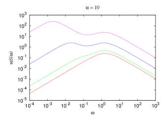
For the exponential form of infectivity measure,

$$\mu(t)=\nu\sigma\,e^{-\sigma t}\,\theta(t),$$ (76)

we obtain the explicit expression of

$$\tilde{m}_{[1]}(\omega\,|\,0) = 1+\frac{\nu\sigma}{\sigma(1-\nu)+i\omega},$$ (77)

$$S_{\rm\!P}(\omega) = \frac{\nu\,(2-\nu)\,\sigma^{2}}{(1-\nu)^{2}\,\sigma^{2}+\omega^{2}}\,\frac{\lambda}{1-\nu},$$ (78)

where $\sigma>0$ is a constant.

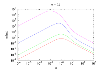
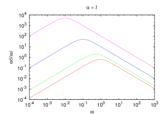
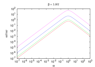
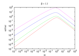
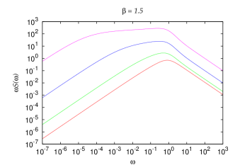
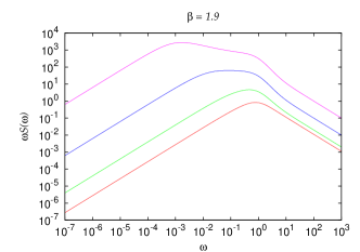
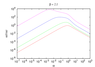
Figure 3 shows the resulting PSD of this model in a logarithmic plot of $\omega S(\omega)$ versus $\omega$. Here we can study the occurrence of break frequency where the PSD slope changes depending on the model parameters. Light curve profiles of individual spots were chosen as exponentials, $I(t)=I_{0}\exp(-t/\tau)\,\theta(t)$, where $\tau$ is random value with probability density $\zeta(\tau)$ and the mean $\bar{\tau}$. The characteristic time of infectivity, $t_{i}=\sigma^{-1}$, is set to be $t_{i}=\alpha\,\bar{\tau}$. In general, we can identify two characteristic frequencies in the PSD. The first one corresponds to the characteristic frequency of the profile $I(t)$ (in our case this frequency is given by $1/\bar{\tau}$), the second one is given by the characteristic frequency of the avalanches ($1/t_{\rm a}$).

We remind the reader that this plot (as well as the subsequent figures 4–6) does not include general relativity effects; they will be recovered later in the paper. This is merely to simplify calculations – the relativistic effects complicate the derivation of the analytical formula for the PSD and it is somewhat difficult to distinguish them from the intrinsic properties of the signal.

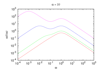
The typical form of the model PSD resembles a Lorentzian or doubly-Lorentzian profile at central frequencies. In most cases, there is only one break in the spectra corresponding to the characteristic frequency of the profiles $I(t)$. When two peaks are visible, as we notice from Fig. 3 and Eq. (78), two characteristic frequencies occur. The upper frequency is scaled to unity in our figures; this peak corresponds to the e-folding time of the exponentially decaying spots, i.e. $I(t)\propto\exp(-t/\tau)$. The lower frequency peak is then set by a combination of two timescales,

$$\frac{\bar{\tau}}{t_{\rm a}}=\frac{1-\nu}{\alpha},$$ (79)

where $\bar{\tau}\equiv{\rm E}[\tau]$. Notice that the model is sufficiently complex, and so one cannot easily disentangle the two timescales in any straightforward way directly from the PSD.

Another natural choice of infectivity is a power-law function of the form

$$\mu(t)=\frac{K}{(t+L)^{\beta}}\,\theta(t),$$ (80)

where $\beta$, $K$, and $L$ are positive constants satisfying

$$\beta>1,\quad K=\nu\,(\beta-1)\,L^{\beta-1}.$$ (81)

One can thus ask how the PSD form depends on the assumptions about the form of the infectivity function $\mu$. For every $b>0$ the function (80) satisfies $\left.\mu(t)\right|_{L=b}=b^{-1}\left.\mu(t/b)\right|_{L=1}$. Therefore, we can set $L=1$ without any loss of generality (the value of $L$ can be recovered by a simple rescaling of the result).

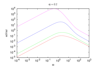
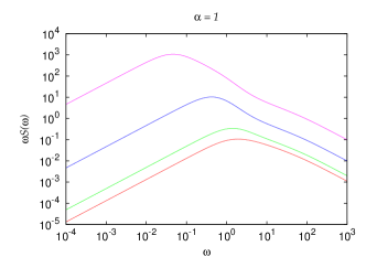
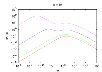
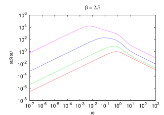
We note that the characteristic times $t_{\rm a}$ and $t_{\rm i}$, as defined in Eq. (67), diverge for the infectivity (80) and $1<\beta\leq 2$. In this case, $t_{\rm a}$ does not exist. Again, we derive an analytical form of the PSD for the adopted infectivity function. The procedure is entirely analogical as above, but we do not give the explicit form of $S_{\rm\!P}(\omega)$ because the final formula is rather complicated. The resulting PSD curves with the power-law infectivity are plotted in Fig. 4.

It is also interesting to note at this point, how the peaks of the PSD move when the model parameters are shifted. For example, see the panel $\alpha=1$ of Fig. 3. Although in this case the two timescales are equal to each other, changing the other parameter, $\nu$, from $0.1$ to $0.99$ brings the peak over two orders of magnitude. In other words, the maximum of the PSD can appear at a frequency lower than the inverse of the spot decay time. The frequency shift of the peaks is again given by factor $t_{\rm a}/\bar{\tau}$, as explained in Eq. (79).

In order to understand better the behaviour of the PSD peaks, we rewrite Eq. (33) in the form

$$S(\omega)=m_{1}\,{\rm E}\big{[}\big{|}\mathcal{F}[I](\omega)\big{|}^{2}\big{]}+S_{\rm P}(\omega)\;\big{|}{\rm E}\big{[}\mathcal{F}[I](\omega)\big{]}\big{|}^{2}$$ (82)

(i.e., relativistic effects neglected). Equation (82) can be simplified by assuming that all spots have the identical, exponentially decaying light curves, $I(t,\tau)=I_{0}\,e^{-t/\tau}\,\theta(t)$. We obtain

$$S(\omega)=S_{\rm L}(\omega)\,\big{(}m_{1}+S_{\rm P}(\omega)\big{)},$$ (83)

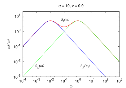
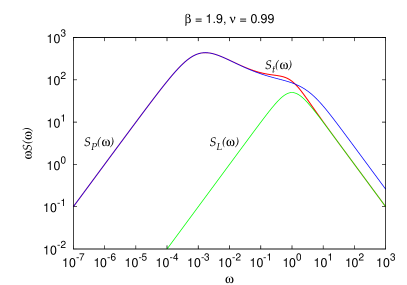
where $S_{\rm L}(\omega)=\tau^{2}/(1+\omega^{2}\tau^{2})$ is the Lorentzian PSD, and $m_{1}$ is a constant (see the discussion following Eq. (28)). In this simple case the two terms, $S_{\rm L}(\omega)$ and $S_{\rm P}(\omega)$, give rise to two comparably significant peaks, although their amplitudes are generally different. The situation is shown in Fig. 5. The left panel is particularly transparent because it shows the Hawkes process with exponential infectivity, for which $S_{\rm P}(\omega)$ adopts the Lorentzian shape, dominating the spectrum at frequencies where $S_{\rm L}(\omega)\approx 1$. Therefore, Eq. (83) is effectively a sum of two identical Lorentzians. However, this example does not apply to a general case when the amplitudes of the PSD peaks can be very different. In the right panel, we note that $S_{\rm{}P}(\omega)$ itself dominates the whole spectrum and has a complicated (non-Lorentzian) shape.

Figure 7: Upper panels: Power spectra from the Poisson-driven spot model, calculated for a thin accretion disc extending between radii $r=6M$ and $r=100M$ (in geometrical units), for three inclinations $\theta_{\rm o}$. The purpose of this plot is to demonstrate a general agreement between the PSD calculated from the model light curve and from the analytical formula. The wiggly (red) curve is a result of direct numerical simulation, including the relativistic effects. The smooth (blue) curve is the analytical result, derived from Eq. (14) by specifying the probability density function $\zeta(\tau)\propto 1/\tau$. The vertical (magenta) lines represent the Keplerian orbital frequencies, $\Omega(r)$, at the inner and the outer edges of the disc. Lower panels: Power spectra from the Hawkes process with the exponential infectivity ($\alpha=7$, $\nu=0.8$). The analytical curve was calculated by using formula (33) and assuming the same probability density function $\zeta(\tau)\propto 1/\tau$. In all panels we set $\tau_{\rm min}=300$, $\tau_{\rm max}=5000$.

Figure 8: The analytical curves of the PSD profiles are plotted, with relativistic effects included. In order to allow comparison with previous figures, we selected appropriate combinations of the model parameters: the infectivity $\alpha$, the mean number of secondary spots $\nu$, and the spot distribution are the same as in Fig. 3. The inclination $\theta_{\rm o}$ and the spot distribution as in Fig. 7. The vertical lines again indicate the range of orbital frequencies corresponding to the assumed range of radii, $6M<r<100M$, where the spots are distributed. The analytical form is quick to evaluate, hence it is convenient to obtain the PSD form for variety of different situations.

Figure 9: The ratio $R_{\rm{}S}(\omega)$ of PSD computed with and without relativistic effects. The difference is most visible around intermediate frequencies; Keplerian orbital frequencies at the outer/inner edges of the spot radial distribution are again indicated by vertical lines. The arrangement of panels and the assumed parameter values are the same as in the previous Fig. 8. In particular, the vertical lines indicate the minimum and the maximum orbital frequencies corresponding to the outer and the inner edges of the spot distribution.

4.3 The pulse avalanche model

The pulse avalanche model was discussed in the context of various astronomical objects whose light curves exhibit signs of stochastic behaviour. They are, namely, gamma-ray bursting sources (Stern & Svensson 1996). As a framework to describe the timing characteristics of accreting black holes, the model was studied by Poutanen & Fabian (1999). Details of the process are different in those two papers and our description is closer to the latter one.

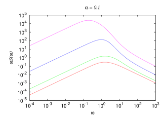
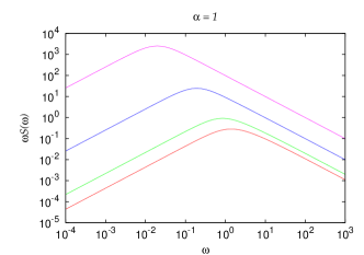
The basic properties of the pulse avalanche model can be summarised as follows. (i) The observed signal consists of pulses of the form $I(t,\tau)=I_{0}\,g(t,\tau)\,\theta(t)$, where $\tau$ is their characteristic duration. (ii) Each pulse gives birth to $b$ baby pulses; the number of baby pulses varies, obeying the Poisson distribution $P(b)=\nu^{b}/(b!\,e^{\nu})$ with the mean value $\nu$. (iii) The baby pulses are delayed with respect to the parent ones by $\Delta t$, which is a random value with exponential distribution, $P(\Delta t)=(\alpha\tau_{0})^{-1}e^{-\Delta t/(\alpha\tau_{0})}$. (iv) Some pulses occur spontaneously, according to the Poisson process operating at the mean rate $\lambda$. Finally, (v) temporal constants, $\tau$, for all pulses are mutually independent and drawn from the same distribution function, $\zeta(\tau)$. Such a process is clearly of the form (2).

The underlying point process is a cluster process operating on the set $\mathbb{R}\times\langle\tau_{\rm min},\,\tau_{\rm max}\rangle$ with properties similar to the Hawkes process. (In fact, we will see below that the Hawkes process can be considered as a special case of the pulse avalanche process.) The center process is the Poissonian one, and its intensity is $\lambda_{\rm c}(t,\tau)=\lambda\zeta(\tau)$. The clusters are driven by the Poissonian branching process (Cox & Miller 1965) with the parameter measure

$$\mu(t,\tau\,|\,t_{0},\tau_{0})=\frac{\nu\,\zeta(\tau)}{\alpha\tau_{0}}\,\exp\Big{\{}-\frac{t-t_{0}}{\alpha\tau_{0}}\Big{\}}\;\theta(t-t_{0}).$$ (84)

One can prove, by direct integration, that

$${\rm E}\big{[}\Delta t\,|\,t_{0},\tau_{0}\big{]}\! = \!\frac{1}{\nu}\int\limits_{-\infty}^{\infty}\!\int\limits_{\tau_{\rm min}}^{\tau_{\rm max}}\!(t-t_{0})\,\mu(t,\tau\,|\,t_{0},\tau_{0})\,{\rm d}\tau\,{\rm d}t=\alpha\tau_{0},$$

$${\rm E}\big{[}b\,|\,t_{0},\tau_{0}\big{]}\! = \!\int\limits_{-\infty}^{\infty}\int\limits_{\tau_{\rm min}}^{\tau_{\rm max}}\mu(t,\tau\,|\,t_{0},\tau_{0})\,{\rm d}\tau\,{\rm d}t=\nu.$$ (85)

In analogy to Eqs. (70) and (71) one can derive a set of linear integral equations for the first and second order moments of the cluster process. The chosen form (84) of the kernel $\mu(t,\tau\,|\,t_{0},\tau_{0})$ greatly simplifies the task, as it can be again transformed into a convolutory form and solved in the Fourier domain.

The resulting functions $\tilde{m}_{[1]}$ and $\tilde{m}_{[2]}$ are complicated and their inverse Fourier transforms can be directly found only in very special cases, e.g. by assuming $\zeta(\tau)=\delta(\tau-a)$. In that case the pulse avalanche model is transformed into the Hawkes process with the exponential infectivity measure.

Fortunately, we do not need the explicit form of the moments to find the final formula for the PSD. This result is provided by Eq. (33) with

$$S_{\!1}(\omega)=4\pi^{2}\!\!\int\limits_{\tau_{\rm min}}^{\tau_{\rm max}}\int\limits_{\tau_{\rm min}}^{\tau_{\rm max}}\!\!S_{\rm\!P}(\omega,\tau,\tau^{\prime})\,Q_{{{}_{\mathcal{K}}}}(\omega,\tau)\,Q_{{{}_{\mathcal{K}}}^{\prime}}^{*}(\omega,\tau^{\prime})\;{\rm d}\tau\;{\rm d}\tau^{\prime}$$ (86)

and

$$S_{\rm\!P}(\omega,\tau,\tau^{\prime}) = \frac{\lambda}{1-\nu}\,\zeta(\tau)\,\zeta(\tau^{\prime})\big{[}f_{1}(\omega)\,|f_{2}(\omega)|^{2}$$ (87)

$$+\frac{\nu}{1-i\alpha\tau\omega}\,f_{2}(\omega)+\frac{\nu}{1+i\alpha\tau^{\prime}\omega}\,f_{2}^{*}(\omega)\big{]},$$

$$f_{1}(\omega) = \int_{\tau_{\rm min}}^{\tau_{\rm max}}\frac{\nu^{2}\,\zeta(y)}{1+\alpha^{2}\omega^{2}y^{2}}\,{\rm d}y,$$ (88)

$$f_{2}(\omega) = \Big{[}1-\int_{\tau_{\rm min}}^{\tau_{\rm max}}\frac{\nu\zeta(y)}{1+i\alpha\omega y}\,{\rm d}y\Big{]}^{-1}.$$ (89)

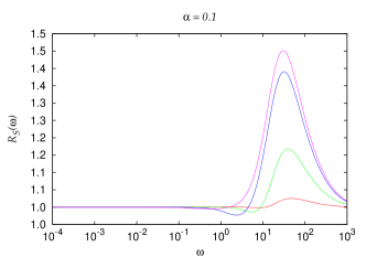
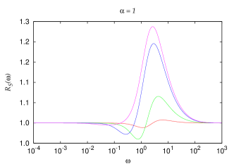
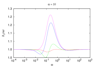
We show several graphs of the resulting model PSD curves in Fig. 6. The overall form of the PSD resembles the previous examples derived for the Hawkes process, although they are not the same. The two models – the pulse avalanche process and the Hawkes process – are identical in their high-frequency and low-frequency limits, but they differ from each other in the middle range of frequency. In order to demonstrate the difference in a clear way we plot the ratio of the models in the right column. Fig. 6 assumes $\zeta(\tau)=1/(\tau_{\rm max}-\tau_{\rm min})$. We also studied the case of $\zeta(\tau)=[\tau\ln(\tau_{\rm max}/\tau_{\rm min})]^{-1}$ and we found that the general form of the PSD profiles exhibits very similar trends. We see only quite minor differences in the limiting slopes of the PSD and in the overall PSD shape in the middle range of frequencies. Therefore, we do not show these plots here (see Pecháček 2008).

4.4 PSD with relativistic effects

Relativistic effects influence the photon energy in the course of light propagation through the curved spacetime, towards a distant observer. In this paper we consider only the energy-integrated light curves, but even those are affected because the energy shifts modify the observed flux level. Furthermore, light rays are bent as they pass near the black hole, causing the light-focusing effect. In consequence the observed light curves differ from their intrinsic profiles produced at the point of emission, and this further complicates the decomposition of the PSD spectrum into elementary components. Therefore, in general the power spectrum cannot be rigorously expressed as a combination of Lorentzians. However, in most circumstances the relativistic effects are not very prominent – only a small fraction of rays passing very close to the black hole horizon and those crossing the caustics are affected. One expects that they cannot be ignored if the accretion disc extends down to the innermost stable orbit or if some non-negligible emission arises below that orbit. Also, high-inclination objects are affected more because in those cases the disc is seen edge-on and the intrinsic fluctuations of the emission are considerably amplified.

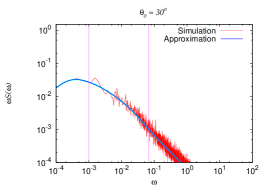
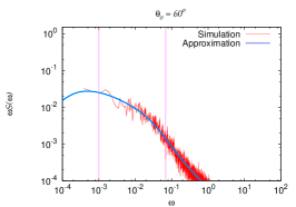
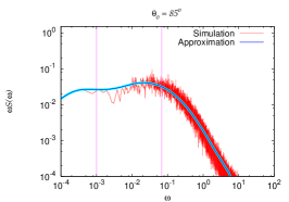
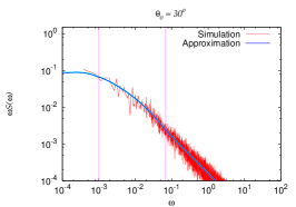
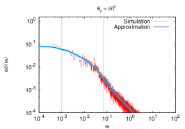
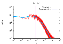
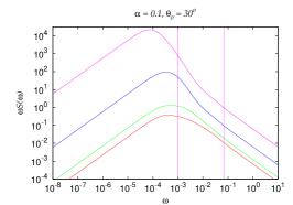
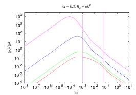
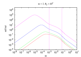
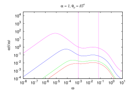
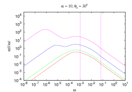
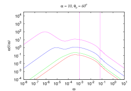
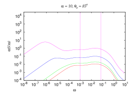
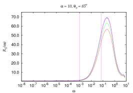
Exemplary power spectra, including the relativistic effects are modelled in Fig. 7 where the numerical simulation is compared with the analytical result. The upper panels assume that orbiting spots are generated by Poissonian process; the lower ones show the PSD derived from Eq. (33). The assumed radial distribution of the spots was $\rho(r)=\rho_{0}\,(1-\sqrt{6/r})\,r^{-2}$, where $\rho_{0}$ is normalisation constant. It turns out that the relativistic effects influence the final PSD especially at high frequencies and high inclinations.

We remind the reader that frequencies in these plots are given in geometrical units (in physical units frequencies scale inversely with the mass of the black hole). We notice that a high-frequency part of the spectrum decays as $\omega S(\omega)\propto\omega^{-1}$, whereas the break occurs towards lower frequencies. These plots provide us with graphical comparisons between the analytical form and the corresponding results of numerical simulations. We note that the adopted approximation of relativistic effects (Pecháček et al. 2005) holds for moderate inclination ($\lesssim 70$ deg). It loses accuracy when the view angle becomes almost edge-on, although the main trend of the PSD remains unchanged.

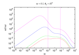
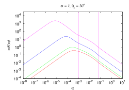
The main advantage of the analytical method is, obviously, in the possibility of obtaining a general form of the PSD, including the relativistic effects. We are ale to search systematically through the vast parameter space of different models for which the model PSD can be explored across a wide range of frequencies. We take the advantage of this approach and plot variety of profiles in Fig. 8. Here, we omit the numerically-simulated curves of the previous figure, so the entire graph is constructed very efficiently. We assumed that spots are generated by the Hawkes mechanism.

Basic trends of the PSD shape are readily recognised. In particular, the curves have either one or two maxima, prominence and position of which changes with parameters. Notice, for example, the bottom right panel in which the PSD is almost flat over several decades of frequency, well below the typical orbital frequency in the disc (vertical lines denote the Keplerian frequencies at the edges of the assumed spot distribution). The flattish part of the spectrum can be extended further, to lower frequencies, by enlarging the $\nu$ parameter towards unity, i.e., by protracting the sequence of avalanches. Next, for large inclinations we notice that relativistic effects produce a prominent bump. This feature occurs near the orbital frequency of the inner disc. Relativistic effects are the main cause of differences between this figure and Fig. 3, in which those effects were neglected.

As already mentioned, general relativity affects mainly the high-frequency domain of the PSD, around the orbital frequency of the inner disc, where it adds power to the observed PSD. In physical units the relevant frequency generated at radius $r$ is $T_{\rm orb}^{-1}\approx 10^{-4}\,(r/10R_{\rm g})\,(M/10^{7}M_{\odot})$ [Hz]. On the other hand, it does not influence the middle part of the spectrum, i.e. at frequency $\lesssim T_{\rm orb}^{-1}(r_{\rm out})$, neither it changes the asymptotical form at far ends of the frequency range (where the PSD decays as power law). It has been argued that the additional signal is actually not present in the data of MCG–6-30-15 (Życki & Niedźwiecki 2005), although the light curve from the long observation should reveal some excess. However, the situation here is more complex because of the avalanches contributing power to lower frequencies. In fact, our model predicts rather weak enhancement near the inner edge orbital frequency – unless the inclination is almost edge-on (which is unlikely). More power is therefore typically expected at moderate frequencies, lower than the inner-edge orbital frequency.

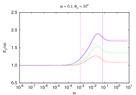
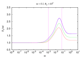
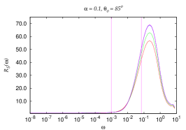
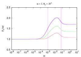
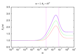
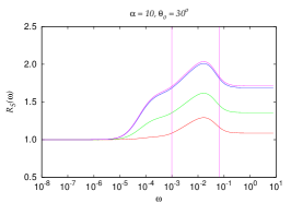
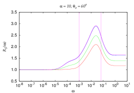
In order to see at which frequencies the relativistic effects are most important, we construct the ratio $R_{\rm{}S}(\omega)$ of the PSD calculated with (denoted by superscript “gr”) and without (“cl”) these effects taken into account:

$$R_{\rm{}S}(\omega)=N_{0}\;\frac{S_{\rm{}P}^{\rm{}gr}(\omega)}{S_{\rm{}P}^{\rm{}cl}(\omega)}\,,$$ (90)

where the normalisation factor is $N_{0}\equiv{S_{\rm{}P}^{\rm{}cl}(0)}/{S_{\rm{}P}^{\rm{}gr}(0)}$. (Doppler and lensing effects are neglected in the calculation of ${S_{\rm{}P}^{\rm{}cl}(\omega)}$.) Figure 9 shows that the PSD graphs are affected only by a constant shift at their low-frequency as well as at the high-frequency limits, i.e., the ratio $R_{\rm{}S}(\omega)$ reaches a constant value at both ends of the frequency range. This is quite easy to understand as at the ends ends of the frequency domain the relativistic PSD acquires the same slope as the non-relativistic one. Relativity shapes the PSD especially within the range of orbital frequencies of the assumed spot distribution.

5 Conclusions

We adopted the viewpoint that the variability pattern is determined by the interplay among the bulk orbital motion, relativistic effects, and the intrinsic changes of the inner accretion disc. We concentrated our attention solely on the PSD characteristics. The spots have a certain kind of memory in our model.

We gave several examples in which the PSD changes the slope and certain break frequencies. The frequency of the break depends on the interplay of model properties, i.e., the intrinsic form of the spot light curves, which determine the individual contributions to the total signal together with the avalanche mechanism. The location of spots on the disc and the inclination of the source define the importance of relativistic effects.

In some cases, a double break occurs and the overall PSD profile is then approximated by a broken power law. This is a promising feature in view of applications to real sources with accreting black holes. The broken power-law profile either resembles a combination of the Lorentzians or, in some cases, an intermediate power law develops and connects the two peaks across the middle frequencies. The change of the PSD slope is clearly visible and well-defined in some cases, though under most circumstances it appears rather blurry. The low-frequency limit of the PSD slope is a constant; the-high frequency behaviour depends mainly on the shape of the spot emission profile, including the general relativity effects. In our calculations the emissivity was decaying exponentially and the slope of the PSD was equal to $-2$ at high frequencies. In between those two limits the intrinsic PSD is influenced by both the individual light curve profile and the underlying process.

It is interesting to notice that the doubly-broken power law occurs only for certain assumptions about the intrinsic light curves of the individual spots or avalanches – their onset and the decay; in other cases the break frequencies are not well defined, or the broken power-law PSD is not preferred at all. We stress that if two Lorentzian seem to dominate the PSD (i.e., two peaks show up), it still does not necessarily mean that two single oscillation mechanisms operate simultaneously. Instead, it may well be the manifestation of the avalanche mechanism.

We employed a general statistical approach to the variability of a black hole accretion disc with orbiting spots that continuously arise and decay. The origin and evolution of spots were described by Poissonian and Hawkes’ processes, the latter one representing a category of avalanche models. We derived analytical formulae for the PSD, Eqs. (14) and (33), and we discussed their limitations and accuracy. The main advantage of the analytical form is the insight into the properties and the fast evaluation that captures the main trends of the PSD shape.

It is worth noting that the PSD does not maintain all information about the light curves that can be studied by Fourier methods (Vio et al. 1992). Extensions have been discussed and compared with real data (Krolik et al. 1993; Karas 1997; Nowak et al. 1999; Vaughan & Uttley 2008), but this would go beyond the scope of our present work.

Our approach allows us to investigate the influence of the assumed mechanism, which describes the creation of parent spots and of subsequent cascades of daughter spots. In particular, we can discuss the PSD slope at different frequency ranges and locate the break frequencies depending on the model parameters. The relationship between the mathematical nature of the process and the PSD of the resulting signal is an interesting consequence of this investigation, as it provides a way to grasp and rigorously constrain the physical models of the source. Therefore we believe that the method that we described is very helpful for identifying the underlying mechanisms that shape the PSD in black hole accreting sources.

Appendix A Spots as a random process

A.1 Assumptions, definitions and preliminaries

In this Appendix, we briefly introduce the formal mathematical approach and notation used throughout the paper. We employ the concept of random values on probability space, $\left(\Omega,\Sigma,P\right)$ (Kolmogorov 1950; Cox & Miller 1965), where $\Omega$ is the sample space (i.e., the set of all possible outcomes of an experiment), $\Sigma$ denotes the $\sigma$-algebra on $\Omega$, and $P$ is non-negative, $\sigma$-additive measure satisfying conditions $P(\emptyset)=0$, $P(\Omega)=1$. It is usually assumed on physical grounds that real signals satisfy all mathematical prerequisites.

A real random value is a map $X$ from $\Omega$ to real numbers, $X:\Omega\rightarrow\mathbb{R}$. The distribution function $F(x)$ and the probability density function $f(x)$ are then defined by

$$F(x)=P\left(\{\varpi\in\Omega\,|\,X(\varpi)<x\}\right),\quad f(x)=\frac{{\rm d}}{{\rm d}x}F(x).$$ (91)

The mean value operator E acts as

$${\rm E}\big{[}g(X)\big{]}=\int\limits_{\mathbb{R}}g(x)\,F({\rm d}x)=\int\limits_{\mathbb{R}}g(x)\,f(x)\,{\rm d}x.$$ (92)

Random values are characterised by their moments, defined as ${\cal M}_{k}\equiv{\rm E}[X^{k}]$. The above-given relations can be generalised to higher dimensions by introducing a $k$-dimensional vectorial random value, $\mbox{\boldmath$X$}=(X_{1},\dots,X_{k})$, the distribution function $F(\mbox{\boldmath$x$})$, and the probability distribution

$$f(\mbox{\boldmath$x$})=\frac{\partial}{\partial x_{1}}\dots\frac{\partial}{\partial x_{k}}F(\mbox{\boldmath$x$}).$$ (93)

From the common distribution, $F(\mbox{\boldmath$x$})$, marginal distributions $F_{i}(x_{i})$ can be derived, as well as the mean value ${\rm E}[h]$ of quantity $h(\mbox{\boldmath$X$})$:

$$F_{i}(x_{i})=\!\!\int\limits_{\mathbb{R}^{k-1}}\!\!\!F\Big{[}\prod\limits_{j\not=i}{\rm d}x_{j}\Big{]},\quad{\rm E}[h]=\!\int\limits_{\mathbb{R}^{k}}\!h(\mbox{\boldmath$x$})\,F\Big{[}\prod\limits_{j=1}^{k}\!{\rm d}x_{j}\Big{]}.$$ (94)

Most important for applications are the first and the second moments, which receive their own designation: $\mu_{i}={\rm E}[X_{i}]$, and $R_{ij}={\rm E}[X_{i}\,X_{j}]$, respectively. The meaning of $R_{ij}$ is the correlation matrix. Finally, it is useful to introduce the covariance matrix,

$$C_{ij}={\rm E}\big{[}X_{i}\,X_{j}\big{]}-{\rm E}\big{[}X_{i}\big{]}\;{\rm E}\big{[}X_{j}\big{]}=R_{ij}-\mu_{i}\,\mu_{j}.$$ (95)

It can be proven that statistically independent random values are always uncorrelated, in which case $C_{ij}$ is a diagonal matrix.

A.2 Random processes

Random processes are a mathematical description of measurements of a physical quantity which is either disturbed by noise or subject to non-deterministic evolution by itself. A random process is a collection of random values $\{X(t):t\in\mathbb{T}\}$ with respect to $(\Omega,\Sigma,P)$, where $\mathbb{T}$ is a time set (usually a subset of $\mathbb{R}$ or a set of integers). For every finite set of points $\{t_{1},\dots,t_{n}\}\subset\mathbb{T}$, one can find the distribution function $F_{t_{1},\dots,t_{n}}(x_{1},\dots,x_{n})$ corresponding to the random vector $\mbox{\boldmath$X$}_{n}=(X(t_{1}),\dots,X(t_{n}))$.

The random process can be interpreted as a function of two variables, $X\equiv X(t,\varpi)$. For a fixed value of some $\varpi^{\prime}\in\Omega$, $X(t,\varpi^{\prime})$ is a function of time, called the trajectory or the realisation of the random process. For a fixed value of $t^{\prime}\in\mathbb{T}$, the function $X(t^{\prime},\varpi)$ is a real random value. A process is called stationary if $F_{t_{1},\dots,t_{n}}(x_{1},\dots,\ x_{n})=F_{t_{1}+r,\dots,t_{n}+r}(x_{1},\dots,x_{n})$ for every $r\in\mathbb{T}$. This implies that all moments of $X(t)$ are independent of time,

$${\rm E}\big{[}X^{k}(t)\big{]}={\rm E}\big{[}X^{k}(t+r)\big{]}={\cal M}_{k},$$ (96)

for all $r$ and $t$. A weaker form of this condition is often used: a random process is called a weak-sense stationary if

$${\rm E}\big{[}X(t)\big{]}={\rm E}\big{[}X(t+r)\big{]},\quad{\rm E}\big{[}X^{2}(t)\big{]}={\rm E}\big{[}X^{2}(t+r)\big{]}.$$ (97)

A stationary random process does not change its nature with time. However, in general there is no way to calculate the statistical characteristics of such a process knowing only a single realisation. For this purpose, a stronger assumption has to be made: a random process is called an ergodic one if for all fixed $r\in\mathbb{T}$ and a real function $h(x)$

$${\rm E}\big{[}h\left(X(r)\right)\big{]}=\lim\limits_{T\rightarrow\infty}\frac{1}{T}\int\limits_{0}^{T}h\left(X(t)\right){\rm d}t.$$ (98)

It is commonly assumed that real processes satisfy this condition.

Stationary processes can be characterised by autocorrelation $R(t)$ and autocovariance $C(t)$ functions,

$$R(t)={\rm E}\big{[}X(r)\,X(r+t)\big{]},\quad C(t)=R(t)-\mu^{2},$$ (99)

which, according to stationarity, are independent of $r$. By setting $r=-t$ we find that $R(t)=R(-t)$.

Another way of characterising processes is by their spectral properties, which are also our main interest in this paper. Power spectral function of a stationary stochastic process $X(t)$ is

$$S(\omega)=\lim\limits_{T\rightarrow\infty}\frac{1}{2T}\;{\rm E}\left[\left|\mathcal{F}_{T}[X(t)](\omega)\right|^{2}\right],$$ (100)

where

$$\mathcal{F}_{T}\big{[}X(t)\big{]}=\int\limits^{T}_{-T}X(t)\,e^{-i\omega t}\,{\rm d}t$$ (101)

is the incomplete Fourier transform. According to the Wiener–Khinchin theorem the power spectral function can be calculated from the autocovariance: $S(\omega)=\mathcal{F}\left[C(t)\right](\omega)$.

A.3 Random point processes

The concept of point processes was originally developed to describe random configurations of points in space (Cox & Miller 1965; Daley & Vere-Jones 2003). One way to characterise such random configurations in some topological space $\mathcal{X}\subset\mathbb{R}^{n}$ is by means of the counting measure, $N(A)$. For every $A\subset\mathcal{X}$, the counting measure gives the number of points lying in $A$.

Similar to random processes, a random point process can be characterised by its mean value and moments. The first-order moment is called the intensity measure,

$$M_{1}(A)={\rm E}\big{[}N(A)\big{]}.$$ (102)

For every $A\subset\mathcal{X}$, $M_{1}(A)$ is the mean number of points in $A$. The second-order moment measure is then

$$M_{2}(A\times B)={\rm E}\big{[}N(A)N(B)\big{]}.$$ (103)

Let $\{x_{i}\}$ be one possible configuration of points, i.e. the support of some $N(.)$. For the functions $h(x)$ and $g(x,y)$ on $\mathcal{X}$ and $\mathcal{X}^{2}$, respectively, it follows (Campbell 1909; Daley & Vere-Jones 2003)

$${\rm E}\Big{[}\!\sum\limits_{i}h(x_{i})\Big{]} = \int\limits_{\mathcal{X}}h(x)\,M_{1}({\rm d}x),$$ (104)

$${\rm E}\Big{[}\!\sum\limits_{i,j}g(x_{i},\,x_{j})\Big{]} = \int\limits_{\mathcal{X}^{2}}g(x,y)\,M_{2}({\rm d}x\times{\rm dy}).$$ (105)

The concept of point process can be further generalised by adding marks, $\kappa_{i}$, from the mark set $\mathcal{K}$ to each coordinate $x_{i}$ from $\{x_{i}\}$. Marks carry additional information (for example, they can be employed to describe the radial distribution of spots and some relations among spots located at different radii; see Sect. 3.2). The resulting point process on the set $\mathcal{X}\times\mathcal{K}$ is called the marked point process if for every $A\subset\mathcal{X}$ it fulfils the condition $N_{\rm g}(A)\equiv N(A\times\mathcal{K})<\infty$.

The random measure $N_{\rm g}(A)$ represents the ground process of the marked process $N$. If the dynamics of the process is governed only by the ground process and the marks are mutually independent and random values with the distribution functions $G({\rm d}\kappa)$, then the measure of the marked process fulfils

$$M_{1}({\rm d}x\!\times\!{\rm d}\kappa)\! = \!M_{{\rm g}1}({\rm d}x)\;G({\rm d}\kappa),$$ (106)

$$M_{2}({\rm d}x_{1}\!\times\!{\rm d}\kappa_{1}\!\times\!{\rm d}x_{2}\!\times\!{\rm d}\kappa_{2})\! = \!M_{{\rm g}2}({\rm d}x_{1}\!\times\!{\rm d}x_{2})\,G({\rm d}\kappa_{1})\,G({\rm d}\kappa_{2}).$$ (107)

Finally, it is useful to introduce the factorial measures, which will be used later to simplify various expressions. They satisfy definitional relations

$$M_{[1]}(A) \equiv M_{1}(A),$$ (108)

$$M_{[2]}(A\times B) \equiv M_{2}(A\times B)-M_{1}(A\cap B).$$ (109)

References

- Abramowicz et al. (1991) Abramowicz, M. A., Bao, G., Lanza, A., & Zhang, X.-H. 1991, A&A, 245, 454
- Blandford et al. (1990) Blandford, R. D., Netzer, H., Woltjer, L., Courvoisier, T. J.-L., & Mayor, M. 1990, Active Galactic Nuclei, Saas-Fee Advanced Course 20 (Springer: Berlin)
- Brémaud & Massoulié (2002) Brémaud, P. & Massoulié, L. 2002, Advances in Applied Probability, 34(1), 205
- Brémaud et al. (2005) Brémaud, P., Massoulié, L., & Ridolfi, A. 2005, Advances in Applied Probability, 37(4), 1116
- Campbell (1909) Campbell, N. R. 1909, Proc. Cambridge Philos. Soc., 15, 117
- Cox & Miller (1965) Cox, D. R. & Miller, H. D. 1965, The Theory of Stochastic Processes (Wiley: New York)
- Czerny et al. (2004) Czerny, B., Różańska, A., Dovčiak, M., Karas, V., & Dumont, A.-M. 2004, A&A, 420, 1
- Daley & Vere-Jones (2003) Daley, D. J. & Vere-Jones, D. 2003, An Introduction to the Theory of Point Processes, Vol. I: Elementary Theory and Methods (Springer: Berlin)
- Dovčiak et al. (2008) Dovčiak, M., Karas, V., Matt, G., & Goosmann, R. W. 2008, MNRAS, 384, 361
- Feigelson & Babu (1992) Feigelson, E. D. & Babu, G. J. 1992, Statistical Challenges in Modern Astronomy (Springer: Berlin)
- Feller (1971) Feller, W. 1971, An Introduction to Probability Theory and Its Applications (New York: Wiley)
- Galeev et al. (1979) Galeev, A. A., Rosner, R., & Vaiana, G. S. 1979, ApJ, 229, 318
- Gardiner (1994) Gardiner, C. W. 1994, Handbook of Stochastic Methods for Physics, Chemistry and the Natural Sciences (Berlin: Springer)
- Gaskell et al. (2006) Gaskell, C. M., McHardy, I. M., Peterson, B. M., & Sergeev, S. G., eds. 2006, Astronomical Society of the Pacific Conf. Series, Vol. 360, AGN Variability from X-Rays to Radio Waves
- Hawkes (1971) Hawkes, A. G. 1971, Biometrica, 58, 83
- Karas (1997) Karas, V. 1997, MNRAS, 288, 12
- Karas et al. (1995) Karas, V., Lanza, A., & Vokrouhlický, D. 1995, ApJ, 440, 108
- Kolmogorov (1950) Kolmogorov, A. N. 1950, Foundations of Probability Theory (Chelsea: New York)
- Krolik et al. (1993) Krolik, J., Done, C., & Madejski, G. 1993, ApJ, 402, 432
- Lawrence & Papadakis (1993) Lawrence, A. & Papadakis, I. 1993, ApJ, 414, L85
- Lawrence et al. (1987) Lawrence, A., Watson, M. G., Pounds, K. A., & Elvis, M. 1987, Nature, 325, 694
- Lehto (1989) Lehto, H. J. 1989, in ESA Special Publication, Vol. 296, Two Topics in X-Ray Astronomy, ed. J. Hunt & B. Battrick, pp. 499–503
- Lyubarskii (1997) Lyubarskii, Y. E. 1997, MNRAS, 292, 679
- Markowitz et al. (2003) Markowitz, A., Edelson, R., Vaughan, S., et al. 2003, ApJ, 593, 96
- McHardy & Czerny (1987) McHardy, I. & Czerny, B. 1987, Nature, 325, 696
- McHardy et al. (2007) McHardy, I. M., Arévalo, P., Uttley, P., et al. 2007, MNRAS, 382, 985
- McHardy et al. (2005) McHardy, I. M., Gunn, K. F., Uttley, P., & Goad, M. R. 2005, MNRAS, 359, 1469
- McHardy et al. (2006) McHardy, I. M., Koerding, E., Knigge, C., Uttley, P., & Fender, R. P. 2006, Nature, 444, 730
- Merloni & Fabian (2001) Merloni, A. & Fabian, A. C. 2001, MNRAS, 328, 958
- Mineshige et al. (1994) Mineshige, S., Ouchi, N. B., & Nishimori, H. 1994, PASJ, 46, 97
- Mirabel & Rodríguez (1998) Mirabel, I. F. & Rodríguez, L. F. 1998, Nature, 392, 673
- Misner et al. (1973) Misner, C. W., Thorne, K. S., & Wheeler, J. A. 1973, Gravitation (W. H. Freeman and Co.: San Francisco, 1973)
- Mushotzky et al. (1993) Mushotzky, R. F., Done, C., & Pounds, K. A. 1993, ARA&A, 31, 717
- Nowak et al. (1999) Nowak, M. A., Vaughan, B. A., Wilms, J., Dove, J. B., & Begelman, M. C. 1999, ApJ, 510, 874
- Pecháček (2008) Pecháček, T. 2008, PhD Thesis (Charles University: Prague)
- Pecháček et al. (2006) Pecháček, T., Dovčiak, M., & Karas, V. 2006, Astronomische Nachrichten, 327, 957
- Pecháček et al. (2005) Pecháček, T., Dovčiak, M., Karas, V., & Matt, G. 2005, A&A, 441, 855
- Pecháček & Karas (2007) Pecháček, T. & Karas, V. 2007, in RAGtime 8/9: Workshops on Black Holes and Neutron Stars, ed. S. Hledík & Z. Stuchlík (Silesian University: Opava), pp. 177–187
- Poutanen & Fabian (1999) Poutanen, J. & Fabian, A. C. 1999, MNRAS, 306, L31
- Stern & Svensson (1996) Stern, B. E. & Svensson, R. 1996, ApJ, 469, L109
- Uttley et al. (2002) Uttley, P., McHardy, I. M., & Papadakis, I. E. 2002, MNRAS, 332, 231
- Vaughan & Uttley (2008) Vaughan, S. & Uttley, P. 2008, in Noise and Fluctuations, Proc. SPIE, Vol. 6603, arXiv:0802.0391
- Vio et al. (1992) Vio, R., Cristiani, S., Lessi, O., & Provenzale, A. 1992, ApJ, 391, 518
- Wiita et al. (1992) Wiita, P. J., Mangalam, A. V., & Chakrabarti, S. K. 1992, in Testing the AGN Paradigm (American Institute of Physics Conf. Series), ed. S. S. Holt, S. G. Neff, & C. M. Urry, Vol. 254, pp. 251–254
- Zhang & Bao (1991) Zhang, X.-H. & Bao, G. 1991, A&A, 246, 21
- Życki (2002) Życki, P. T. 2002, MNRAS, 333, 800
- Życki & Niedźwiecki (2005) Życki, P. T. & Niedźwiecki, A. 2005, MNRAS, 359, 308