The ESO-Spitzer Imaging extragalactic Survey (ESIS) II:
VIMOS I,z wide field imaging of ELAIS-S1 and selection of distant massive galaxies

Abstract

Context. The ESO-Spitzer Imaging extragalactic Survey (ESIS) is the optical follow up of the Spitzer Wide-area Infra-Red Extragalactic survey (SWIRE) in the ELAIS-S1 region of the sky.

Aims. In the era of observational cosmology, the main efforts are focused on the study of galaxy evolution and its environmental dependence. Wide area, multiwavelength, extragalactic surveys are needed in order to probe sufficiently large volumes, minimize cosmic variance and find significant numbers of rare objects.

Methods. We present VIMOS $I$ and $z$ band imaging belonging to the ESIS survey. A total of $\sim 4$ deg² were targeted in $I$ and $\sim 1$ deg² in $z$. Accurate data processing includes removal of fringing, and mosaicking of the complex observing pattern. Completeness levels and photometric uncertainties are estimated through simulations. The multi-wavelength data available in the area are exploited to identify high-redshift galaxies, using the IR-peak technique.

Results. More than 300000 galaxies have been detected in the $I$ band and $\sim 50000$ in the $z$ band. Object coordinates are defined within an uncertainty of $\sim 0.2$ arcsec r.m.s., with respect to GSC 2.2. We reach a 90% average completeness at 23.1 and 22.5 mag (Vega) in the $I$ and $z$ bands, respectively. On the basis of IRAC colors, we identified galaxies having the 1.6$\mu$m stellar peak shifted to $z=1-3$. The new $I,\ z$ band data provide reliable constraints to avoid low-redshift interlopers and reinforce this selection. Roughly 1000 galaxies between $z=2-3$ were identified over the ESIS $\sim 4$ deg², at the SWIRE 5.8$\mu$m depth (25.8 $\mu$Jy at 3$\sigma$). These are the best galaxy candidates to dominate the massive tail ($M>10^{11}$ M_⊙) of the $z>2$ mass function.

1 Introduction

In the recent years, the observational effort in cosmology has focused on the understanding of galaxy formation and tracing the processes that transformed the smooth and homogeneous Universe detected right after the Big Bang into the clumpy, clustered structures we see at $z=0$.

With this respect, the critical parameters to be probed turned out to be baryonic mass and the epoch of its major assembly (e.g. Pozzetti et al. 2007; Rudnick et al. 2006, 2003; Dickinson et al. 2003b; Brinchmann & Ellis 2000). In this respect, particularly controversial is the origin of the recently discovered population of massive ($M>10^{11}$ M_⊙) galaxies at redshift $z>1.5-2.0$ (e.g. Berta et al. 2007a; Fontana et al. 2006, 2004; Franceschini et al. 2006; Bundy et al. 2005; Daddi et al. 2004; Cimatti et al. 2002).

This puzzle has been approached with two opposite “philosophies”: very-deep, pencil-beam surveys, or wide-area, shallower surveys.

The first approach has mostly relied on space-based and 8m telescopes observations, that provided the deepest and clearest views of the distant Universe so far. Some examples, are the Hubble Deep Fields (Williams et al. 1996, 2000), the GOODS survey (Dickinson et al. 2003a) and the Hubble Ultra Deep Field (Beckwith et al. 2003), pushing the detection limit to the 30th magnitude.

Due to their small areas, these surveys are affected by non negligible cosmic variance, which can be a significant source of uncertainty in the study of galaxy statistical properties, even at high redshift (see for example Somerville et al. 2004).

Moreover the search for rare objects, such as massive high-redshift galaxies, requires large volumes to be sampled, in order to detect them in representative numbers. For example, Berta et al. (2007a) find a number density of $\sim 3\times 10^{-5}$ $[$h${}_{70}^{3}$ Mpc${}^{-3}]$ for $M>1.6\times 10^{11}$ M_⊙ galaxies at $z=2-3$, which translates in only a few hundreds sources per square degree.

In overcoming these effects, wide field surveys, such as COSMOS (2 deg² Scoville et al. 2007b), VVDS (16 deg² Le Fèvre et al. 2004), CFHTLS (4 to 410 deg² at different depths, e.g. Nuijten et al. 2005) play a crucial role.

In this framework, the Spitzer Wide-area Infra-Red Extragalactic survey (SWIRE, 49 deg²) is quite unique. The availability of Spitzer IRAC (3.6, 4.5, 5.8, 8.0 $\mu$m) data samples the restframe near-IR emission of galaxies up to redshift $z=3$ at least, directly probing the stellar mass assembly of galaxies in the distant Universe. Despite SWIRE being a rather shallow survey (reaching 5$\sigma$ depths of 3.7 and 43 $\mu$Jy at 3.6 and 5.8 $\mu$m, respectively), it detects $2\times 10^{11}$ M_⊙ galaxies up to $z=3$ (Berta et al. 2007a). MIPS (mainly 24$\mu$m) data secure the identification of star forming systems in the same redshift range.

An extensive multi-wavelength coverage is required. When dealing with large datasets over such a wide area, a spectroscopic characterization of the survey is beyond the multiplexing capabilities of current instrumentation, and photometric investigation is clearly the only viable approach to be carried out in a reasonable amount of time.

The ESO-Spitzer wide-area Imaging Survey (ESIS) is an ESO Large Programme (P.I. Alberto Franceschini), targeting the SWIRE ELAIS-S1 field. This region includes the absolute minimum of the Galactic 100 $\mu$m emission in the Southern sky (0.37 $[$MJy/sr$]$).

In paper-I (Berta et al. 2006) we presented the ESIS WFI/2.2m observations in the $B$, $V$, $R$ bands, illustrating also the potential of panchromatic studies of galaxies. Here VIMOS $I$ and $z$ band observations are presented, completing the optical ESIS survey.

The paper is organized as follows. Section 2 presents the survey and the observing strategy. Section 3 and Appendix A describe the main steps in the data reduction, including astrometric, photometric calibration and mosaicking. The quality of data products is tested in Sect. 4, while the contents of the released catalogs are described in Sect. 5. In Sect. 6 we show how VIMOS $I$ and $z$ band data help in the selection and in constraining the spectral energy distributions (SEDs) of high-redshift galaxies. Finally, Sect. 7 summarizes our findings.

2 Observations

The ESIS VIMOS project covers a total area of $\sim$4 deg² in the $I$ band and $\sim$1 deg² in the $z$ band. A total of 116 hours have been allocated, during periods P71-P73 (from April 2003 to September 2004); observations were carried over also in period P74 (from October 2004 to March 2005).

Figure 1 shows the position of the surveyed area, with respect to other available observations. VIMOS fields are plotted as shaded areas (in blue/dark $I$ band only and in red/light $I+z$ pointings). Multiwavelength imaging includes Spitzer/SWIRE (Lonsdale et al. 2003, 2004), optical ESIS WFI (Berta et al. 2006), near-IR $JK$ (Dias et al. 2007), GALEX (Martin et al. 2005; Burgarella et al. 2005), XMM (Puccetti et al. 2006), Chandra (Feruglio et al., sub.), ELAIS ISO (e.g. Rowan-Robinson et al. 2004), ATCA 1.4 GHz (Middelberg et al. 2007; Gruppioni et al. 1999). See Berta et al. (2006) for a summary and description of all available data. The VIMOS $z$ band observations are centered on the sub-area targeted by X-ray and $JK$ observations.

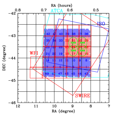
Figure 1: The ESIS VIMOS survey in ELAIS-S1 and the multiwavelength coverage of the area. The shaded area represents the 49 ESIS VIMOS pointings in the $I$ (blue/dark) and $I+z$ (red/light) bands. Over plotted are: the ESIS WFI survey ($\sim 30^{\prime}\times 30^{\prime}$ squares Berta et al. 2006) and the SWIRE (Lonsdale et al. 2003, 2004), XMM (Puccetti et al. 2006), ELAIS ISO (e.g. Rowan-Robinson et al. 2004), ATCA 1.4 GHz (Middelberg et al. 2007; Gruppioni et al. 1999) areas.

The VIMOS (LeFevre et al. 2003) array is made of 4 CCDs, each one covering $\sim 6.5^{\prime}\times 8^{\prime}$ in the sky, separated by large gaps ($\sim 120-140$ arcsec wide, depending of which CCDs are considered). The pixel scale is 0.205 arcsec/pixel.

In order to cover a contiguous area and minimize overheads, the observing strategy was set as follows:

1. the total area is divided into 37 $I$ and 12 $I+z$ pointings (see Fig. 1).

2. each pointing is effectively made of 3 different Observing Blocks (OBs), named “A, B, C”. Between pointings A and B one-gap-wide x,y offsets exist; the same holds between B and C pointings (see Fig. 2, left panel).

3. each one of these 3 OBs is made of 4 dithered exposures, in order to get rid of bad pixels and gap signatures (see Fig. 2, right panel).

4. care has been taken in order to observe at least one of the 3 OBs per pointing during a photometric night. In this way, it is possible to compute photometric offsets and correct the whole field to photometric conditions.

5. the total number of individual science exposures is 588 and 144 in the $I$ and $z$ band respectively.

6. the total exposure time per OB is 600s in the $I$ band and 1200s in the $z$ band, causing saturation at $I\sim 16$ $[$Vega$]$.

7. as a result of offsetting (3 OBs per pointing), the final coverage is not homogeneous, but there are regions with a 600s coverage, others with 1200s (the majority) and finally some with 1800s coverage. These values refer to the $I$ band; as far as the $z$ band is concerned, the effective exposure times are 1200s, 2400s, 3600s.

Figure 3 shows the average VIMOS $I$ and $z$ passbands, defined as filters convolved with CCD and optics response. Actually the VIMOS transmission depends slightly on which of the four quadrants is considered. Here here we adopt an average transmission. Tables 4 and 5 (available in electronic version) list the observation logs of the ESIS VIMOS survey.

Figure 2: Scheme of the ESIS VIMOS observing strategy. Left panel: each pointing is made of three different OBs, shifted in the sky in order to fill gaps between CCDs. Right panel: each OB consist of four dithered exposures, for optimal bad pixels masking.

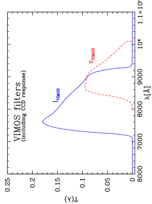
Figure 3: The VIMOS $I$ and $z$ passbands average transmissivity.

3 Data reduction

The ESIS VIMOS data were reduced within the IRAF environment, exploiting the capabilities of the WFPDRED package, developed in Padova and adapted to the VIMOS case.

De-biasing and flat-fielding were performed in the standard manner; sky flat field frames taken during each night were used. VIMOS $I$ and $z$ band images are affected by strong fringing, that needs to be corrected before photometric calibration and mosaicking. Appendix A describes the main causes of fringing and the procedure adopted to correct ESIS frames. Figure 4 shows one VIMOS $I$ band frame before (left panel) and after (right panel) subtracting the fringe pattern (central panel).

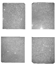
(a) Image before de-fringing

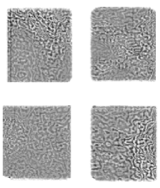
(b) Fringe pattern

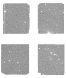
(c) Image after de-fringing

Figure 4: Example of de-fringing process in the $I$ band.

3.1 Astrometric calibration

The ESIS survey targets a large area in the sky ($\sim$4 deg² in the $I$ band), therefore it is necessary to accurately map the astrometric distortion of VIMOS, in order to correctly build wide-field mosaics.

The survey includes observations of the Stone et al. (1999) astrometric fields D and E, obtained both with the WFI and VIMOS instruments, and aimed at properly mapping pixel into celestial coordinates.

We have chosen a TNX mapping (see Berta et al. 2006), which combines a linear projection of the sky sphere onto a tangent plane and a polynomial function for distortions. In order to obtain the best pixels-sky mapping, we have exploited the VIMOS astrometric observations and extended the resulting catalog with the WFI observations.

The best results were obtained using 5th order distortion polynomials. Before mosaicking, the astrometric solution was applied to individual science images, and each frame was re-centered on the GSC 2.2 (STScI & OaTO, 2001) catalog. Section 4.1 reports on the accuracy of ESIS VIMOS astrometry.

3.2 Photometric zeropoints

As part of the ESIS VIMOS observations, Landolt (1992) Ru149 or TPHE spectrophotometric standard fields were targeted during photometric nights, in order to perform a dedicated photometric calibration of ESIS science frames. These observation have been defined with four different exposures per observing block, including the main standard stars on each individual CCD of the VIMOS array.

Unfortunately, these fields are not rich in stars and the VIMOS chips are relatively small, therefore only few objects fall on the CCD, and the estimate of the zeropoints is not optimal. Nevertheless, after the reduction of standard fields and correction of single CCD frames for differences in gain, the $I$ band zeropoints were computed. The resulting zeropoint $zp_{I}=26.96\pm 0.07$ (in units of electrons) is consistent with the ESO value (26.99 on average), computed on richer fields.

As far as the $z$ band is concerned, despite the fact that ESIS included observations of Landolt (1992) fields, no reference standard catalog is available in these fields, therefore we relied on a different procedure to determine the zeropoint.

The ELAIS-S1 field benefits from an extensive multiwavelength follow up from the X-rays to the radio (see Berta et al. 2006). We have therefore selected stars with available BVRJK+IRAC photometry in the ESIS field and performed SED fitting to estimate the expected $z$ band magnitudes and determine the VIMOS zeropoint:

$$ZP=m_{expected}-m_{measured}\textrm{.}$$ (1)

Source extraction has been performed with SExtractor (Bertin & Arnouts 1996) on individual science frames observed during photometric nights and reduced as described above. Each image was transformed into e^-/s, by using the proper gain for the given CCD.

Point-like objects were selected on the basis of the dependence of their half-flux radius on instrumental magnitude (see Fig. 5, bottom left panel, and Sect. 5). This procedure has the advantage of well identifying the magnitude range over which point-like sources are well defined.

The $z$ band extracted catalog was matched to the other wavelengths source lists with a simple closest-neighbor algorithm, using a 1 arcsec matching radius (Berta et al. 2006). The final catalog contains $\sim$50-100 objects per CCD. Since we are using a sub-area of the entire ESIS VIMOS survey (i.e. the region in the sky actually covered by JK data), these photometric images were taken during two epochs only, namely December 2003 and Aug.-Sept. 2004.

The adopted stellar library is based on Pickles (1998) stellar spectra, extended to $\lambda>2.5\mu$m with a Rayleigh-Jeans law.

The observed spectral energy distributions (SEDs) of stellar objects were fitted taking into account optical and near-IR photometry up to the IRAC 4.5$\mu$m band. Best fit is sought by means of $\chi^{2}$ minimization, among all templates in the stellar library and varying their normalization. Two examples of SED fits are shown in Fig. 5. The 5.8$\mu$m flux is also shown (when available), even if it was not included in the estimation of $\chi^{2}$. The 1,2,3 $\sigma$ uncertainty on the expected $z$ band magnitude, as derived from the best fit, is computed as $\chi_{best}^{2}+1,4,9$.

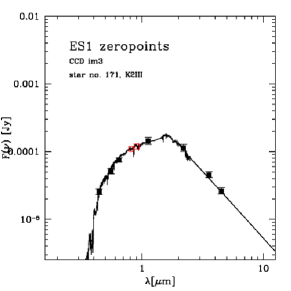
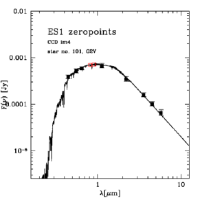
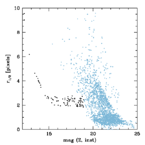
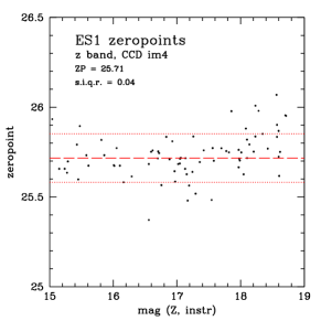
Figure 5: Determination of VIMOS zeropoints. Top panels: two examples of SED fitting of stars in ESIS photometric pointings. The open squares represent the $I$ and $z$ band expected fluxes derived from the best fit. Bottom left panel: selection of point-like objects on the $z$ band photometric images used to derive zeropoints. The dark dots represent the “stellar” locus. Bottom right panel: $z$ band zeropoint for CCD 4. The dashed line represents the median, the dotted lines are the $\pm 3\ s.i.q.r.$ levels used for clipping the data.

The zeropoint for a given CCD is given by the median of all zeropoints (one per star, see Fig. 5). We used a 3 s.i.q.r. clipping (corresponding to a 2 $\sigma$ clipping for a normal distribution).

As zeropoint differences between different chips are mainly due to gain differences, the resulting zeropoints for the 4 VIMOS quadrants are consistent with each other. The $z$ band zeropoint obtained in this way is (in units of electrons):

$$ZP(Z\ \textrm{band})=25.74\pm 0.11$$ (2)

where the uncertainty is given by $4\times s.i.q.r.$.

Similarly, we have taken advantage of the selected stellar catalogs to newly compute the zeropoint in the $I$ band, directly from ESIS data, obtaining a zeropoint of $26.93\pm 0.13$ mag (in units of electrons), consistent with our previous and ESO’s estimates. No significant difference in zeropoints between the two epochs is detected.

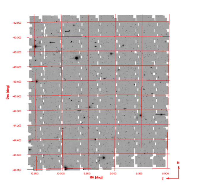
Figure 6: The ESIS VIMOS final $I$ band mosaic.

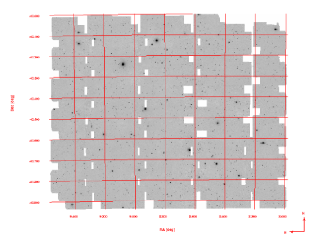
Figure 7: The ESIS VIMOS final $z$ band mosaic.

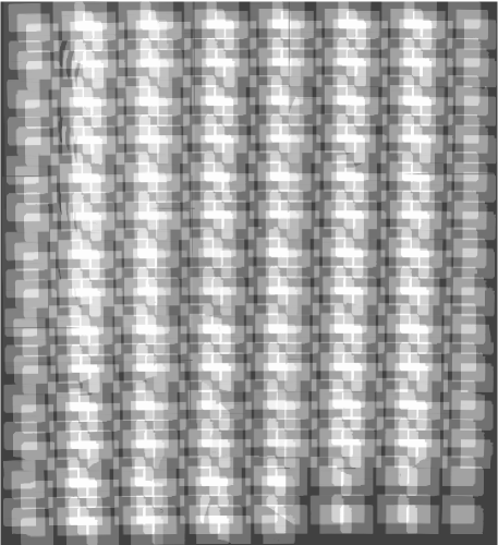
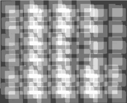
Figure 8: The ESIS VIMOS final $I$ (left) and $z$ band (right) exposure maps. Brighter regions correspond to deeper coverage. North is up, east is left; the two images have roughly the same scale.

3.3 Photometric calibration

As already pointed out, the observations of ESIS VIMOS fields are spread across several nights, and are characterized by different sky conditions.

The requirement that at least one OB per pointing was observed in photometric conditions facilitates the task of absolute calibration of the whole dataset; we call these photometric images “reference frames”. We have identified point-like objects on each science image, in common with any reference frame and then computed the zeropoint shift due to non-photometric conditions: $\Delta mag=mag_{any}-mag_{ref}$.

Hence, each individual frame has been corrected to photometric conditions, normalized to unitary airmass and exposure time, and converted to electrons:

$$I_{phot}=\frac{I_{any}\times 10^{0.4\left(AM\cdot K_{\lambda}+\Delta mag\right)}}{t_{exp}}\times\textrm{\em CONAD}\textrm{,}$$ (3)

where AM is the airmass of the given frame, $K_{\lambda}$ is the atmospheric extinction coefficient for Paranal ($K_{I}=0.027$, $K_{z}=0.02$), and CONAD is the gain in e^-/ADU.

No color corrections are applied, and final catalogs are given in calibrated VIMOS magnitudes (i.e. not transformed to any standard photometric system). The effective wavelengths for the $I$ and $z$ passbands are 8140 and 9050 Å respectively. The flux zeropoints and AB shifts for these magnitudes are:

$$S(I,\ Jy) = 2385\times 10^{0.4\cdot mag(I,\ Vega)}$$ (4)

$$S(z,\ Jy) = 2207\times 10^{0.4\cdot mag(z,\ Vega)}$$ (5)

$$mag(I,\ AB) = mag(I,\ Vega)+0.4763$$ (6)

$$mag(z,\ AB) = mag(z,\ Vega)+0.5604$$ (7)

as derived convolving the spectrum of Vega with VIMOS passbands (see Fig. 3).

3.4 Mosaicking

The astrometrically- and photometrically-calibrated frames were finally combined together into the final ESIS mosaics.

In the $I$ band due to the large surveyed area and due to image size limitations, nine different mosaics were produced, in a $3\times 3$ pattern covering the whole ESIS-VIMOS field. For the $z$ band it was possible to assemble one single final mosaic, $\sim 1$ deg² wide.

During co-addition, all frames belonging to a given mosaic were registered to the same astrometric map. Different mosaics have different astrometric maps, using the mosaic center as tangent point for re-projection. Bad pixels and “defects” (e.g. optical reflections or crossing of satellites, see the top panels in Fig. 9) were masked and excluded from the final mosaics.

Because of the complex observing strategy, the effective exposure time varies across the field: the majority of the area has a 75% depth, and smaller regions with 25, 50 and 100% depths exist. We have therefore built weight maps to be associated with each scientific image during catalog extraction. We also include a coverage flag in the extracted catalogs, describing the actual depth at the position of the detected objects.

The entire $I$ band field is shown in Fig. 6, where we have scaled down and combined the 9 sub-areas, for display purposes only. The $z$ band mosaic is in Fig. 7. Figure 8 includes exposure maps. Unfortunately gaps in RA between different pointings are left. This problem is mainly caused by shadowing of the E-W edges of VIMOS CCDs in ESIS images (see the bottom left panel in Fig. 9). The width of the shade varies from frame to frame, and consequently so does the width of the residual gap in the final mosaics. Note that this is different from shadowing by the guiding star probe (bottom right panel). The actual reason for this loss of pixels is not clear.

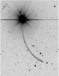
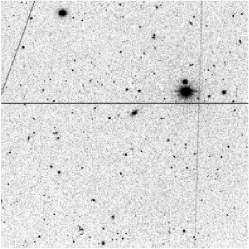
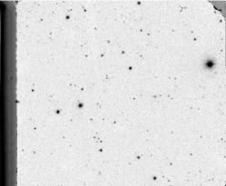
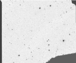
Figure 9: Examples of defects to be masked before mosaicking. Top panels show emission features: optical reflections and satellite trails. Bottom panels exemplify “vignetting” features: the unidentified shade causing residual gaps in the final mosaics (left) and the shadow of the guide star probe (right). For clarity sake we have inverted colors of the shades. North is up, east is left.

4 Quality of data products

Observations were carried out under very different atmospheric conditions, over a $\sim 2$ years period of time. The gaussian FWHM of point-like sources is therefore not constant across the ESIS field, but there are regions with seeing $<0.8$ arcsec and others with $\textrm{FWHM}\mathrel{\hbox{\hbox to0.0pt{\hbox{\lower 4.0pt\hbox{$\sim$}}\hss}\hbox{$>$}}}1.0$ arcsec. The final catalogs were extracted on the mosaics without smoothing to the worst seeing in the field, in order to take advantage of good imaging quality, where available.

We have tested how many sources would be lost by degrading the images with good seeing to a 1 arcsec FWHM PSF, by convolving all individual frames with the appropriate kernel. As a result, roughly 4-5% of the sources is lost when smoothing the images, mainly at the faintest magnitudes, after the turnover in the number counts (see Sect. 5).

Figure 10 shows the trend of seeing as a function of magnitude (left panels). The large scatter reflects what mentioned above. The deviation at bright magnitudes is due to incoming saturation effects. The saturation thresholds for the ESIS VIMOS survey turn out to be $I\sim 16.5$ and $z\sim 16$ mag $[$Vega$]$, consistent with the expectations of ESO’s exposure time calculator ($I\sim 16.2$ and $z\sim 15.8$ for a point-like source with $1{\arcsec}$ seeing and $\textrm{A.M.}=1.3$).

The right hand panels of Fig. 10 illustrate the distribution of seeing across the field. Pointlike sources are plotted in different grey levels (darker indicating better seeing) and dot dimensions (smaller for better FWHM). Three bins are considered: $\textrm{FWHM}\leq 0.8$, $0.8<\textrm{FWHM}\leq 1.0$, $1.0<\textrm{FWHM}\leq 1.2$.

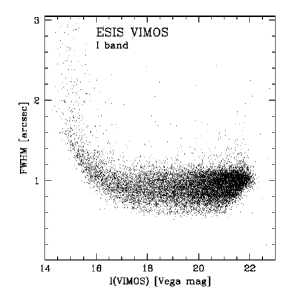
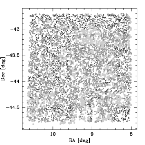
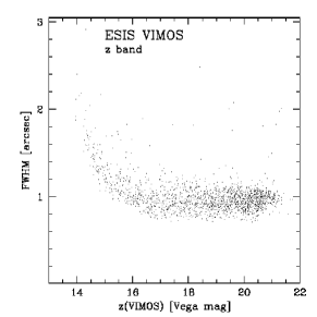
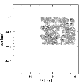
Figure 10: Actual FWHM of pointlike sources in the ESIS VIMOS $I$ band (top panels) and $z$ band (bottom panels) survey. The dependence on magnitude and the variation of FWHM across the field are shown. Grey levels and dot dimensions illustrate seeing properties, darker and smaller dots referring to better FWHM. Three bins are considered: $\textrm{FWHM}\leq 0.8$, $0.8<\textrm{FWHM}\leq 1.0$, $1.0<\textrm{FWHM}\leq 1.2$.

4.1 Astrometric accuracy

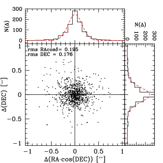
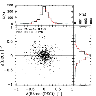
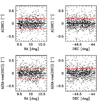
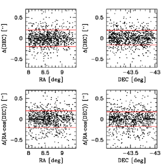
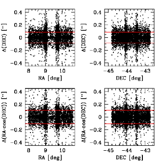
Figure 11: Astrometric accuracy of the ESIS VIMOS survey. Left panels: $I$ band. The top and central plots show the displacement of ESIS coordinates with respect to the GSC 2.2 (STScI & OaTO, 2001) catalog. The bottom figure shows the relative astrometric accuracy between the 9 different $I$ band sub-areas. Right panels: same plots for the $z$ band. Only absolute astrometry is shown, because the $z$ band covers 1 deg² and consists of one single final mosaic. Horizontal solid lines set the $\pm 1\sigma$ levels of $\Delta(coords)$.

The coordinates of the objects detected on the final mosaics have been compared to GSC 2.2 (STScI & OaTO, 2001) sources, after re-centering the GSC catalog on the ESIS images. Figure 11 shows the results for one of the $I$ band mosaics (left panels) and the $z$ band final image (right panels). The r.m.s. of the distribution of coordinate differences for the $I$ and $z$ bands is 0.195 and 0.199 arcsec in $\Delta(RA\cdot\cos[Dec])$ and 0.176 arcsec in $\Delta(Dec)$.

In the central panels in Fig. 11 the coordinate differences between the ESIS and GSC catalogs are plotted against RA and Dec: no systematic trends are detected.

As far as the $I$ band is concerned, we have checked also the coordinate match between the 9 different mosaics, analyzing the differences in (RA,Dec) for GSC sources in the overlap regions (left bottom panel in Fig. 11). The r.m.s. of the distribution of coordinate differences are 0.105 and 0.087 arcsec in $\Delta(RA\cdot\cos[Dec])$ and $\Delta(Dec)$ respectively.

4.2 Photometric accuracy

The photometric accuracy of the data has been tested with simulations, adding synthetic sources to the ESIS final mosaics (with IRAF), adopting a $1{\arcsec}$ seeing, and performing source extraction as for science data.

In each band, we produced several simulated images, by adding point-like, De Vaucouleurs or exponential disk objects at random positions on the science frames. In each case, a different image was produced per 0.25 mag bin, in the range 18-27 mag. A population of $\sim 8000$ sources/deg² was added each time.

Figure 12 compares the input magnitudes of the simulated point-like sources and the values measured by SExtractor. For each of the two bands, the four panels refer to regions in the mosaics having effective depths $<50$%, $50-75$% and $\geq 75$% (see Sect. 5). The solid lines represent the median differences, the short-dashed lines are the 1-$\sigma$ standard deviation and the long-dashed lines trace the semi-inter-quartile ranges (s.i.q.r.). Typical s.i.q.r. uncertainties at $\textrm{mag}=21.5,\ 23.5$ (Vega) are $\sim 0.05,\ 0.20$ in the $I$ band and $\sim 0.08,\ 0.22$ in the $z$ band, on average on the whole area.

Slightly larger uncertainties are found for De Vaucouleurs profiles and exponential disks: the corresponding s.i.q.r. are $\sim 0.07,\ 0.22$ at $\textrm{mag}=21.5,\ 23.5$ (Vega) in the $I$ band and $\sim 0.10,\ 0.27$ in $z$. The usual systematic offset for the recovered magnitudes of De Vaucouleurs objects is present. Its value is $\sim 0.2-0.3$ magnitudes. This offset is well described in the literature (e.g. Fasano et al. 1998): it is due to missing flux in the outskirts of De Vaucouleurs profiles and does not depend on the adopted source extraction code.

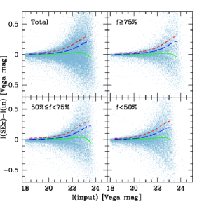
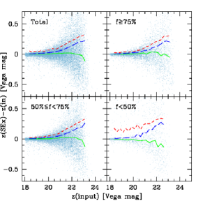
Figure 12: Photometric accuracy, derived by extracting synthetic point-like sources from ESIS VIMOS $I$ band (left) and $z$ band (right) mosaics. Different panels refer to different effective depths. Solid, short-dashed and long-dashed lines trace the median, the 1-$\sigma$ and the s.i.q.r. levels respectively.

4.3 Completeness

By comparing the numbers of input and detected sources in simulations, we derive the detection rate in the ESIS VIMOS survey.

Figure 13 shows the results for point-like sources in the $I$ (left) and $z$ (right) bands, split by coverage again. The vertical dotted lines set the 90% and 95% completeness levels.

On average, the 90% level is reached at magnitude 23.1 and 22.5 (Vega) in the $I$ and $z$ band respectively. These values increase to 23.6 and 23.0, if only the regions with coverage $\geq 75$% are taken into account.

As far as exponential disks and De Vaucouleurs profiles are concerned, the 90% detection rate is shifted to $\sim 0.3$ and $\sim 0.5$ brighter magnitudes levels, respectively.

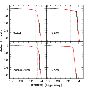
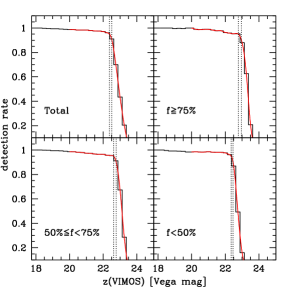
Figure 13: Detection rate as a function of magnitude, from simultaed point-like sources. The vertical dotted lines set the 90% and 95% completeness levels.

Column			Name	Description	Units
	1		ID	ESIS ID
	2		RA	Right Ascension (J2000)	[deg]
	3		DEC	Declination (J2000)	[deg]
	4		MAG_BEST	Best of MAG_AUTO and MAG_ISOCOR	[mag]
	5		MAGERR_BEST	RMS error for MAG_BEST	[mag]
	6		MAG_AUTO	Kron-like elliptical aperture magnitude	[mag]
	7		MAGERR_AUTO	RMS error for Kron-like magnitude	[mag]
	8		MAG_ISOCOR	Corrected isophotal magnitude	[mag]
	9		MAGERR_ISOCOR	RMS error for corrected isophotal magnitude	[mag]
	10		MAG_APER1	Aperture magnitude (1.230 arcsec diam.)	[mag]
	11		MAG_APER2	Aperture magnitude (2.460 arcsec diam.)	[mag]
	12		MAG_APER3	Aperture magnitude (3.280 arcsec diam.)	[mag]
	13		MAG_APER4	Aperture magnitude (4.715 arcsec diam.)	[mag]
	14		MAG_APER5	Aperture magnitude (6.675 arcsec diam.)	[mag]
	15		MAGERR_APER1	RMS error for APER1 magnitude	[mag]
	16		MAGERR_APER2	RMS error for APER2 magnitude	[mag]
	17		MAGERR_APER3	RMS error for APER3 magnitude	[mag]
	18		MAGERR_APER4	RMS error for APER4 magnitude	[mag]
	19		MAGERR_APER5	RMS error for APER5 magnitude	[mag]
	20		SN	Local S/N ratio
	21		KRON_RADIUS	Kron aperture in units of A or B
	22		FWHM_IMAGE	FWHM assuming a gaussian core	[pixel]
	23		CLASS_STAR	Star/Galaxy classifier output
	24		FLUX_RADIUS	Half-flux radius	[pixel]
	25		FLAGS	SExtractor extraction flags
	26		IMAFLAGS_ISO	Coverage flag

Table 1: Contents of ESIS VIMOS $I$ and $z$ band catalogs.

	$I$ band		$z$ band
mag.	$\log N$		$\log N$
$[$Vega$]$	Tot.	Ext.	Tot.	Ext.
14.0	1.915	0.711	1.991	0.610
14.5	2.164	1.267	2.343	1.087
15.0	2.390	1.410	2.388	1.724
15.5	2.497	1.736	2.565	2.254
16.0	2.526	1.736	2.579	2.223
16.5	2.655	2.069	2.656	2.366
17.0	2.738	2.216	2.792	2.597
17.5	2.870	2.430	2.964	2.750
18.0	3.024	2.675	3.113	2.937
18.5	3.181	2.945	3.261	3.143
19.0	3.361	3.188	3.437	3.357
19.5	3.513	3.409	3.580	3.536
20.0	3.659	3.623	3.709	3.687
20.5	3.795	3.788	3.891	3.888
21.0	3.938	3.938	4.017	4.017
21.5	4.087	4.087	4.135	4.135
22.0	4.216	4.216	4.232	4.232
22.5	4.338	4.338	4.264	4.264
23.0	4.410	4.410	4.180	4.180
23.5	4.409	4.409	3.951	3.951
24.0	4.270	4.270	3.433	3.433
24.5	3.901	3.901	–	–
25.0	3.008	3.008	–	–

Table 2: ESIS VIMOS $I$ and $z$ band number counts in units of $[$deg^-2 mag${}^{-1}]$. No completeness correction was applied.

5 Catalogs

The total exact area covered by the $I$ band mosaics is 4.11 deg². Excluding the gaps and areas around very bright stars, the catalog covers 3.89 deg². We define the coverage flag as the fraction $f$ of nominal exposure time (900s for the $I$ band, 1800s in $z$) spent on source; 25%, 64% and 96% of the sources in the $I$ band catalog lie in regions with $f>0.75,\ 0.50,\ 0.25$ respectively.

The $z$ band survey includes a 1.08 deg² area. After removal of regions not covered and big stars, the catalog includes 0.98 deg², 20%, 55% and 96% of which are above $f>0.75,\ 0.50,\ 0.25$.

Catalogs were extracted using SExtractor (Bertin & Arnouts 1996) from the final mosaics, weighting the data with coverage maps. A total of 312929 and 57926 sources were measured in the $I$ and $z$ band respectively.

The list and description of columns included in the released catalogs are provided in Tab. 1. All magnitudes are given in Vega units. Data are provided as electronic tables associated to this work.

Figures 14 shows the ESIS VIMOS number counts, as split by effective depth (top panels) and into point-like and extended sources (bottom panels). The latter are compared to data from the COSMOS (Scoville et al. 2007a; Taniguchi et al. 2007), GOODS-N (Capak et al. 2004), VVDS (McCracken et al. 2003), HDFN, HDFS, William Herschel (WHDF Metcalfe et al. 2001) and SDSS(Yasuda et al. 2001) surveys. The ESIS data are fairly consistent with the literature; discrepancies can be due to cosmic variance at the bright magnitudes, to a different criterion in galaxy/point-like sources separation at intermediate fluxes, and to incoming ESIS incompleteness at the faint end. We warn also that saturation effects might play a role at the brightest fluxes (see Sect. 4).

The data collected from the literature used the SExtractor’s stellarity flag to distinguish these two classes, while here the half-flux radius is exploited (see for example Berta et al. 2006). Figure 15 shows the different selection of point-like objects for the $z$ band, based on a simple cut in the stellarity flag ($>0.95$ in this case, right panel) or based on the dependence of the half-flux radius on magnitude (left panel). Note again the effects of pixel saturation: the bright point-like objects deviate from the locus defined by half-flux radius. The SExtractor stellarity flag misses the brightest saturated point-like sources and tends to be contaminated by galaxies at intermediate fluxes (see also Berta et al. 2006).

Table 2 reports the observed number counts of the ESIS VIMOS survey.

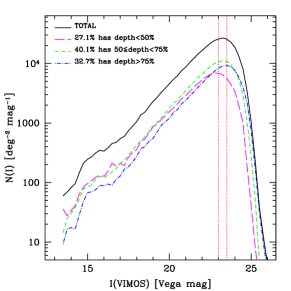
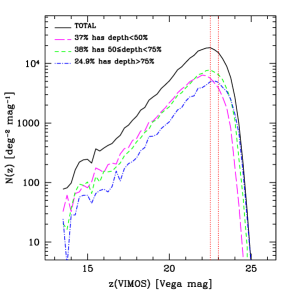
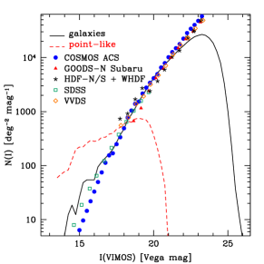
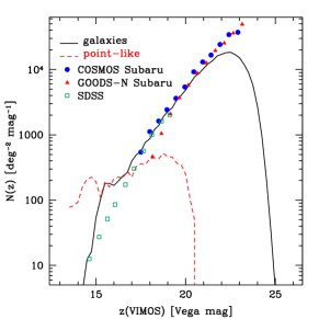
Figure 14: Observed source number counts for the ESIS VIMOS survey, split into effective depth bins (top panels) and into point-like vs. extended sources (bottom panels). Literature data belong to: COSMOS (Scoville et al. 2007a; Taniguchi et al. 2007), GOODS-N (Capak et al. 2004), VVDS (McCracken et al. 2003), HDFN, HDFS, William Herschel (WHDF Metcalfe et al. 2001), SDSS (Yasuda et al. 2001).

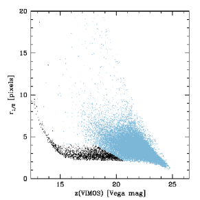
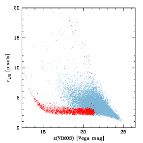
Figure 15: Selection of point-like sources based on the half-flux radius or SExtractor’s stellarity flag (right-hand panel), for the $z$ band. Darker dots represent point-like objects.

6 High-redshift galaxies

Large area, multiwavelength extragalactic surveys are designed to study the evolution of galaxies across cosmic time. SWIRE-ESIS covers the whole electromagnetic spectrum from the X-rays to radio wavelengths and is well suited to identify large samples of any class of objects reachable at its depth.

Of particular interest is the recently discovered class of massive galaxies ($M>10^{11}$ M_⊙) above redshift $z>1.5$, whose formation and evolution appears to be faster than what predicted by pure hierarchical scenarios and apparently showing downsizing effects (e.g. Cimatti et al. 2002; Daddi et al. 2004; Fontana et al. 2006; Bundy et al. 2005; Franceschini et al. 2006).

Thanks to IRAC observations, SWIRE-ESIS directly probes the assembled stellar mass of galaxies up to redshift $z\sim 3$. Due to its moderate depth, SWIRE can detect only the most massive tail of the high-redshift galaxy stellar mass function (e.g. $M>2\times 10^{11}$ M_⊙ at $z\sim 3$, Berta et al. 2007a).

Here we describe how the availability of $I$ and $z$ band data, when combined with the other multiwavelength observations, provides good constraints in the selection of high-$z$ massive galaxies.

For the current purpose, we have matched the SWIRE Spitzer catalog (Lonsdale et al. 2003, 2004) to ESIS $B,\ V,\ R,\ I$ and $z$ (Berta et al. 2006, and this work), near-IR $J$, $K_{s}$ (Dias et al. 2007), and GALEX GR4 data, using a closest neighbor criterion with a 1 arcsec radius (see Berta et al. 2006). We use total magnitudes in all bands. The SWIRE 3$\sigma$ depths are 2.2, 3.2, 25.8, 22.6, 200 $\mu$Jy at 3.6, 4.5, 5.8, 8.0 and 24 $\mu$m; the ESIS BVR 95% completeness levels are reached at magnitudes $B\,V\sim 25$ and $R\sim 24.5$ (Vega); the $J,\ K_{s}$ catalogs are 95% complete at 19.82, 18.73 mag (Vega) respectively.

The ESIS VIMOS $I$ band area includes 219877 SWIRE sources, detected in at least one IRAC band. Among these, 142776 (65%) have at least one optical detection (BVRIz), 137206 are detected in the $I$ band, 52620 in BVR (one band at least, over 1.5 deg²), 35670 in $z$ (over $\sim 1$ deg²), and 30355 are detected in the GALEX DR4 ELAIS-S1 survey. The $z$ band area, covered by all bands (BVRIz, JK_s, Spitzer, GALEX, X-rays and radio), includes 63770 SWIRE sources, 45873 ($\sim 72$%) of which detected in at least one optical band. Table 3 summarizes these statistics.

Class	area	number
	$[$deg${}^{2}]$
SWIRE ($I$-band area)	4.11	219877
SWIRE+BVRIz (one band)	3.89	142776
SWIRE+BVR (one band)	1.5	52620
SWIRE+$I$	3.89	137206
SWIRE+$z$	0.98	35670
SWIRE+GALEX	4.11	30355
24$\mu$m	4.11	12770
SWIRE ($z$-band area)	0.98	63770
SWIRE+BVRIz (one band)	0.98	45873
SWIRE+BVR (one band)	0.98	39883
SWIRE+$I$	0.98	41337
SWIRE+$z$	0.98	35670
SWIRE+GALEX	0.98	8884
24$\mu$m	0.98	3733
4.5$\mu$m-peak (total)	4.11	938
4.5$\mu$m-peak (interlopers)	4.11	353
5.8$\mu$m-peak	4.11	973

Table 3: Multi-wavelength detection statistics in the ELAIS-S1 area.

6.1 Selection of IR-peakers

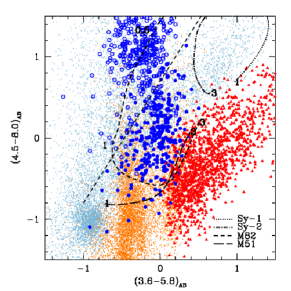
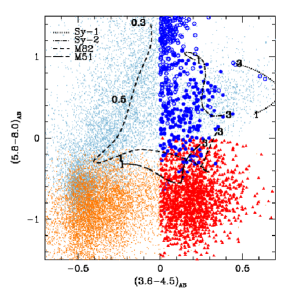
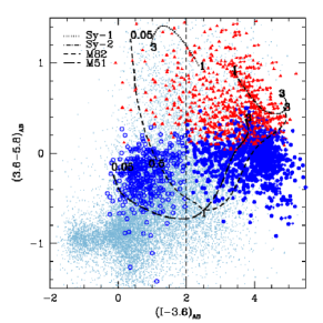
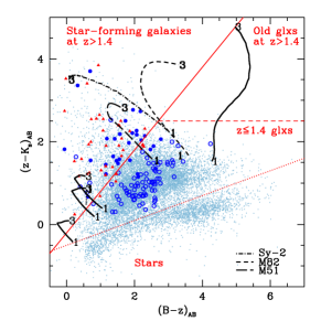
Figure 16: Color-color plots adopted in the selection of IR-peakers. Filled triangles and circles represent 5.8$\mu$m-peakers and 4.5$\mu$m-peakers respectively. Open circles are 4.5$\mu$m-peakers identified as low-redshift interlopers on the basis of $(I-3.6)_{AB}$. Small dots trace the general SWIRE-ESIS population; orange dots are general sources with no 8.0$\mu$m detection (upper limits are used). Redshift tracks for different templates are plotted: M82 (dusty starburst) and M51 (spiral) belong to the GraSil library (Silva et al. 1998); the Sy1 and Sy2 templates represent Mrk231 and IRAS19254-7245 (Fritz et al. 2006; Berta et al. 2003). The black thick solid lines in the $BzK$ diagram (bottom-right panel) represent three GraSil spiral models with no extinction (ages 0.2, 1.0, 2.0 Gyr) and one GraSil elliptical (age 3 Gyr). Redshift values are reported along tracks. The diagonal and vertical dashed lines in the left-hand diagrams represent the color conditions to identify low-redshift interlopers (see text).

Several selection criteria have been defined to identify high redshift galaxies, exploiting optical and near-IR colors (e.g. Ly-break galaxies, LBGs, Steidel et al. 1996, 1999; BX-BM, Adelberger et al. 2004; distant red galaxies, DRGs, Franx et al. 2003; extremely red objects, EROs, Cimatti et al. 2002; distant obscured galaxies, DOGs, Dey et al. 2008; $BzK$, Daddi et al. 2004). LBGs, BX-BM’s and DOGs classes consist of very faint objects that require $U$-band and/or deeper optical observations than those available in the ELAIS-S1 field. EROs and DRGs in ELAIS-S1 are being discussed in a forthcoming paper by Dias et al. (2008, in prep.).

Recently, Berta et al. (2007a) and Lonsdale et al. (2006) have shown that IRAC data allow the selection of high-$z$ (massive) galaxies by identifying the restframe 1.6$\mu$m stellar peak (Sawicki 2002; Simpson & Eisenhardt 1999) in the SEDs of galaxies, redshifted to $z=1.5-3.0$. We called these objects IR-peakers (informally known also as “IR-bump galaxies”).

Berta et al. (2007a) have presented the selection of IR-peakers and studied their stellar content. Here we refine and reinforce the selection using $I$ band data. This allows us not only to avoid low-redshift interlopers, but also to extend the search for these sources over the whole ESIS-VIMOS area ($\sim 4$ deg²), instead of restricting it to the central square degree where optical BVR imaging is available to date.

The main IR-peak selection is based in the detection of the 1.6$\mu$m peak in the IRAC domain. Two different classes of galaxies are identified, those for which the SED peaks in the 4.5$\mu$m ($z=1-2$) and those in the 5.8$\mu$m band ($z=2-3$):

$$S_{\nu}(3.6)<S_{\nu}(4.5)>S_{\nu}(5.8)$$ (8)

$$S_{\nu}(3.6)<S_{\nu}(4.5)<S_{\nu}(5.8)>S_{\nu}(8.0)$$ (9)

5.8$\mu$m-peakers include also sources not detected at 8.0$\mu$m, but whose 8.0$\mu$m upper limit is still consistent with Eq. 9. This selection is shown in the top panels of Fig. 16, in the classic IRAC color-color diagrams (Lacy et al. 2004; Stern et al. 2005). Triangles and circles depict 5.8$\mu$m- and 4.5$\mu$m-peakers. Open symbols represent low-redshift interlopers, identified on the basis of optical-IR colors, as described below. For clarity’s sake, we do not plot upper limit arrows for IR-peakers not detected at 8.0$\mu$m. Redshift tracks for a variety of templates are shown, up to $z=3$ (see labels on plot). Such a selection has also the advantage to avoid any contamination from AGNs, which are characterized by a restframe near-IR power-law-like (monotonic) SED. At the SWIRE 5.8$\mu$m 3$\sigma$ depth (25.8 $\mu$Jy), 973 5.8$\mu$m-peak galaxies and 938 4.5$\mu$m-peakers were identified (see Tab. 3).

As shown by Berta et al. (2007a), unfortunately 4.5$\mu$m-peakers suffer a significant contamination from low redshift interlopers, when the 4.5$\mu$m flux is boosted by a strong 3.3$\mu$m PAH emission. On the other hand, in the case of 5.8$\mu$m-peakers, two photometric bands sample the SED on the blue side of the 1.6$\mu$m peak, therefore the conditions $S_{\nu}(3.6)<S_{\nu}(4.5)<S_{\nu}(5.8)$ provide a robust criterion to avoid interlopers.

Optical data provide a significant help in breaking the degeneracy and identifying interlopers in the 4.5$\mu$m-peak sample. The bottom-left panel in Fig. 16 shows the position of IR-peakers in the $(I-3.6)_{AB}$ vs. $(3.6-5.8)_{AB}$ space, over the whole ESIS-VIMOS area. According to template redshift tracks, those sources having

$$(I-3.6)<2\ \ [AB]$$ (10)

are likely to be $z<1$ interlopers. This result is consistent with what found by Berta et al. (2007a), based on $(K_{s}-3.6)$ and $(R_{C}-3.6)$ colors.

Thanks to $I$ band data, interlopers are then identified on IRAC color-color diagrams (open circles). Here, the diagonal dashed line depicts the condition $(4.5-8.0)_{AB}=1.5\times(3.6-5.8)_{AB}+0.7$, already found in Berta et al. (2007a), and defined thanks to $K_{s}$ band data. A total of 353 4.5$\mu$m-peakers at redshift $z>1$ are left.

The availability of $z$ band data over $\sim 1$ deg² allows us to build the $BzK$ diagram (Daddi et al. 2004) and verify where IR-peakers lie in this color-space (bottom-right diagram of Fig. 16). Only those IR-peakers detected in the $BzK$+IRAC bands are taken into account, including 38 5.8$\mu$m-peakers and 30 4.5$\mu$m-peakers (excluding interlopers). The $BzK$ diagram confirms that the IR-peak selection effectively identifies objects above $z\simeq 1.4$, with our sources lying in the star-forming locus. The majority of $(I-3.6)<2$ interlopers fall in the $z<1.4$ region, with a few sources contaminating the high-$z$ area. Roughly 30% and 40% of $BzK$ 4.5$\mu$m- and 5.8$\mu$m-peak galaxies are detected by MIPS at 24$\mu$m at the SWIRE depth.

None of the $BzK$-detected IR-peakers falls in the passive $z>1.4$ galaxy class. The median $K_{s}$ magnitude of the general $BzK$ population detected in the ESIS area is 20.14 $[$AB$]$. $BzK$ galaxies with $(z-K_{s})>2.5$ have a median $K_{s}=20.65$ $[$AB$]$. A passive $BzK$ galaxy (with median $K_{s}$ magnitude), characterized by $(z-K_{s})_{AB}>2.5$ and $(B-z)_{AB}\mathrel{\hbox{\hbox to0.0pt{\hbox{\lower 4.0pt\hbox{$\sim$}}\hss}\hbox{$>$}}}2.7$, would be detected at $z>23.1$ and $B>25.8$ $[$AB$]$. Unfortunately, this goes beyond the limit of the ESIS survey.

Finally, in addition to the confirmation coming from the test based of the $BzK$ criterion, it is worth to recall that independent studies of IR-peakers based on optical Keck spectroscopy (Berta et al. 2007b) and IRS mid-IR spectroscopy (Weedman et al. 2006) showed that the IRAC-based broad-band selection successfully identifies galaxies above $z\sim 1.5$.

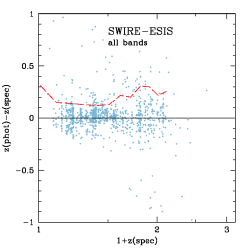
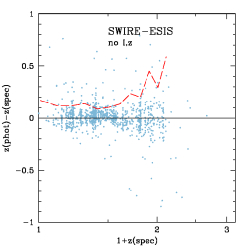
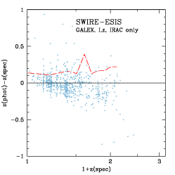
Figure 17: Photometric redshift tests on galaxies in the SWIRE-ESIS field, run with EAZY code (G. Brammer, P. G. van Dokkum & P. Coppi, ApJ submitted). Left: all photometric bands; center: all bands excepted $I$ and $z$; right: GALEX, $I$ and IRAC only. The dashed lines mark the $1\sigma$ scatter in $z_{phot}-z_{spec}$. Spectroscopic data belong to Feruglio et al. (sub.), Sacchi et al. (in prep.) and La Franca et al. (2004).

6.2 Photometric redshift

When dealing with a very large number of sources, as in the case of our wide area survey, the estimate of galaxy redshifts is mainly based on photometric techniques.

Let us check the advantage of introducing VIMOS $I$ and $z$ bands in the estimate of photometric redshifts for the general galaxy population in the SWIRE-ESIS survey, and explore whether the data in hand are sufficient to produce reliable photometric redshifts in those areas not covered by other optical (e.g. BVR) observations.

To this aim, we have exploited the capabilities of the newly public photometric redshift code EAZY (G. Brammer, P. G. van Dokkum & P. Coppi, ApJ submitted), which combines a maximum likelihood (ML) algorithm and Bayesian constraints on the expected redshift distribution of galaxies. Bayesian techniques in photometric redshift estimates have been thoroughly studied and applied to large datasets in the past with good results (e.g. Benítez 2000). An interesting comparison between Bayesian and pure ML techniques was performed by Hildebrandt et al. (2008), who show the advantage of the former, especially in avoiding aliases, minimizing the incidence of interlopers, and providing a reliable estimate of the redshift uncertainties. The EAZY code has the advantage of being very user-friendly and specifically designed for multi-wavelength surveys.

Figure 17 shows the results of these tests, comparing photometric and spectroscopic (Feruglio et al., sub.; Sacchi et al., in prep.; La Franca et al. 2004) redshifts. In the left panel, photometric redshift were estimated by using all the available UV-optical-IR data (GALEX, ESIS, $J,\ K_{s}$, IRAC), while the central panel does not account for $I$ and $z$ data. Finally the right-hand plot shows photometric redshifts obtained including only GALEX, $I$ band and IRAC fluxes (i.e. those data available over the whole ELAIS-S1 area).

When introducing $I$ and $z$ — in combination with all the other available data — one would expect a significant improvement in the photometric redshift estimate. Actually, these data are effective in constraining photometric redshifts, only above redshift $z\sim 0.8$, when the Balmer break lies in or red ward the $R$ band. Unfortunately, only few spectroscopic redshifts are available in this redshift domain, in ELAIS-S1. Nevertheless, one can appreciate some improvement in the scatter of $z_{phot}-z_{spec}$ for $z>0.8$, where $\sigma_{\Delta z}$ reduces from 0.36 to 0.25. No significant improvement is seen at lower redshifts ($\sigma_{\Delta z}\sim 0.15$).

On the other hand, when considering only GALEX, $I$ band and IRAC data, the result reverses. At low redshift the match between photometric and spectroscopic $z$ is reasonably good, and the scatter is not dramatically larger than in the previous cases ($\sigma_{\Delta z}\simeq 0.17$). The code tends to systematically underestimate the redshift, but the drift is smaller than $\Delta(z)\simeq 0.05$. At redshifts larger than $z\sim 0.6$, the results become rather poor: the scatter increases, and the systematic shift is no longer negligible. At $z>0.8$ we have a systematic $\Delta z\simeq-0.15$. This effect can probably be explained with the difficulty to detect galaxies at higher redshift with GALEX. An obvious exception is the case of IR-peakers, for which the IRAC detection of 1.6$\mu$m stellar peak constrains the redshift (e.g. Berta et al. 2007a, b; Weedman et al. 2006).

The fraction of catastrophic outliers increases from 5% to 10%, when using only GALEX, $I$ and IRAC bands.

Generally speaking, Rowan-Robinson et al. (2008) showed that at least 5 different photometric bands are needed, in order to obtain a reliable photometric redshift estimate, including 2 IRAC fluxes, and (for example) 3 optical. ELAIS-S1 will benefit of three additional optical bands over the whole field, once the ESIS-WFI data processing will be completed and presented in a forthcoming paper.

7 Summary

In the era of wide-area cosmological surveys, we have presented $I$ and $z$ band wide field imaging of ELAIS-S1, carried out with the VIMOS camera on VLT. These observations are part of the ESO-Spitzer Imaging extragalactic Survey (ESIS) and cover $\sim 4$ deg² in the $I$ band and $\sim 1$ deg² in $z$. The nominal exposure time is 1800s and 3600s in $I$ and $z$ respectively, but the coverage is not uniform, due to the very complex observing pattern.

As a result of accurate data processing, nine independent mosaics for the $I$ band and one single, 1 deg² wide frame in the $z$ band were produced. The final catalogs include more than 300000 $I$ band sources and 50000 $z$ band objects. Equatorial coordinates of VIMOS objects are constrained within $\sim 0.2$ r.m.s. arcsec, when compared to the GSC 2.2 catalog. Relative astrometric accuracy between the nine $I$ band images is as good as $\sim 0.1$ arcsec r.m.s.

Photometric uncertainties were estimated through simulations, and turn out to be $\sim 0.05,\ 0.20$ mag at $I=21.5,\ 23.5$ and slightly larger in the $z$ band. The survey reaches a 90% average completeness at 23.1 and 22.5 (Vega magnitudes) in the $I$ and $z$ band respectively.

The ESIS VIMOS survey provides optical $I$ counterparts for $>60$% (137206/219877) of SWIRE/Spitzer sources in the ELAIS-S1 area.

We have exploited the new $I$ and $z$ band data — in combination to the other multi-wavelength observations available in ELAIS-S1 — to search for high-redshift ($z=1-3$) galaxies. Our selection is based on the detection of the 1.6$\mu$m stellar peak in the IRAC wavelength domain (IR-peakers Berta et al. 2007a). The $I$ band data give a valuable constraint on IR-peakers: requiring $(I-3.6)_{AB}>2$ avoids low-redshift ($z\mathrel{\hbox{\hbox to0.0pt{\hbox{\lower 4.0pt\hbox{$\sim$}}\hss}\hbox{$<$}}}0.6$) interlopers. The availability of VIMOS data over $\sim 4$ deg² allows the selection to be extended over the whole SWIRE-ESIS field. A total of 973 5.8$\mu$m-peak galaxies at $z=2-3$ were found over $\sim 4$ deg² at the SWIRE 5.8$\mu$m 3$\sigma$ depth (25.8 $\mu$Jy).

The $z$ band data were used to perform the $BzK$ (Daddi et al. 2004) selection over $\sim 1$ deg² and verify the consistency of the IR-peakers class. Our high-$z$ objects lie in the locus of $z>1.4$ star forming galaxies. Apparently, no passive IR-peakers are detected at SWIRE-ESIS depth, over the central ESIS 1 deg² field.

At the SWIRE depth, these galaxies have stellar masses $M>10^{11}$ M_⊙ at $z>2$. The identification of a significant number of these rare high-$z$ sources is possible only thanks to the wide area probed by SWIRE-ESIS. This survey is giving a significant contribution — among others — in studying the very massive tail of the stellar mass function at $z>2$, and constraining the physical properties of its constituents (e.g. Berta et al. 2007a; Lonsdale et al. 2006).

Updates on the ESIS project are available on the web page http://www.astro.unipd.it/esis.

Field	OB	R.A.	Dec.	Date	A.M.	Field	OB	R.A.	Dec.	Date	A.M.
number		$[$hh:mm:ss$]$	$[^{\circ}:^{\prime}:{\arcsec}]$	$[$yyyy-mm-dd$]$		number		$[$hh:mm:ss$]$	$[^{\circ}:^{\prime}:{\arcsec}]$	$[$yyyy-mm-dd$]$
Field 1	A	00:32:48.00	-44:24:00.0	2003-07-08	1.509	Field 26	A	00:38:26.10	-43:30:45.0	2003-11-19	1.258
	B	00:32:59.30	-44:21:36.0	2003-11-18	1.063		B	00:38:37.24	-43:28:21.0	2003-11-18	1.066
	C	00:33:10.59	-44:19:12.0	2003-07-27	1.454		C	00:38:48.35	-43:25:57.0	2003-11-16	1.090
Field 2	A	00:34:13.80	-44:24:00.0	2003-07-08	1.434	Field 27	A	00:39:50.63	-43:30:45.0	2003-11-21	1.383
	B	00:34:25.10	-44:21:36.0	2003-11-21	1.239		B	00:40:01.76	-43:28:21.0	2003-07-10	1.092
	C	00:34:36.38	-44:19:12.0	2003-07-27	1.386		C	00:40:12.88	-43:25:57.0	2003-11-16	1.165
Field 3	A	00:35:39.59	-44:24:00.0	2003-07-08	1.366	Field 28	A	00:41:15.15	-43:30:45.0	2004-08-11	1.064
	B	00:35:50.90	-44:21:36.0	2003-11-17	1.270		B	00:41:26.29	-43:28:21.0	2004-08-21	1.177
	C	00:36:02.18	-44:19:12.0	2003-07-27	1.330		C	00:41:37.41	-43:25:57.0	2004-08-21	1.068
Field 4	A	00:37:05.39	-44:24:00.0	2003-07-08	1.314	Field 29	A	00:32:48.00	-43:13:00.0	2003-08-03	1.059
	B	00:37:16.69	-44:21:36.0	2003-11-18	1.085		B	00:32:59.08	-43:10:36.0	2003-12-19	1.286
	C	00:37:27.98	-44:19:12.0	2003-07-27	1.232		C	00:33:10.15	-43:08:12.0	2004-07-17	1.201
Field 5	A	00:38:31.19	-44:24:00.0	2003-07-08	1.268	Field 30	A	00:34:12.11	-43:13:00.0	2003-12-16	1.086
	B	00:38:42.49	-44:21:36.0	2003-07-09	1.268		B	00:34:23.19	-43:10:36.0	2003-12-21	1.219
	C	00:38:53.78	-44:19:12.0	2003-11-16	1.384		C	00:34:34.26	-43:08:12.0	2004-07-19	1.104
Field 6	A	00:39:56.99	-44:24:00.0	2003-07-08	1.225	Field 31	A	00:35:36.23	-43:13:00.0	2003-12-16	1.389
	B	00:40:08.29	-44:21:36.0	2003-11-18	1.065		B	00:35:47.31	-43:10:36.0	2004-08-21	1.364
	C	00:40:19.57	-44:19:12.0	2003-07-31	1.069		C	00:35:58.37	-43:08:12.0	2004-08-13	1.389
Field 7	A	00:41:22.78	-44:24:00.0	2004-07-12	1.207	Field 32	A	00:37:00.34	-43:13:00.0	2003-12-18	1.175
	B	00:41:34.09	-44:21:36.0	2004-07-14	1.074		B	00:37:11.42	-43:10:36.0	2004-07-22	1.109
	C	00:41:45.37	-44:19:12.0	2004-08-21	1.063		C	00:37:22.49	-43:08:12.0	2004-07-22	1.067
Field 8	A	00:32:48.00	-44:06:15.0	2003-07-08	1.170	Field 33	A	00:38:24.46	-43:13:00.0	2003-07-08	1.060
	B	00:32:59.24	-44:03:51.0	2003-11-18	1.064		B	00:38:35.54	-43:10:36.0	2003-07-10	1.075
	C	00:33:10.47	-44:01:27.0	2003-07-27	1.542		C	00:38:46.60	-43:08:12.0	2003-11-16	1.242
Field 9	A	00:34:13.37	-44:06:15.0	2003-07-08	1.143	Field 34	A	00:39:48.57	-43:13:00.0	2003-11-21	1.461
	B	00:34:24.61	-44:03:51.0	2003-07-09	1.144		B	00:39:59.65	-43:10:36.0	2003-07-10	1.065
	C	00:34:35.84	-44:01:27.0	2003-07-27	1.271		C	00:40:10.72	-43:08:12.0	2003-11-16	1.133
Field 10	A	00:35:38.73	-44:06:15.0	2003-07-08	1.121	Field 35	A	00:41:12.69	-43:13:00.0	2004-08-11	1.073
	B	00:35:49.98	-44:03:51.0	2003-07-09	1.116		B	00:41:23.77	-43:10:36.0	2004-08-20	1.196
	C	00:36:01.21	-44:01:27.0	2003-07-27	1.188		C	00:41:34.83	-43:08:12.0	2004-08-21	1.144
Field 11	A	00:37:04.10	-44:06:15.0	2003-07-08	1.101	Field 36	A	00:32:48.00	-42:55:15.0	2003-08-01	1.112
	B	00:37:15.35	-44:03:51.0	2003-11-18	1.099		B	00:32:59.03	-42:52:51.0	2003-08-03	1.086
	C	00:37:26.57	-44:01:27.0	2003-07-27	1.157		C	00:33:10.04	-42:50:27.0	2003-11-18	1.117
Field 12	A	00:38:29.47	-44:06:15.0	2003-07-08	1.086	Field 37	A	00:34:11.71	-42:55:15.0	2003-11-19	1.054
	B	00:38:40.71	-44:03:51.0	2003-07-09	1.085		B	00:34:22.74	-42:52:51.0	2003-11-18	1.064
	C	00:38:51.94	-44:01:27.0	2003-11-16	1.293		C	00:34:33.75	-42:50:27.0	2003-11-18	1.139
Field 13	A	00:39:54.83	-44:06:15.0	2003-07-08	1.074	Field 38	A	00:35:35.42	-42:55:15.0	2003-11-19	1.054
	B	00:40:06.08	-44:03:51.0	2003-11-18	1.060		B	00:35:46.45	-42:52:51.0	2003-11-19	1.067
	C	00:40:17.31	-44:01:27.0	2003-11-16	1.069		C	00:35:57.46	-42:50:27.0	2003-11-19	1.058
Field 14	A	00:41:20.20	-44:06:15.0	2004-08-18	1.133	Field 39	A	00:36:59.13	-42:55:15.0	2003-11-19	1.076
	B	00:41:31.45	-44:03:51.0	2004-07-14	1.065		B	00:37:09.70	-42:52:51.0	2003-11-16	1.053
	C	00:41:42.68	-44:01:27.0	2004-08-21	1.061		C	00:37:21.17	-42:50:27.0	2003-11-19	1.081
Field 15	A	00:32:48.00	-43:48:30.0	2003-12-17	1.201	Field 40	A	00:38:22.84	-42:55:15.0	2003-11-19	1.205
	B	00:32:59.19	-43:46:06.0	2003-12-21	1.138		B	00:38:33.86	-42:52:51.0	2003-11-16	1.452
	C	00:33:10.36	-43:43:42.0	2004-07-18	1.110		C	00:38:44.88	-42:50:27.0	2003-11-16	1.534
Field 16	A	00:34:12.94	-43:48:30.0	2003-12-16	1.251	Field 41	A	00:39:46.55	-42:55:15.0	2003-11-19	1.369
	B	00:34:24.13	-43:46:06.0	2004-07-25	1.058		B	00:39:57.57	-42:52:51.0	2003-11-18	1.080
	C	00:34:35.31	-43:43:42.0	2004-07-19	1.059		C	00:40:08.59	-42:50:27.0	2003-11-16	1.104
Field 17	A	00:35:37.89	-43:48:30.0	2003-12-17	1.313	Field 42	A	00:41:10.26	-42:55:15.0	2004-07-12	1.163
	B	00:35:49.07	-43:46:06.0	2004-09-06	1.064		B	00:41:21.28	-42:52:51.0	2004-08-20	1.161
	C	00:36:00.25	-43:43:42.0	2004-09-06	1.060		C	00:41:32.29	-42:50:27.0	2004-08-12	1.148
Field 18	A	00:37:02.83	-43:48:30.0	2004-09-06	1.109	Field 43	A	00:32:48.00	-44:41:45.0	2004-06-21	1.152
	B	00:37:14.02	-43:46:06.0	2004-08-15	1.164		B	00:32:59.36	-44:39:21.0	2004-06-23	1.127
	C	00:37:25.19	-43:43:42.0	2004-08-21	1.073		C	00:33:10.70	-44:36:57.0	2004-06-23	1.106
Field 19	A	00:38:27.77	-43:48:30.0	2003-11-19	1.312	Field 44	A	00:34:14.23	-44:41:45.0	2004-06-21	1.127
	B	00:38:38.96	-43:46:06.0	2003-07-09	1.063		B	00:34:25.59	-44:39:21.0	2004-06-26	1.351
	C	00:38:50.14	-43:43:42.0	2003-11-16	1.077		C	00:34:36.94	-44:36:57.0	2004-06-26	1.290
Field 20	A	00:39:52.72	-43:48:30.0	2003-11-21	1.324	Field 45	A	00:35:40.47	-44:41:45.0	2004-06-21	1.095
	B	00:40:03.90	-43:46:06.0	2003-07-10	1.140		B	00:35:51.83	-44:39:21.0	2004-06-26	1.134
	C	00:40:15.08	-43:43:42.0	2003-11-16	1.200		C	00:36:03.17	-44:36:57.0	2004-07-25	1.082
Field 21	A	00:41:17.66	-43:48:30.0	2004-08-20	1.137	Field 46	A	00:37:06.70	-44:41:45.0	2004-06-27	1.123
	B	00:41:28.85	-43:46:06.0	2004-07-24	1.069		B	00:37:18.06	-44:39:21.0	2004-08-15	1.207
	C	00:41:40.02	-43:43:42.0	2004-08-21	1.063		C	00:37:29.41	-44:36:57.0	2004-08-12	1.098
Field 22	A	00:32:48.00	-43:30:40.0	2003-12-17	1.121	Field 47	A	00:38:32.94	-44:41:45.0	2004-06-27	1.104
	B	00:32:59.13	-43:28:21.0	2003-12-19	1.457		B	00:38:44.30	-44:39:21.0	2004-08-12	1.114
	C	00:33:10.25	-43:25:57.0	2004-07-17	1.117		C	00:38:55.64	-44:36:57.0	2004-08-20	1.097
Field 23	A	00:34:12.53	-43:30:45.0	2003-12-16	1.147	Field 48	A	00:39:59.17	-44:41:45.0	2004-06-27	1.089
	B	00:34:23.66	-43:28:21.0	2004-07-17	1.061		B	00:40:10.53	-44:39:21.0	2004-08-20	1.115
	C	00:34:34.78	-43:25:57.0	2004-07-19	1.066		C	00:40:21.88	-44:36:57.0	2004-08-12	1.133
Field 24	A	00:35:37.05	-43:30:45.0	2003-12-18	1.110	Field 49	A	00:41:25.41	-44:41:45.0	2004-08-21	1.226
	B	00:35:48.19	-43:28:21.0	2004-08-21	1.142		B	00:41:36.77	-44:39:21.0	2004-08-21	1.128
	C	00:35:59.30	-43:25:57.0	2004-08-13	1.240		C	00:41:48.11	-44:36:57.0	2004-08-21	1.069
Field 25	A	00:37:01.58	-43:30:45.0	2003-12-18	1.287
	B	00:37:12.71	-43:28:21.0	2004-07-22	1.057
	C	00:37:23.83	-43:25:57.0	2004-08-13	1.066

Table 4: Log file of $I$ band ESIS VIMOS observations.

Field	OB	R.A.	Dec.	Date	A.M.
number		$[$hh:mm:ss$]$	$[^{\circ}:^{\prime}:{\arcsec}]$	$[$yyyy-mm-dd$]$
Field 15	A	00:32:48.00	-43:48:30.0	2003-12-17	1.250
	B	00:32:59.19	-43:46:06.0	2003-12-21	1.174
	C	00:33:10.36	-43:43:42.0	2004-07-18	1.088
Field 16	A	00:34:12.94	-43:48:30.0	2003-12-16	1.311
	B	00:34:24.13	-43:46:06.0	2004-07-25	1.063
	C	00:34:35.31	-43:43:42.0	2004-07-19	1.064
Field 17	A	00:35:37.89	-43:48:30.0	2003-12-17	1.386
	B	00:35:49.07	-43:46:06.0	2004-09-06	1.076
	C	00:36:00.25	-43:43:42.0	2004-09-06	1.058
Field 18	A	00:37:02.83	-43:48:30.0	2004-09-06	1.088
	B	00:37:14.02	-43:46:06.0	2004-08-15	1.130
	C	00:37:25.29	-43:43:46.8	2004-08-21	1.098
Field 22	A	00:32:48.00	-43:30:45.0	2003-12-17	1.154
	B	00:32:59.13	-43:28:21.0	2003-12-19	1.561
	C	00:33:10.25	-43:25:57.0	2004-07-17	1.093
Field 23	A	00:34:12.53	-43:30:45.0	2003-12-16	1.186
	B	00:34:23.66	-43:28:21.0	2004-07-17	1.057
	C	00:34:34.78	-43:25:57.0	2004-07-19	1.058
Field 24	A	00:35:37.05	-43:30:45.0	2003-12-18	1.138
	B	00:35:48.19	-43:28:21.0	2004-08-21	1.181
	C	00:35:59.30	-43:25:57.0	2004-08-13	1.191
Field 25	A	00:37:01.58	-43:30:45.0	2003-12-18	1.372
	B	00:37:12.71	-43:28:21.0	2004-07-22	1.061
	C	00:37:23.83	-43:25:57.0	2004-08-13	1.059
Field 29	A	00:32:48.00	-43:13:00.0	2003-08-03	1.055
	B	00:32:59.08	-43:10:36.0	2003-12-19	1.355
	C	00:33:10.15	-43:08:12.0	2004-07-17	1.159
Field 30	A	00:34:12.11	-43:13:00.0	2003-12-16	1.107
	B	00:34:23.19	-43:10:36.0	2003-12-21	1.273
	C	00:34:34.26	-43:08:12.0	2004-07-19	1.082
Field 31	A	00:35:36.23	-43:13:00.0	2003-12-16	1.478
	B	00:35:47.31	-43:10:36.0	2004-08-21	1.293
	C	00:35:58.37	-43:08:12.0	2004-08-13	1.314
Field 32	A	00:37:00.34	-43:13:00.0	2003-12-18	1.219
	B	00:37:11.42	-43:10:36.0	2004-07-22	1.086
	C	00:37:22.49	-43:08:12.0	2004-07-22	1.058

Table 5: Log file of $z$ band ESIS VIMOS observations.

Appendix A Treatment of fringing in VIMOS $I$ and $z$ band frames

As mentioned in Section 3, the VIMOS $I$ and $z$ band frames suffer a strong fringing that needs to be corrected before photometric calibration and mosaicking. Here we describe the main causes of fringing and the procedure adopted to clean ESIS VIMOS images.

A.1 Fringing effects

At wavelengths shorter than $\sim$7000Å, the silicon layer of VIMOS CCDs absorbs photons efficiently, close to the surface of the chip. On the other hand, in the $I$ and $z$ bands the coefficient of absorption of silicon falls rapidly with increasing wavelength. Consequently a significant number of low energy photons passes through the silicon, which acts as a thin film against the higher index of refraction of the substrate: light is reflected back and forth between the two silicon boundaries (e.g. Malumuth et al. 2003).

The crossing and re-crossing waves mutually interfere, reinforce or cancel in amplitude, depending on their wavelength relative to the film thickness. If the thickness of the Si layer varies across the chip, then “fringes” are formed, following paths of constant thickness.

If the CCD is illuminated by mono-chromatic light, with a proper wavelength, sharp fringes are produced. If a uniform broad-band source is used, the range of wavelengths washes out the appearance of fringes, and their pattern will have a reduced amplitude.

The night sky is dominated by emission lines, particularly at the red end of the optical domain. The fringe pattern formed on VIMOS images in the $I$ and $z$ bands is hence dominated by the combination of the thin-film interference for the different monochromatic sky lines.

The observed fringe patterns therefore depend not only on the silicon thickness across the chip, but also on which lines are strong in the night sky.

Since the composition and conditions of the sky should not vary by large amounts across one night, at a first look the observed fringe patterns do not vary strongly from one image to another. Nevertheless, the amplitude of the fringes, and their strength relative to the uniform sky background may vary significantly. Any continuum variation independent on the line emission does change the uniform background relative to the fringe pattern. Some examples are excess scattered light from the moon or from the sun near twilight.

In addition to changes in the continuum background, also the line strengths may vary, as a consequence of changes in the high-altitude atmospheric conditions (e.g. temperature, solar-wind particles). In this case, if the line ratios change significantly, not only the amplitude of fringes changes, but the whole fringe pattern may shift. Even if the fringe pattern is mostly stable, second-order changes make it very difficult to apply a single pattern to all images taken during a full observing night (see also the description of fringing by Elixir, Magnier & Cuillandre 2004).

A.2 De-fringing

The additive fringing component described in Section A.1 must be removed from all science images, by subtracting a template fringe frame, adequately scaled to the amplitude of fringes in each image.

As the light from stars and galaxies is mainly dominated by continuum emission, with a negligible fraction from emission lines, their contribution to fringing is minimal (see Sect. A.1), and fringes are basically produced by the night sky background.

The ideal fringe pattern frame would be obtained from blank sky images taken in the same conditions as science frames. The optimal estimation of the fringe pattern is thus obtained from the science images themselves: by combining all frames obtained at different pointings across each observing night, it is possible to obtain an improved sky flat field (see Berta et al. 2006) containing the fringe information. The procedure adopted to extract the fringe pattern is as follows:

• first of all, mask all astronomical objects from the science images, by using the objmasks task in the MSCRED IRAF package.

• very bright stars and extended galaxies produce extended halos on the images, which need to be masked manually.

• all science frames are combined together, using object-masks. The result is an improved sky flat field, without any astronomical source, showing strong fringes.

• the fringe pattern is then isolated by dividing the improved sky flat field by a boxcar-median frame.

The fringe pattern frame is finally subtracted from each science image, using an appropriate scaling factor in order to account for the possible changes in fringes intensity, relative to the background, and minimize the residuals.

If sky conditions were perfectly stable across the whole observing night, one could use the same fringe pattern to correct all images taken during the night. In practice — with the exception of few fortunate nights — sky conditions are far from being perfectly consistent for the whole duration of observations and it is necessary to produce several (three or more) fringe frames per night, splitting it in contiguous shorter bits. As a consequence, the number of frames used to produce each pattern decreases.

In the worst cases, it is possible that the frames used to produce a given fringe pattern are not pointing in significantly different regions of the sky. This case is particularly critical if very bright stars lie in the field of view, because there exist regions of the chip where fringes are not sampled, as a consequence of heavy masking of big haloes.

An example of the de-fringing procedure is depicted in Fig. 4, where we show one VIMOS frame before (left panel) and after (right panel) subtracting the fringe pattern (central panel).

After fringe removal, it is finally possible to apply a super-sky-flat (ss-flat) (see Berta et al. 2006) in order to correct for residual second order inhomogeneities in the background. Super-sky-flat frames were produced by combining all de-fringed science frames and masking astronomical sources. Again, because of sky variability, several ss-flat frames were needed during each night.