Underdamped Quantum Ratchets

Abstract

We investigate the quantum ratchet effect under the influence of weak dissipation which we treat within a Floquet-Markov master equation approach. A ratchet current emerges when all relevant symmetries are violated. Using time-reversal symmetric driving we predict a purely dissipation-induced quantum ratchet current. This directed quantum transport results from bath-induced superpositions of non-transporting Floquet states.

An intriguing phenomenon in non-equilibrium transport is the ratchet effect [1, 2, 3], i.e., the emergence of directed motion in the absence of any net bias. Net transport results from an interplay between ac driving, spatio-temporal asymmetries, and non-linearities in a periodic potential. This mechanism provides the basis for an increasing number of experiments ranging from particle transport in biological systems [4] and nano-engines [5] to charge transport in semiconductor heterostructures [6, 7], superconductors [8] and spin transport [9]. Symmetry investigations revealed the necessary conditions on the ac force and the static potential, such that a ratchet current can emerge [10, 12, 11, 13].

A widely employed model for studying the ratchet effect is a one-dimensional periodic potential in which classical Brownian particles move [1, 2, 4, 3, 5]. It describes also the motion of a thermal cloud of cold atoms in an ac-driven optical potential [13]. As the atom cloud is cooled down further, one expects quantum effects to become relevant [14]. The Hamiltonian limit of such quantum ratchets has been studied recently [15, 16, 17]. A more realistic description of quantum ratchets necessitates inclusion of the ubiquitous decoherence and quantum dissipation [18, 19, 20, 21]. For moderate-to-strong dissipation, incoherent tunneling transitions prevail and the quantum ratchet current can be studied within quantum rate theory [18, 19, 20, 21], while in the high-temperature limit, one can employ a Fokker-Planck equation with quantum corrections [22]. For very strong friction, a description in terms of an effective Smoluchowski equation comprising leading-order quantum corrections is appropriate [23]. By contrast, the crossover towards the coherent quantum regime, i.e., the underdamped regime [24], in which already weak decoherence significantly alters the Hamiltonian dynamics, still represents an ambitious challenge.

In this letter we study ac-driven quantum ratchet transport in the technically demanding regime of weak quantum dissipation where quantum coherence and relaxation affect each other. We analyze within a Floquet-Markov description [25] the dynamics on quantum attractors by expanding them into the Floquet states of the corresponding coherent time-dependent system. Then a most intriguing question is whether violation of time-reversal symmetry due to weak quantum dissipation is perceivable in the quantum attractor and in the quantum ratchet current.

1 Model and quantum master equation

A quantum particle in a time-dependent periodic potential obeys the Schrödinger equation

$$\mathrm{i}\hbar\frac{\partial}{\partial t}{\psi}(x,t) = \Big{[}-\frac{\hbar^{2}}{2m}\frac{\partial^{2}}{\partial x^{2}}+V(x,t)\Big{]}\psi(x,t),$$ (1)

$$V(x,t) = V_{0}u(x)-xE(t),$$

where $u(x)=u(x+L)$ with $\mathop{\mathrm{max}}|u(x)|\sim 1$ describes the shape of the $L$-periodic potential. The driving $E(t)$ is a time-periodic field with zero mean, $E(t+\mathcal{T})=E(t)$, $\langle E(t)\rangle_{\mathcal{T}}=0$. Henceforth, we use $1/k_{L}\equiv L/2\pi$, $(m/k_{L}^{2}V_{0})^{1/2}$, and $V_{0}$ as units of distance, time, and energy, respectively, such that formally $k_{L}=m=V_{0}=1$, while $\hbar$ becomes the effective Planck constant $\hbar k_{L}/\sqrt{mV_{0}}$ [14].

By the gauge transformation $|\psi\rangle\rightarrow\exp(-\frac{\mathrm{i}}{\hbar}xA(t))|\psi\rangle$, we bring the Schrödinger equation (1) to the spatially periodic form [17]

$$\mathrm{i}\hbar\frac{\partial}{\partial t}{\psi}(x,t)=\Big{(}\frac{1}{2}[\hat{p}-A(t)]^{2}+u(x)\Big{)}\psi(x,t),$$ (2)

with the vector potential $A(t)=-\int_{0}^{t}E(t^{\prime})dt^{\prime}$ and the momentum operator $\hat{p}=-\mathrm{i}\hbar\partial/\partial x$. The corresponding Hamiltonian has recently been realized in cold atom experiments [14]. The Schrödinger equation (2) is time periodic with period $\mathcal{T}=2\pi/\omega$ and, thus, according to the Floquet theorem, it possesses a complete set of mutually orthogonal solutions of the form $|\psi_{\alpha}(t)\rangle=\mathrm{e}^{-\mathrm{i}{\epsilon_{\alpha}}t/{\hbar}}|\phi_{\alpha}(t)\rangle$. The Floquet states $|\phi_{\alpha}(t)\rangle=|\phi_{\alpha}(t+\mathcal{T})\rangle$ and the quasienergies $\epsilon_{\alpha}$, $-\hbar\omega/2<\epsilon_{\alpha}<\hbar\omega/2$, are obtained from the eigenvalue problem $[H(t)-\mathrm{i}\hbar\partial/\partial t]|\phi(t)\rangle=\epsilon|\phi(t)\rangle$ [26]. Owing to discrete translation invariance, all Floquet states are characterized by a quasi momentum $\kappa$ with $|\phi_{\alpha}(x+2\pi)\rangle=\exp(\mathrm{i}\hbar\kappa)|\phi_{\alpha}(x)\rangle$. We restricted our study to states with $\kappa=0$, which can be expanded into the plane waves $|n\rangle=(2\pi)^{-1/2}\exp(\mathrm{i}nx)$. Physically, these states correspond to initial states with atoms populating all wells of the spatial potential equally. Such initial conditions are the natural ones for the recently proposed [27] ring-shaped optical potentials which have already been realized experimentally [28].

We incorporate decoherence and dissipation by coupling the driven system (2) to a bath of non-interacting harmonic oscillators [29]. Following a standard approach to weak quantum dissipation [25], we decompose the reduced density operator $\varrho$ into the Floquet basis of the coherent system, $\varrho_{\alpha\beta}(t)=\langle\phi_{\alpha}(t)|\varrho(t)|\phi_{\beta}(t)\rangle$. Assuming that dissipative effects are relevant only on time scales much larger than the driving period $\mathcal{T}$, we arrive at the master equation

$$\dot{\varrho}_{\alpha\beta}=-\frac{\mathrm{i}}{\hbar}(\epsilon_{\alpha}-\epsilon_{\beta})\varrho_{\alpha\beta}+\sum_{\alpha^{\prime}\beta^{\prime}}\mathcal{L}_{\alpha\beta,\alpha^{\prime}\beta^{\prime}}\,\varrho_{\alpha^{\prime}\beta^{\prime}},$$ (3)

with the time-independent transition rates

$$\begin{split}\mathcal{L}_{\alpha\beta,\alpha^{\prime}\beta^{\prime}}=&\sum_{n}(N_{\alpha\alpha^{\prime},n}+N_{\beta\beta^{\prime},n})X_{\alpha\alpha^{\prime},n}X_{\beta\beta^{\prime},-n}\\ &-\delta_{\beta\beta^{\prime}}\sum_{\beta^{\prime\prime},n}N_{\beta^{\prime\prime}\alpha^{\prime},n}X_{\alpha\beta^{\prime\prime},-n}X_{\beta^{\prime\prime}\alpha^{\prime},n}\\ &-\delta_{\alpha\alpha^{\prime}}\sum_{\alpha^{\prime\prime},n}N_{\alpha^{\prime\prime}\beta^{\prime},n}X_{\beta^{\prime}\alpha^{\prime\prime},-n}X_{\alpha^{\prime\prime}\beta,n}\,,\end{split}$$ (4)

where $X_{\alpha\beta,n}=\langle\langle\phi_{\alpha}(t)|x\,\mathrm{e}^{-\mathrm{i}n\omega t}|\phi_{\beta}(t)\rangle\rangle_{\mathcal{T}}$ and $N_{\alpha\beta,n}=N(\epsilon_{\alpha}-\epsilon_{\beta}+n\hbar\omega)$ with $N(\epsilon)=({\gamma\epsilon}/{\hbar^{2}})n_{\rm th}(\epsilon)$. Here $n_{\rm th}(\epsilon)=[\exp({\epsilon/k_{\rm B}T})-1]^{-1}$ is the thermal occupation number and $\langle\cdots\rangle_{\mathcal{T}}$ denotes the average over one driving period.

This Markov approximation requires that the coupling strength $\gamma$ is the smallest frequency scale in the problem, such that $\gamma\ll k_{\rm B}T/\hbar$ and $\gamma\ll\Delta_{\alpha\beta}/\hbar$, where $\Delta_{\alpha\beta}=|\epsilon_{\alpha}-\epsilon_{\beta}|$ is any splitting of the Floquet spectrum [25]. The latter condition is rather strict because in the present case, the quasienergies are even dense on the interval $[-\hbar\omega/2,\hbar\omega/2]$. Thus, the condition $\gamma\ll\Delta_{\alpha\beta}/\hbar$ is violated for any finite dissipation strength. Yet it is obvious that only a finite number of Floquet states significantly contributes to the density matrix at large times. We thus validate our results for the asymptotic state $\varrho_{\alpha\beta}$ with the following criterion: We sort the Floquet states according to their weights $\varrho_{\alpha\alpha}$ and consider only results for which the first $N_{\varepsilon}$ states fulfill the condition $\gamma/\Delta_{\alpha\beta}<\varepsilon$, where $\varepsilon$ is the threshold value.

For any initial density operator $\varrho_{\alpha\beta}(0)$, the solution of the master equation (3) converges to a unique “quantum attractor” being the fixed point $\varrho_{\alpha\beta}^{a}=\varrho_{\alpha\beta}(t\rightarrow\infty)$ of the quantum master equation. Note that in the Schrödinger picture, the density operator is periodically time-dependent and, thus, describes a limit cycle. Since in Floquet representation, the attractor $\varrho^{a}_{\alpha\beta}$ is nevertheless time-independent, the asymptotic current, defined as the time-averaged momentum expectation value, reads

$$J=\sum_{\alpha\beta}\varrho^{a}_{\alpha\beta}\bar{p}_{\alpha\beta};\quad\bar{p}_{\alpha\beta}=\langle\langle\phi_{\alpha}(t)|\hat{p}|\phi_{\beta}(t)\rangle\rangle_{\mathcal{T}}.$$ (5)

A frequently used simplification is possible if dissipative effects are relevant only on time scales longer than any $2\pi\hbar/(\epsilon_{\alpha}-\epsilon_{\beta}-\epsilon_{\alpha^{\prime}}+\epsilon_{\beta^{\prime}})$. Then, one can employ a full rotating-wave approximation (RWA) for which the diagonal and off-diagonal density matrix elements decouple, such that the quantum attractor becomes diagonal, i.e., $\varrho^{a}_{\alpha\beta}=\varrho^{a}_{\alpha\alpha}\delta_{\alpha\beta}$.

2 Symmetries

Before evaluating the ratchet current we determine two symmetry conditions under which the current vanishes. The first one is the generalized parity $S:(x,t)\to(-x,t+\mathcal{T}/2)$ [26], which is present if the potential and the driving field fulfill the relations

$$u(-x)=u(x);\quad E(t+\mathcal{T}/2)=-E(t).$$ (6)

Then, the Floquet states obey $\phi_{\alpha}(-x,t+\mathcal{T}/2)=\sigma_{\alpha}\phi_{\alpha}(x,t)$, where $\sigma_{\alpha}=\pm 1$ according to the generalized parity. As a consequence, we find $\bar{p}_{\alpha\beta}=-\sigma_{\alpha}\sigma_{\beta}\bar{p}_{\alpha\beta}$ and thus in particular $\bar{p}_{\alpha\alpha}=0$. This means that all Floquet states are non-transporting on time-average [17], such that any non-vanishing current must stem from off-diagonal density matrix elements. The master equation (3) inherits a symmetry from the position matrix elements for which the relation $X_{\alpha\beta n}=(-1)^{n+1}\sigma_{\alpha}\sigma_{\beta}X_{\alpha\beta n}$ holds [12]. This leads to the conclusion that the asymptotic state obeys $\varrho^{a}_{\alpha\beta}=\sigma_{\alpha}\sigma_{\beta}\varrho^{a}_{\alpha\beta}$. Inserting these symmetry relations into expression (5) yields $J=-J$, which implies that the ratchet current vanishes in the presence of generalized parity.

A second relevant symmetry is time-reversal symmetry $t\to-t$. It has the consequence that if $\varrho(t)$ is a solution of the master equation (3), then $\varrho(-t)$ is a solution as well. Time-reversal symmetry is present if the driving field obeys

$$E(t+t_{\mathrm{s}})=E(-t+t_{\mathrm{s}}),$$ (7)

with some appropriate time shift $t_{\mathrm{s}}$, and obviously can persist only in the Hamiltonian limit $\gamma=0$, for which the dynamics depends on the initial conditions. In the Hamiltonian limit, a meaningful ratchet current requires averaging over all possible initial conditions.

Let us again emphasize that all in the presence of either of the two symmetries in eqs. (6), (7), Floquet states are non-transporting such that their current $\bar{p}_{\alpha\alpha}$ vanishes, cf. Ref. [17]. Since within full RWA by construction $\varrho^{a}_{\alpha\beta}=0$ for $\alpha\neq\beta$, while $\bar{p}_{\alpha\alpha}=0$, the current (5) vanishes within this approximation as well. This in turn means that the purely dissipation-induced ratchet current studied below can be obtained only from the full master equation (3).

In order to observe a quantum ratchet current, we need to specify the periodic potential $u(x)$ and the driving field $E(t)$ such that at least one of the conditions in eq. (6) is violated. One possibility would be to use a non-reflection-symmetric static potential $u(x)$ together with a sinusoidal driving [30]. Here, by contrast, we consider a symmetric potential and a bichromatic driving field, i.e.,

$$u(x)=\cos(x);\quad E(t)=E_{1}\cos(\omega t)+E_{2}\cos(2\omega t+\theta),$$ (8)

which breaks generalized parity provided that both $E_{1}$ and $E_{2}$ are non-zero [17]. Indeed, if either $E_{1}=0$ or $E_{2}=0$, the ratchet current vanishes, both classically and quantum mechanically. The phase lag $\theta$ allows one to control the time-reversal symmetry: If $\theta$ is a multiple of $\pi$, the driving field obeys the symmetry condition (7). For any other phase lag and $E_{1},E_{2}\neq 0$, time-reversal symmetry is broken, as can be seen in the Husimi functions [31] of the Floquet states depicted in fig. 1. Moreover, since the transformation $(x,\theta)\rightarrow(-x,\theta\pm\pi)$ leaves the Hamiltonian (2) invariant while it inverts the current, we find that in the Hamiltonian limit, the ratchet current obeys [17]

$$J(\theta)=-J(\theta+\pi)=-J(-\theta).$$ (9)

Notably, this relation does not hold for finite dissipation strength $\gamma>0$.

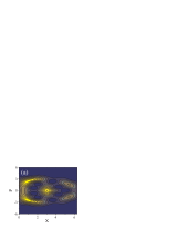
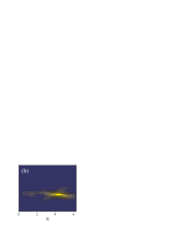
Figure 1: (Color online) Husimi representation of the eigenstate for the potential (8) for phase lag $\theta=0$ (a) and $\theta=-\pi/2$ (b). The corresponding momenta are $\bar{p}_{\alpha\alpha}=0$ (a) and $\bar{p}_{\alpha\alpha}\approx-0.15$ (b) (in units of the recoil momentum). The eigenstate has been tracked along the corresponding quasienergy band. The parameters are $\hbar=0.5$, $E_{1}=1.6$, $E_{2}=2$, $\omega=1$.

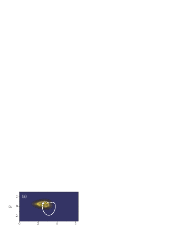
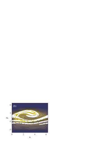
Figure 2: (Color online) Husimi representation of the quantum attractor at stroboscopic times with the corresponding classical attractor superimposed (white dots) for $E_{1}=E_{2}=2$, $\gamma=0.1$, $k_{\mathrm{B}}T=0.1$. Driving frequency, phase lag, and effective Planck constant are $\omega=2$, $\theta=\pi/2$, $\hbar=0.1$ (a) and $\omega=0.87$, $\theta=-\pi/2$, $\hbar=0.2$ (b). The white line in panel (a) marks the corresponding limit cycle. The numerical integration has been performed with 45 basis states and $\varepsilon=0.3$.

3 Quantum ratchet current and quantum attractor

We start out our numerical studies of the dissipative quantum system by validating our master equation approach for the quantum-classical correspondence. Already a classical Brownian particle in the driven periodic potential (8) exhibits a rather rich dynamics, ranging from regular limit cycles to chaotic motion on strange attractors, see fig. 2. The corresponding quantum dynamics is even more complex: In the deep quantum regime $\hbar\geq 1$, it is restricted to a few Floquet states. In the semiclassical regime $\hbar\ll 1$, by contrast, many levels play a role and, thus, we expect to find in the Husimi representation of the density operator signatures of the classical phase-space structure. This represents a demanding requirement for our master equation formalism. In order to emphasize the power of the Floquet master equation (3), we plotted the Husimi function of the quantum attractor for both a regular limit cycle [fig. 2(a)] and a strange attractor [fig. 2(b)]. Comparison with the corresponding classical attractors underlines that our formalism is able to cope with the semiclassical limit.

Since the classical attractor shown in fig. 2(a) is bounded, it is non-transporting, $J_{\mathrm{cl}}=0$. The quantum attractor, by contrast, supports a very small, but finite dc current, $J_{\mathrm{qm}}\simeq 0.0025$. Note that the dc current for the chaotic attractor shown in fig. 2(b) is much larger, namely $J_{\mathrm{cl}}=0.45$ and $J_{\mathrm{qm}}=0.32$, respectively.

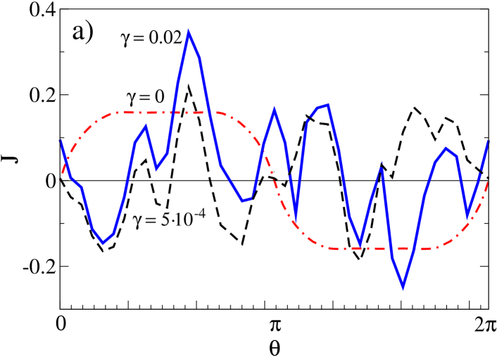
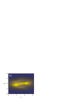
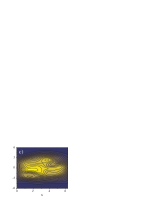
Figure 3: (Color online) (a) Average current $J$ (in units of the recoil momentum) as a function of the phase lag $\theta$ for dissipation strength $\gamma=0.02$ (solid line) and $\gamma=5\times 10^{-4}$ (dashed) compared to the Hamiltonian case (dash-dotted). The inset shows the current for $\theta=0$ as a function of the dissipation strength $\gamma$. Lower panel: Husimi representation of quantum attractors at stroboscopic times $t=nT$ for $\theta=0$: (b) $\gamma=5\cdot 10^{-4}$ and (c) $\gamma=0.02$. The parameters are $\hbar=1$, $E_{1}=1.6$, $E_{2}=2$, $\omega=1$, and $k_{\mathrm{B}}T=0.5$. The numerical integration has been performed with 21 basis states and $\varepsilon=0.3$

Figure 3(a) depicts the ratchet current as a function of the phase lag $\theta$ for different dissipation strengths. In the Hamiltonian limit $\gamma=0$, the current vanishes at the symmetry points $\theta=0,\pi$ as discussed above. Moreover, it complies with relation (9). For finite dissipation, the current exhibits multiple current reversals upon changing the phase lag $\theta$. This feature is already very pronounced for $\gamma=5\cdot 10^{-4}$, which emphasizes that even very weak dissipation changes the behavior significantly. For much stronger dissipation, $\gamma=0.02$, the magnitude of the current changes slightly, while we still observe similar current reversals. For classical dissipative ratchets, such current reversals have been attributed to tangent bifurcations when going from limit cycles towards strange attractors [32]. In the Hamiltonian limit of the quantum dynamics, however, these bifurcations are absent. Therefore, the quantum current reversals may be attributed to dissipation as well.

We next focus on the symmetry point $\theta=0$, where the Hamiltonian system (2) is time-reversal symmetric and non-transporting. Time-reversal symmetry implies invariance under $p\to-p$, which is perceivable in the Husimi representation of the Floquet states at stroboscopic times shown in fig. 1(a). Finite dissipation, however, destroys time-reversal symmetry, such that the attractor looses the symmetry $p\to-p$, see fig. 3(b,c), despite the fact that it is composed of symmetric, non-transporting Floquet states. This reveals that genuine quantum coherence, i.e. off-diagonal density matrix elements, play a crucial role for both the shape of the attractor and the ratchet current. Figure 4(a) shows the dependence of the ratchet current on the dissipation strength $\gamma$. Both for $\gamma=0$ and in the limit $\gamma\to 0$, the current vanishes. For $\gamma>0$ we observe a purely dissipation-induced quantum ratchet current. This current is negative for faint dissipation, but crosses zero and becomes positive with increasing dissipation. This current reversal behavior resembles the one found for the corresponding classical problem [33], but even there has not been explained analytically. The dependence of the ratchet current on the amplitude of the second harmonic, $E_{2}$ in (8), is shown on Fig. 4(b).

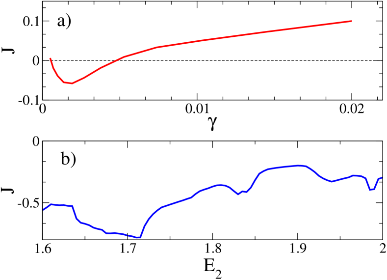
Figure 4: (Color online) (a) Average current $J$ (in units of the recoil momentum) as a function of (a) the dissipation strength $\gamma$ ($E_{2}=2$, $\theta=0$) and (b) as a function of the second harmonic amplitude, $E_{2}$ in (8) ($\gamma=0.02$, $\theta=\pi/2$). The other parameters are the same as in Fig.3.

4 Approaching the Hamiltonian limit

For dissipative chaotic quantum systems, the limit of vanishing dissipation, $\gamma\to 0$, deserves some attention. This will reveal an intriguing difference between classical and quantum ratchets. Already in the presence of arbitrarily small dissipation, the classical phase-space flow converges to a generally unique attractor, while a Hamiltonian system in principle preserves memories to its initial state for an arbitrarily long time. Thus, for $\gamma=0$, the classical current generally depends on the initial conditions, in particular, if the initial phase-space distribution overlaps with regular manifolds [34]. If the initial condition lies within a chaotic manifold, however, the system will in the long-time limit be distributed uniformly over the chaotic manifold and, thus, will eventually become independent of the initial condition [11, 15]. For the corresponding quantum system, this ergodicity is not found owing to the linearity of the Schrödinger equation in combination with the finite number of states involved. As a consequence, the limit of arbitrarily weak dissipation, $\gamma\to 0$, may for quantum systems be different from the Hamiltonian case, $\gamma=0$, as we observe in fig. 3(a).

5 Conclusions

We have studied the quantum ratchet effect in the weakly dissipative regime in which the quantum coherence suffers from decoherence and relaxation. A central property of the corresponding, unique quantum attractor is a quantum ratchet current, given by the time-averaged momentum expectation value. We found that even for very weak dissipation, the current differs strongly from its corresponding Hamiltonian counterpart. The presence of any of two symmetries, namely generalized parity and, in the Hamiltonian limit, time-reversal symmetry, inhibits a ratchet current. For bichromatic driving, the phase lag $\theta$ between the two harmonics determines whether the Hamiltonian part is time-reversal symmetric or not. If time reversal holds, the current vanishes in the Hamiltonian limit, while for finite dissipation, we observe a purely dissipation-induced quantum ratchet current which, moreover, possesses current reversals as a function of the dissipation strength.

For cold atoms, the resulting currents are of the order 10–30% of the recoil momentum, being measurable with present experimental techniques [14]. Our study provides evidence that cold atoms in driven periodic potentials are a natural candidate for studying the complex dynamics originating from an intriguing interplay of nonlinearity, weak quantum dissipation, and spatio-temporal symmetry violation.

- [1] \NameSmoluchowski, M. v. \REVIEWPhys. Zeitschr.1319121069.
- [2] \NameReimann P. Hänggi P. \REVIEWAppl. Physics A752002169; \NameHänggi P. Marchesoni F. \REVIEWRev. Mod. Phys.in pressarXiv:0807.1283
- [3] \NameReimann P. \REVIEWPhys. Rep.361200257.
- [4] \NameJülicher F., Ajdari A. Prost J. \REVIEWRev. Mod. Phys.6912691997.
- [5] \NameAstumian R. D. Hänggi P. \REVIEWPhys. Today55 (11)200233; \NameHänggi P., Marchesoni F. Nori F. \REVIEWAnn. Phys. (Leipzig)14200551.
- [6] \NameLinke H. et al. \REVIEWScience28619992314.
- [7] \NameKhrapai V. S. et al. \REVIEWPhys. Rev. Lett.972006176803.
- [8] \NameMajer J. B. et al. \REVIEWPhys. Rev. Lett.902003056802.
- [9] \NameSmirnov S., Bercioux D., Grifoni M. Richter K. \REVIEWPhys. Rev. Lett.1002008230601.
- [10] \NameFlach S., Yevtushenko O. Zolotaryuk Y. \REVIEWPhys. Rev. Lett.8420002358.
- [11] \NameDenisov S. et al. \REVIEWPhys. Rev. E662002041104.
- [12] \NameLehmann J., Kohler S., Hänggi P. Nitzan A. \REVIEWJ. Chem. Phys.11820033283.
- [13] \NameSchiavoni M., Sanchez-Palencia L., Renzoni F. Grynberg G., \REVIEWPhys. Rev. Lett.902003094101; \NameGommers R., Denisov S. Renzoni F. \REVIEWPhys. Rev. Lett.962006240604.
- [14] \NameMorsch O. Oberthaler M. \REVIEWRev. Mod. Phys.782006179.
- [15] \NameSchanz H., Otto M.-F., Ketzmerick R. Dittrich T. \REVIEWPhys. Rev. Lett.872001070601; \NameSchanz H., Dittrich T. Ketzmerick R. \REVIEWPhys. Rev. E712005026228.
- [16] \NameCarlo G. G. et al. \REVIEWPhys. Rev. A742006033617.
- [17] \NameDenisov S., Morales-Molina L., Flach S. Hänggi P. \REVIEWPhys. Rev. A752007063424.
- [18] \NameReimann P., Grifoni M. Hänggi P. \REVIEWPhys. Rev. Lett.79199710.
- [19] \NameGoychuk I. Hänggi P. \REVIEWEurophys. Lett.431998503; \NameGoychuk I., Grifoni M. Hänggi P. \REVIEWPhys. Rev. Lett.811998649; \SAME8119982837.
- [20] \NameGrifoni M., Ferreira M. S., Peguiron J. Majer J. B. \REVIEWPhys. Rev. Lett.892002146801.
- [21] \NameScheidl S. Vinokur V. M. \REVIEWPhys. Rev. B652002195305.
- [22] \NameZueco D. Garcia-Palacios J. L. \REVIEWPhysica E292005435.
- [23] \NameMachura L. et al. \REVIEWPhys. Rev. E702004031107.
- [24] \NameCarlo G. G., Benenti G., Casati G. Shepelyansky D. L. \REVIEWPhys. Rev. Lett.942005164101.
- [25] \NameKohler S., Dittrich N. Hänggi P. \REVIEWPhys. Rev. E551997300.
- [26] \NameGrifoni M. Hänggi P. \REVIEWPhys. Rep.3041998232.
- [27] \NameAmico L., Osterloh A., Cataliotti F. \REVIEWPhys. Rev. Lett. 952005063201.
- [28] \NameFranke-Arnold S. et al \REVIEWOpt. Exp. 1520078619.
- [29] \NameCaldeira A. O. Leggett A. L. \REVIEWAnn. Phys. (N.Y.)1491983374.
- [30] \NameSalger T., Geckeler C., Kling S. Weitz M. \REVIEWPhys. Rev. Lett.992007190405.
- [31] \NameHusimi K. \REVIEWProc. Phys. Math. Soc. Japan221940264.
- [32] \NameMateos J. \REVIEWPhys. Rev. Lett. 842000258.
- [33] \NameYevtushenko O., Flach S., Zolotaryuk Y. Ovchinnikov A. A. \REVIEWEurophys. Lett. 542001141.
- [34] \NameZaslavsky G. M. \BookPhysics of Chaos in Hamiltonian Systems \PublImperial College Press, London \Year1989.