Top BSM at D0

Abstract

The D0 experiment has searched for phenomena beyond the standard model in top quark events. The methods and results of four analyses covering various possible deviations from the standard model behaviour are discussed. With data sets covering up to $2.1\,\mbox{fb}^{-1}$ no deviation from the standard model expectations could be found.

1 Introduction

Since the top was discovered by CDF and D0 at the Tevatron in 1995 [1, 2] the number of top events available for experimental studies has been increased by more than an order of magnitude. Tevatron now delivered a luminosity of more than $4\,\mbox{fb}^{-1}$ up to half of which has been analysed for top quark analyses in D0. These data are, amongst other studies, investigated to verify whether the events selected as top quarks actually behave as expected by the Standard Model (SM).

The questions one may ask to challenge the SM-likeness of the top quark naturally fall into 4 categories. First, one may ask whether the events that are considered to be top quarks actually are all top quarks or whether some additional unknown new particle is hiding in the selected data. Second one may ask whether the top quark decay looks as predicted by the SM, maybe a contribution from a new particle can be detected. Third one may ask whether the quantum numbers of the top are the expected ones or whether exotic scenarios play a role. And fourth one may ask if non-standard production mechanisms add to the SM diagrams.

The analyses considered address these questions within the selections used to detect one of the SM decay channels of the top quark. For top pair production these are defined by the decay of two $W$ bosons as dilepton, $\ell+$jets and all hadronic channel. This writeup covers one D0 analysis for each of the above questions using data selected in one or more of the top pair decay channels. Additional analyses of top events with interpretations beyond the standard model are discussed elsewhere in these proceedings [3, 4].

2 Search for Stop Admixture

A particle that may hide in the samples usually considered to be top quarks are its supersymmetric partners, the stop quarks, $\tilde{t}_{1}$ and $\tilde{t}_{2}$. The stop decay modes to neutralino and top quark, $\tilde{\chi}_{1}^{0}t$, or through chargino and $b$ quark, $\tilde{\chi}_{1}^{\pm}b$, both yield neutralino, $b$ quark and $W$ boson, $\tilde{\chi}_{1}^{0}bW$. The neutralino is the lightest supersymmetric particle in many models and is stable if $R$-parity in conserved. Then it escapes the detector and the experimental signature of stop pair production differs from that of top pair production only by the additional contribution to the missing transverse energy from the neutralino.

2.1 Data Selection, Signal and Background Description

D0 has searched for a contribution of such stop pair production in the semileptonic channel in data with $\sim\!0.9\,\mbox{fb}^{-1}$[5]. Semileptonic events were selected following the corresponding $t\bar{t}$ cross-section analysis by looking for isolated leptons ($e$ and $\mu$), missing transverse energy and four or more jets. At least one of the jets was required to be identified as $b$-jet using D0’s neural network algorithm. To describe the SM expectation a mixture of data and simulation (MC) is employed. The description of top pair production (and of further minor backgrounds) is taken fully from MC normalised to the corresponding theoretical cross-sections. For $W+$jets the kinematics is taken from MC, but the normalisation is taken from data. Multijet background is fully estimated from data. As signal we consider the lighter of the two stop quarks, $\tilde{t}_{1}$. Production of $\tilde{t}_{1}\bar{\tilde{t}}_{1}$ is simulated for various combinations of stop and chargino masses, $m_{\tilde{t}_{1}},m_{\tilde{\chi}^{\pm}_{1}}$. For the sake of this analysis the stop mass was chosen to be less or equal to the top mass. The neutralino mass $m_{\tilde{\chi}^{0}_{1}}=50\,\mbox{Ge\kern-0.86108ptV}$ was chosen to be close to the experimental limit.

2.2 Signal Background Separation

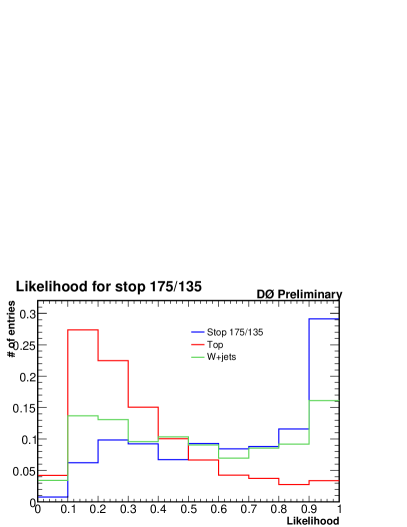
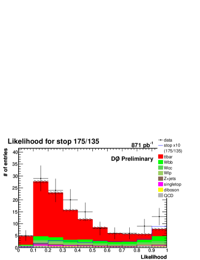
Figure 1: Likelihood distribution $m_{\tilde{t}_{1}}=175\,\mbox{Ge\kern-0.86108ptV}$, $m_{\tilde{\chi}_{1}^{\pm}}=135\,\mbox{Ge\kern-0.86108ptV}$. Left: Expected shape for stop signal, SM top pairs and $W+$jets events. Right: Expected distribution for SM compared to data. The stop contribution expected in the MSSM is enhanced by a factor of 10.

To detect a possible contribution of stop pairs the differences between stop pair events and SM top pair production kinematic variables are combined into a likelihood, ${\cal L}=P_{\mathrm{stop}}/\left(P_{\mathrm{stop}}+P_{\mathrm{SM}}\right)$. The kinematic variables considered include the transverse momentum of the (leading) $b$ jet, distances between leading $b$ jet and lepton or leading other jet. Additional variables were reconstructed by applying a constraint fit. In this fit reconstructed physics objects (lepton, missing transverse energy and jets) are assigned to the decay products of an assumed semileptonic top pair event and the measured quantities are allowed to vary within their experimental resolution to fulfil additional constraints. It was required that the $W$ mass is consistent with the invariant mass of the jets assigned to the two light quarks as well as with the invariant mass of the lepton with the neutrino. The masses of the reconstructed top pairs were constrained to be equal. Of the possible jet parton assignments only the one with the best $\chi^{2}$ was used. From the constraint fits observables the angle between the $b$-quarks and the beam axis in the $b\bar{b}$ rest frame, the $b\bar{b}$ invariant mass, the distances between the $b$’s and the same-side or opposite-side $W$ bosons and the reconstructed top mass are considered. The likelihood was derived for each $m_{\tilde{t}_{1}},m_{\tilde{\chi}^{\pm}_{1}}$ combination separately and the selection of variables used has been optimised each time. Figure 1 shows the separation power of the likelihood for the case of $m_{\tilde{t}_{1}}=175\,\mbox{Ge\kern-0.86108ptV}$, $m_{\tilde{\chi}^{\pm}_{1}}=135\,\mbox{Ge\kern-0.86108ptV}$ and the comparison to the observed data.

2.3 Limits and Cross Checks

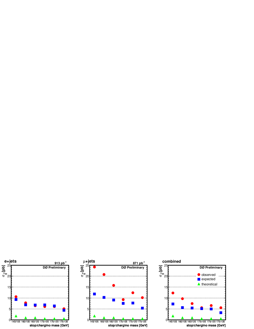
Figure 2: Expected and observed limits on the stop pair production cross-section compared to the expectation in the MSSM for $e+$jets (left), $\mu+$jets (middle) and combined data (right).

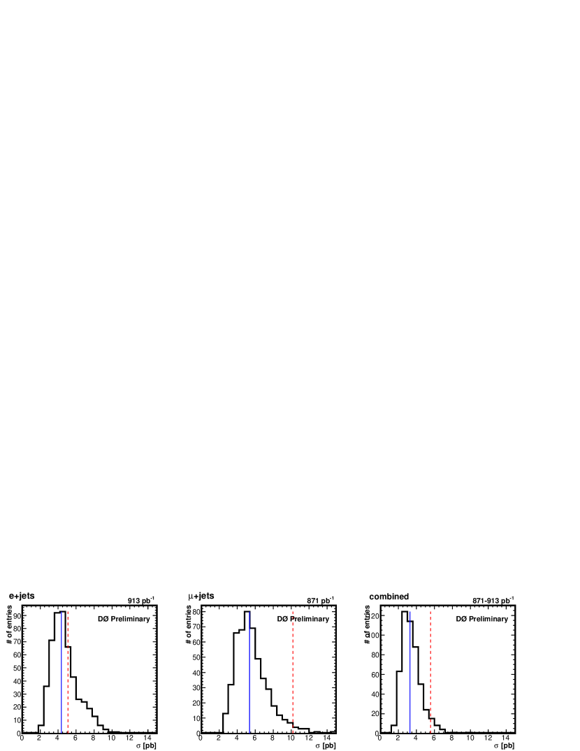
Figure 3: Distribution of results for $m_{\tilde{t}}=175\,\mbox{Ge\kern-0.86108ptV}$, $m_{\tilde{\chi}^{\pm}}=135\,\mbox{Ge\kern-0.86108ptV}$ obtains in 500 sets of SM pseudo data. The expected and observed results are shown as full and dashed lines, respectively.

To determine limits on the possible contribution of stop pair production in the selected channel Bayesian statistics is employed using a non-zero flat prior (for positive values) of the stop pair cross-section. A Poisson distribution is assumed for the number of events observed in each bin of the likelihood. The prior for the combined signal acceptance and background yields is a multivariate Gaussian with uncertainties and correlations described by a covariance matrix. The systematic uncertainty is dominated by the uncertainties on the theoretical cross-section of top pair production, on the selection efficiencies and the luminosity determination. Figure 2 shows the expected and observed limits on the stop pair production cross-section compared to the MSSM prediction for various values of $m_{\tilde{t}_{1}}$ and $m_{\tilde{\chi}^{\pm}_{1}}$. While the $e+$jets channel shows agreement between observed and expected limits, the observed limits in the $\mu+$jets channel are weaker than the expectations. In all cases the theoretically expected stop signal cross-section in the MSSM is much smaller than the experimental limits. Still, the deviation of the observed from the expected limit in the $\mu+$jets data may be a sign of new physics. To estimated the consistency of the observation with the SM, 500 sets of SM pseudo data were generated and the analysis was repeated on each of these pseudo datasets. The distribution of limit results is shown in Fig. 3 for the example of $m_{\tilde{t}_{1}}=175\,\mbox{Ge\kern-0.86108ptV}$, $m_{\tilde{\chi}^{\pm}_{1}}=135\,\mbox{Ge\kern-0.86108ptV}$. The distributions exhibit a strong asymmetry towards higher limits and some percent of the pseudo data yield a limit even higher than the one observed in real data. D0 thus concludes that the observed results are consistent with a statistical fluctuation within the SM.

3 Search for Decay to Charged Higgs

New particles in the final state of top pair events may alter the branching fractions to the various decay channels. Because measured top pair production cross-sections, $\sigma_{t\bar{t}}$, are calculated assuming the SM branching fraction, this would be visible by comparing $\sigma_{t\bar{t}}$ measured in various channels.

In a first analysis D0 considers the case of a charged Higgs replacing the $W$ in the top decay [6]. The charged Higgs is assumed to decay hadronically. Within the MSSM with its two Higgs doublets this case is relevant for low values of $\tan\beta$. General multi-Higgs-doublet models allow such leptophobic charged Higgs’ over a large range of parameters. The observable employed is the cross-section ratio $R_{\sigma}=\sigma_{t\bar{t}}^{\ell+\mathrm{jets}}/\sigma_{t\bar{t}}^{\mathrm{Dilepton}}$.

3.1 Determination of the Cross-Section Ratio

The determination of cross-section ratio, $R_{\sigma}$, is based on individual cross-section measurements in the $\ell+$jets and the dilepton channel, that are based on luminosity of $\sim\!0.9\,\mbox{fb}^{-1}$ and $\sim\!1.0\,\mbox{fb}^{-1}$, respectively.

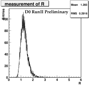
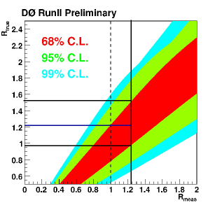
Figure 4: Left: Distribution of observed cross-section ratios for ensemble test with a true $R=1.2$. Right: Confidence intervals in the measured vs. nominal $R$ plane.

For the evaluation of the systematic uncertainties of the cross-section ratio correlations between the channels need to be taken into account. One class of uncertainties is considered to be fully correlated between the channels. This class includes the uncertainty of efficiency for identifying leptons and the primary vertex, uncertainties related to jet reconstruction and of normalising diboson background simulation. The luminosity uncertainty is cancelled in the ratio. Remaining uncertainties of the individual measurements were treated as being uncorrelated. The systematic uncertainties were then computed by combined ensemble testing. For both channels event numbers were repeatedly drawn according to Poisson statistics. The expectation parameters were varied according to the size of the various systematics either correlated or uncorrelated, depending on the source of uncertainty. This yields a distribution of results as shown in Fig. 4 (left). As the outcome of the procedure depends on the assumed nominal $R_{\sigma}$, it has to be repeated for many nominal values of $R_{\sigma}$, which was done by modifying $\sigma_{t\bar{t}}^{\ell+\mathrm{jets}}$. After smoothing the obtained distributions with functional form, the Feldman-Cousins method was applied: $R_{\sigma}=1.21\pm 0.27$ was obtained, c.f. Fig. 4 (right). The result is consistent with the SM expectation of $1.0$.

3.2 Top Branching Ratio to Charged Higgs

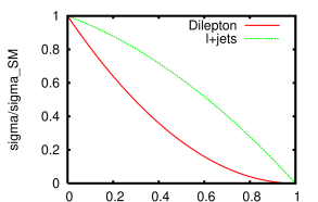
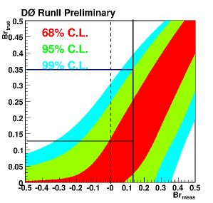
Figure 5: Left: Expected dilepton and $\ell+$jets reduction as function of top branching fraction to leptophobic charged Higgs. Right: Confidence intervals in the measured vs. nominal $B$ plane.

Assuming a leptophobic charged Higgs, i.e. $B(H^{\pm}\rightarrow cs)=100\%$, dileptonic events can only appear if both top quarks decay through a $W$ boson. In $\ell+$jets events at least one top decay must occur through a $W$ boson. The higher the contribution of top decays through charged Higgs the less likely is the decay through a $W$ boson. Thus both channels will have a reduced contribution with respect to the SM. However, the reduction is stronger in the dilepton channel, see Fig. 5 (left). The cross-section ratio dependence can be written as

$$R_{\sigma}=1+\frac{x}{(1-x)B(W\rightarrow qq)}\quad\mbox{with}\quad x=B(t\rightarrow H^{\pm}b)\mbox{.}$$ (1)

As an extention to this formula the actual analysis accounts for leakage between the channels. With this the above result on $R_{\sigma}$ can be converted to a limit on the charged Higgs contribution in top decays. As before ensembles of results for various nominal values of $B(t\rightarrow H^{\pm}b)$ were generated with appropriate treatment of systematic uncertainties. Then the Feldman-Cousins approach is used to determine the final result accounting for the physical constraints of $0\leq B(t\rightarrow H^{\pm}b)\leq 1$. D0 finds $B(t\rightarrow H^{\pm}b)<0.35$ at 95% confidence level. Because the measured $R_{\sigma}$ is slightly larger than 1 the expected limit of $B(t\rightarrow H^{\pm}b)<0.25$ is not reached.

4 Search for Exotic Top Charge

The top quark’s electrical properties are fixed by its charge. However, in reconstructing top quarks the charges of the objects usually aren’t checked. Thus an exotic charge value of $\left|q_{t}\right|=4e/3$ isn’t excluded by standard analyses. To distinguish between the SM and the exotic top charge it is necessary to reconstruct the charges of the top quark decay products, the $W$ boson and the $b$ quark. The $W$ boson charge can be taken from the charge of the reconstructed lepton, but finding the charge of the $b$ quark is more difficult.

4.1 Data Selection and Background Description

D0 has performed an analysis of $\ell+$jets events with at least to $b$-tagged jets in $370\,\mbox{fb}^{-1}$ using a jet charge technique to determine the charge of the $b$ jets [7]. Semileptonic events are selected following the cross-section analysis by requiring exactly one isolated lepton, tranverse missing energy and 4 or more jets. At least 2 of the jets must be identified as $b$ jets using a secondary vertex tagging algorithm.

4.2 Jet Charge

The charge of a jet can be defined as the sum of the charges of all tracks inside the cone of that jet. In this analysis the sum has been weighted with the tracks transverse momentum:

$$Q_{\mathrm{jet}}:=\frac{\sum{q_{i}\cdot p^{0.6}_{Ti}}}{\sum{p^{0.6}_{Ti}}}$$ (2)

Because particles may easily escape the jet cone such a jet charge fluctuates strongly from event to event, only statistical statements can be made. It is crucial to determine the expected distribution of $Q_{\mathrm{jet}}$ in the case of $b$ or $\bar{b}$ quark and, because a significant fraction of charm quarks gets flagged by the secondary vertex tagger, also for the $c$ and $\bar{c}$ quarks. These expected distributions, c.f. Fig. 6 (left), are derived from dijet data using a tag and probe method.

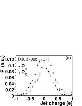
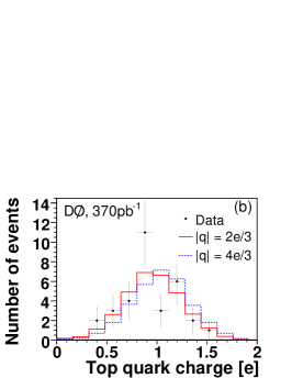
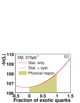
Figure 6: Expected jet charge distribution for $b$ and anti-$b$ quarks (left). Measured absolute top charge compared to SM and exotic models (middle). Likelihood as function of the fraction of exotic top quarks (right).

4.3 Top Charge Results

To determine the top charge an assignment of $b$-jets to the leptonic or hadronic event side is necessary. This analysis uses the quality of a fit to the $t\bar{t}$ hypothesis, which uses the $W$ and top masses as constraints, to select the best possible assignment. The jet charge for the $b$ jets for the leptonic (hadronic) side, $q_{b_{l}}$ ($q_{b_{h}}$) is then combined with the charge of the measured lepton $q_{l}$ to define two top charge values per event: $Q_{\mathrm{lep}}=\left|q_{l}+q_{b_{\mathrm{l}}}\right|$ and $Q_{\mathrm{had}}=\left|-q_{l}+q_{b_{\mathrm{h}}}\right|$. The distribution of the measured top charges is compared to MC templates for the SM and the exotic case, where the exotic case has been obtained by permuting the jet charge, see Fig. 6 (middle).

An unbinned likelihood ratio accounting also for remaining background yields a $p$-value for the exotic case of $7.8\%$ and a Bayes factor of 4.3.

5 Search for Top Pair Resonances

Due to the fast decay of the top quark, no resonant production of top pairs is expected within the SM. However, unknown heavy resonances decaying to top pairs may add a resonant part to the SM production mechanism. Resonant production is possible for massive $Z$-like bosons in extended gauge theories [8], Kaluza-Klein states of the gluon or $Z$ boson [9, 10], axigluons [11], Topcolor [12], and other theories beyond the SM. Independent of the exact model, such resonant production could be visible in the reconstructed $t\bar{t}$ invariant mass.

5.1 Data Selection, Signal and Background Description

D0 investigated the invariant mass distribution of top pairs in $2.1\,\mbox{fb}^{-1}$ of $\ell+$jets events[13, 14]. The event selection and background description follow closely the description in section 2.1, with the exception that also events with only three jets are considered. Signal simulation is created for various resonance masses between $350$ and $1000\,\mbox{Ge\kern-0.86108ptV}$. The width of the resonances was chosen to be $1.2\%$ of their mass, which is much smaller than the detector resolution.

5.2 Top Pair Invariant Mass

The top pair invariant mass, $M_{t\bar{t}}$, is reconstructed directly from the reconstructed physics objects. A constraint fit as described in 2.1 is not applied. Instead the momentum of the neutrino is reconstructed from the transverse missing energy, $/\!\!\!\!{E_{T}}$, which is identified with the transverse momentum of the neutrino and by solving $M_{W}^{2}=(p_{\ell}+p_{\nu})^{2}$ for the $z$-component of the neutrino momentum. $p_{\ell}$ and $p_{\nu}$ are the four-momenta of the lepton and the neutrino, respectively.

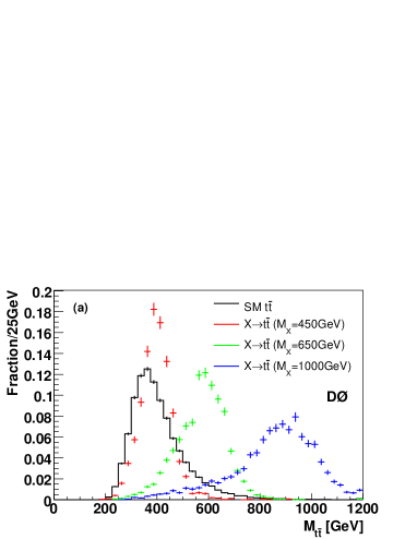
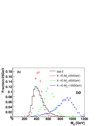
Figure 7: Shape comparison of the expected $t\bar{t}$ invariant mass distributions for SM top quark pair production (histogram) and resonant production from narrow-width resonances of mass $M_{X}=450$, $650$, and $1000\,\mbox{Ge\kern-0.86108ptV}$, for (a) $3$ jets events and (b) $\geq 4$ jets events.

The $t\bar{t}$ invariant mass can then be computed without any assumptions about a jet-parton assignments that is needed in constraint fits. Compared to the constraint fit reconstruction applied in earlier analysis this gives better performance at high resonance masses and in addition allows the inclusion of $\ell+$3 jets events. The expected signal shapes for various resonance masses are compared to the SM top pair distribution in Fig. 7. The expected distribution of SM processes and the measured data is shown in Fig. 8. For comparison a $Z^{\prime}$ resonance with a mass of $650\,\mbox{Ge\kern-0.86108ptV}$ is shown at the cross-section expected in the topcolor assisted technicolor model used for reference.

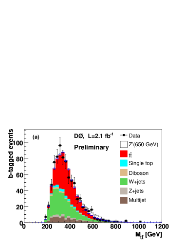
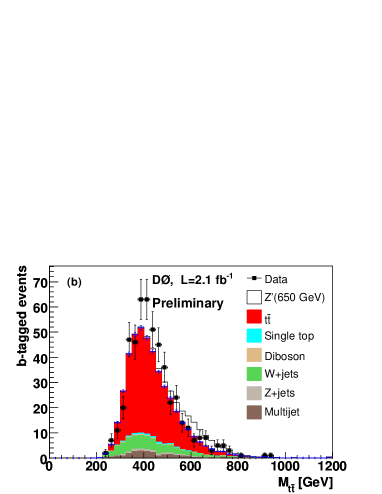
Figure 8: Expected and observed $t\bar{t}$ invariant mass distribution for the combined (a) $\ell+3$ jets and (b) $\ell+4$ or more jets channels, with at least one identified $b$ jet. Superimposed as white area is the expected signal for a Topcolor-assisted technicolor $Z^{\prime}$ boson with $M_{Z^{\prime}}=650\,\mbox{Ge\kern-0.86108ptV}$.

5.3 Limit Calculation and Systematics

Cross-section for resonant production are evaluated using the Bayesian technique described in 2.3. Central values correspond to the maximum of the posterior probability density, limits are set at the point where the integral of the posterior probability density from zero reaches $95\%$ of its total. Expected limits are obtained by applying the procedure when assuming that the observed result corresponded to the SM expectation.

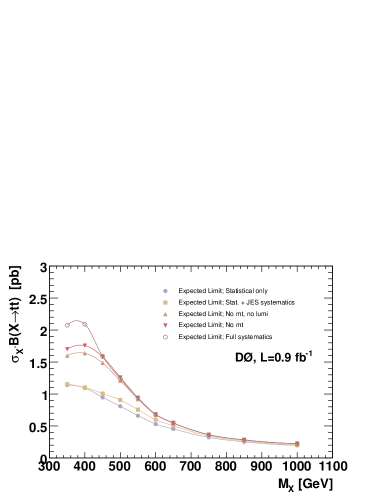
Figure 9: Expected limits (from bottom to top) without systematics, including only JES systematics, excluding selection efficiencies, $m_{t}$ and luminosity, all except $m_{t}$ and complete systematics.

These expected limits were used to optimise major analysis cut and the $b$-tag working point. In Fig. 9 the expected limits are used to visualise the effect of the various systematics by including one after another. The lowest curve corresponds to a purely statistical limit. Adding the jet energy uncertainty shows that this uncertainty mainly contributes at medium resonance masses. The various object identification efficiencies and the luminosity are added. They essentially scale like the background shape. Finally the effect of the top mass is shown and it is most important at low resonance masses.

5.4 Results

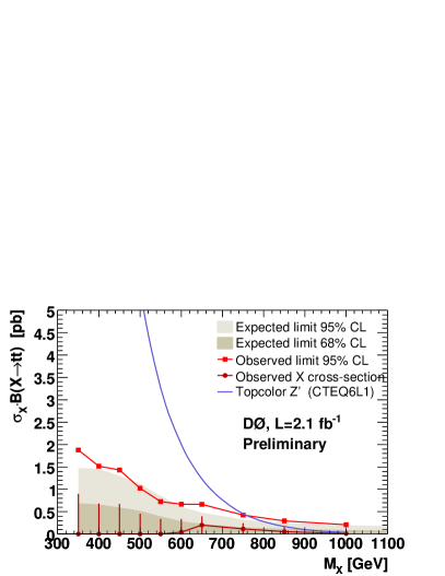
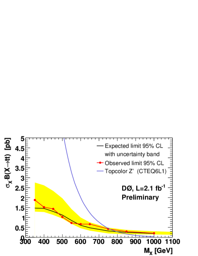
Figure 10: Left: Expected upper limits on $\sigma_{X}\cdot B(X\rightarrow t\bar{t})$ (shaded) vs. the assumed resonance mass compared to the observed cross-section and exclusion limits at 95%CL. Right: Expected limit with 1$\sigma$ uncertainty band compared to observed result. Both figures show the prediction of the topcolor assisted technicolor model used to derive benchmark mass limits.

The observed cross-sections are close to zero for all considered resonance masses, as shown Fig. 10 (left). The largest deviation (around $700\,\mbox{Ge\kern-0.86108ptV}$) is about one standard deviation. Thus limits are set on the $\sigma_{X}\cdot B(X\rightarrow t\bar{t})$ as function of the assumed resonance mass, $M_{X}$. The excluded values range from less than about $2\,\mbox{pb}$ for low mass resonances to less then $0.21\,\mbox{pb}$ for the highest considered resonance mass of $1\,\mbox{Te\kern-0.86108ptV}$. The benchmark topcolor assisted technicolor model can be excluded for resonance masses of $M_{Z^{\prime}}<760\,\mbox{Ge\kern-0.86108ptV}$ at $95\%$CL.

6 Summary

D0 has searched for signs of physics beyond the standard in top pair production signatures in various aspects of top quark production, properties and decays. In datasets of up to $2.1\,\mbox{fb}^{-1}$ no deviation from the standard model of elementary particle physics was found.

References

- [1] \NAMEAbe F. et al., \INPhys. Rev. Lett. 7419952626.
- [2] \NAMEAbachi S. et al., \INPhys. Rev. Lett. 7419952632.
- [3] \NAMEJabeen S., \TITLEMeasurements of single top at D0, in these proceedings.
- [4] \NAMEShabalina E., \TITLEMeasurement of top properties at D0, in these proceedings.
- [5] \NAMEAbazov V. M. et al., \TITLESearch for scalar top admixture in the lepton+jets final state at in of DØ data, D0 Note 5438 Conf (2007).
- [6] \NAMEAbazov V. M. et al., \TITLEMeasurement of the cross section ration with the D0 detector at in the Run II data, D0 Note 5466 conf (2007).
- [7] \NAMEAbazov V. M. et al., \INPhys. Rev. Lett. 982007041801.
- [8] \NAMELeike A., \INPhys. Rept. 3171999143.
- [9] \NAMELillie B., Randall L. \atqueWang L.-T., \INJHEP 092007074.
- [10] \NAMERizzo T. G., \INPhys. Rev. D 612000055005.
- [11] \NAMESehgal L. M. \atqueWanninger M., \INPhys. Lett. B 2001988211.
- [12] \NAMEHill C. T. \atqueParke S., \INPhys. Rev. D 4919944454.
- [13] \NAMEAbazov V. M. et al., \TITLESearch for resonances in the lepton plus jets final state in collisions at , arXiv:0804.3664 [hep-ex] (2008).
- [14] \NAMEAbazov V. M. et al., \TITLESearch for resonances in the lepton+jets final state in collisions at , D0 Note 5600 conf (2008).