DESY 08-084
PITHA-08/14 Virtual Hadronic Corrections to Massive Bhabha Scattering

Abstract

Virtual hadronic contributions to the Bhabha process at the NNLO level are discussed. They are substantial for predictions with per mil accuracy. The studies of heavy fermion and hadron corrections complete the calculation of Bhabha virtual effects at the NNLO level.

1 Introduction

Since Loops and Legs 2006 [1, 2], considerable progress in the determination of the virtual NNLO corrections to the massive QED Bhabha process has been made .

The $N_{f}=2$ two-loop corrections with heavy-fermion insertions have been computed in the limit $m_{e}^{2}<<m_{f}^{2}<<s,t$: with a direct Feynman diagram calculation in [15], and using a factorization formula that relates massless and massive amplitudes in [16].

Hadronic contributions have been recently calculated in [17]. In addition, heavy-fermion corrections, beyond the $m_{f}^{2}<<s,t$ limit, have been made available in [17, 18, 19]; see also [20].

Interestingly, the original expectations on the necessity of a complete, direct two-loop massive Feynman diagram evaluation have not been fulfilled yet. After the analytical evaluation of a massive planar and a massive non-planar double-box diagram (both with seven propagators) in [21] and in [22], there was hope to evaluate all the remaining diagrams soon [23]. So far only part of the photonic master integrals, namely the planar ones, have been evaluated in [24] in the limit of small electron mass. Although this limit is by far sufficient for experiments, there is still space for theoretical developments.

Finally, it should be stressed that results for three gauge-invariant classes of NNLO Feynman diagrams have been determined by at least two independent groups, relying on different methods:

• Photonic corrections: computed in [12, 13] and recalculated in [16];

• Electron $N_{f}=1$ corrections: computed in [10] and cross-checked in [15] (with full $m_{e}$ dependence) and in [16] (small electron mass limit);

• Heavy-fermion $N_{f}=2$ contributions: determined with two independent methods in the limit $m_{f}^{2}<<s,t$ in [15, 16] and for any mass $m_{f}$ in [25, 17] (dispersive approach) and in [18, 19] (analytical result).

As far as the full electroweak model is concerned, the NLO corrections are well known [26, 27]. At NNLO, the terms enhanced by the heavy top quark are taken into account [28, 29]. The full dependence of weak corrections on the top quark and Higgs boson masses is known [30, 31] and implemented for fermion pair production in $e^{+}e^{-}$-annihilation [32], but is not yet implemented for Bhabha scattering. Here, we report on another class of NNLO corrections, which have recently determined:

• Virtual hadronic NNLO contributions, including both reducible self-energy insertions and irreducible vertex and box corrections [17].

For a review on the status of Monte Carlo studies for Bhabha scattering we refer to [33].

2 Hadronic Virtual Corrections

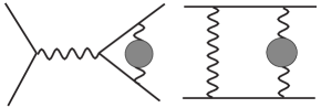
Figure 1: Two-loop irreducible vertex and box topologies for Bhabha scattering with vacuum polarization insertions.

Higher order hadronic corrections to the Bhabha scattering cross section can be obtained inserting the renormalized irreducible photon vacuum polarization function, $\Pi$, in the appropriate virtual-photon propagator (see Fig. 1),

$$\frac{g_{\mu\nu}}{q^{2}\!+\!i\delta}\!\to\!\frac{g_{\mu\alpha}}{q^{2}\!+\!i\delta}\left(q^{2}g^{\alpha\beta}\!-\!q^{\alpha}q^{\beta}\right)\Pi(q^{2})\frac{g_{\beta\nu}}{q^{2}\!+\!i\delta},$$ (1)

where $q$ is the momentum carried by the virtual photon and $\delta\to 0_{+}$. The vacuum polarization function $\Pi$ can be represented by the once-subtracted dispersion integral [34],

$$\Pi(q^{2})=-\frac{q^{2}}{\pi}\,\int_{4M^{2}}^{\infty}\,dz\,\frac{\text{Im}\,\Pi(z)}{z}\,\frac{1}{q^{2}-z+i\,\delta},$$ (2)

where the production threshold for the intermediate state in $\Pi$ is located at $q^{2}=4M^{2}$. We leave as understood the subtraction at $q^{2}=0$ for the renormalized photon self-energy.

Light-quark contributions get modified by low-energy strong-interaction effects, which cannot be computed using perturbative QCD. However, these contributions can be evaluated using the optical theorem [35], and relating $\text{Im}\,\Pi_{\rm had}$ to the hadronic cross-section ratio $R_{\rm had}$ [34],

$$\text{Im}\,\Pi_{\rm had}(z) = -\frac{\alpha}{3}\,R_{\rm had}(z),$$ (3)

$$R_{\rm had}(z) = \frac{\sigma(\{e^{+}e^{-}\to\gamma^{\star}\to\text{hadrons}\};z)}{(4\pi\alpha^{2})/(3z)}.$$

$\text{Im}~{}\Pi_{\rm had}$ can be computed employing the experimental data for $R_{\rm had}$ in the low-energy region and around hadronic resonances, and the perturbative-QCD prediction in the remaining regions.

Here we give numerical results through tables which have been included also in the first version of [36].

A shape of the $R_{had}$ parameterization we use is given in Fig. 2. In a forthcoming publication [38], containing a detailed description of [17], we will employ a more updated parameterization of $R_{had}$ [39, 40, 41]. We just mention that the final numbers get modified only slightly and do not change qualitatively the situation.

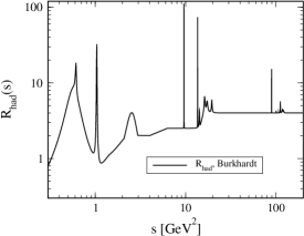
Figure 2: $R_{had}(s)$, based on the parameterization given in [42].

The lower integration boundary in Eq. (2) is given by $M=m_{\pi}$, where $m_{\pi}$ is the pion mass. For self-energy corrections to Bhabha scattering at one-loop order this method was first employed in [43].

Finally, we note that contributions to $\Pi$ arising from leptons and the top quark can be computed directly in perturbation theory, setting $M=m_{f}$ in Eq. (2), where $m_{f}$ is the mass of the fermion appearing in the loop, and inserting the imaginary part of the analytic result for $\Pi$.

In the following, we will not consider hadronic effects to the running of the coupling constant; details can be found in [38].

3 Vertex Contributions

Hadronic irreducible vertex corrections are obtained through the interference of the vertex diagrams of Figure 1 with the tree-level amplitude. Their contribution to the ${\cal O}(\alpha^{4})$ differential cross section is given by:

$$\frac{d\sigma_{\rm vert}}{d\Omega} = 4\left(\frac{\alpha}{\pi}\right)^{2}\,\left(\frac{\,\alpha^{2}}{2s}\right)$$

$$\times \Bigl{\{}\frac{v_{1}(s,t)}{s^{2}}\text{Re}V_{2}(s)+\frac{v_{1}(t,s)}{t^{2}}V_{2}(t)$$

$$+ \frac{v_{2}(s,t)}{s,t}\Bigl{[}\text{Re}V_{2}(s)+V_{2}(t)\Bigr{]}\Bigl{\}}+{\cal O}(m_{e}^{2}),$$

where we define $v_{1}(x,y)=x^{2}+2y^{2}+2xy$ and $v_{2}(x,y)=(x+y)^{2}$). Here $V_{2}$ summarizes all two-loop fermionic corrections to the QED Dirac form factor, whose computation can be traced back to the seminal work of [44, 45]. The full result can be organized as

$$V_{2}(x) = V_{2e}(x)+V_{2{\rm rest}}(x),$$ (6)

where $V_{2e}$ denotes the electron-loop component, see [46].

Heavy-fermion and hadronic contributions, instead, can be evaluated as in Ref. [47] through the dispersion integral

$$V_{2{\rm rest}}(x)=\int_{4M^{2}}^{\infty}\,dz\,\frac{R(z)}{z}\,K_{V}(x+i\delta;z),$$ (7)

where $R$ is given by

$$R(z) = R_{\rm had}^{(5)}(z)-\frac{3}{\alpha}\,\sum_{f=e,\mu,\tau,t}\,\text{Im}\,\Pi_{f}(z)$$

$$= R_{\rm had}^{(5)}(z)+\sum_{f=e,\mu,\tau,t}R_{f}(z;m_{f}),$$

$$R_{f}(z;m_{f}) = Q_{f}^{2}C_{f}\left(1+\frac{2m_{f}^{2}}{z}\right)\sqrt{1-\frac{4m_{f}^{2}}{z}},$$

and where $C_{f}$ and $Q_{f}$ denote the color factor and the electric charge. The two-loop irreducible vertex kernel function $K_{V}$, in the limit of a vanishing electron mass, reads as:

$$K_{V}(x;z) = \frac{1}{3}\Bigl{\{}-\frac{7}{8}-\frac{z}{2x}+\Bigl{(}\frac{3}{4}\!+\!\frac{z}{2x}\Bigr{)}\ln\frac{-x}{z}$$

$$- \frac{1}{2}\Bigl{(}1\!+\!\frac{z}{x}\Bigr{)}^{2}\Bigl{[}\zeta_{2}\!-\!\text{Li}_{2}\left(1\!+\!\frac{x}{z}\right)\Bigr{]}\Bigr{\}}.$$

Here $\text{Li}_{2}$ is the usual dilogarithm and $\zeta_{2}={\rm{Li_{2}}}(1)=\pi^{2}/6$.

In Tables 1 and  2 we show numerical values for the various components of $V_{2}(x)$ of Eq. (6) for space-like and time-like values of $x$ ($t$ and $s$ channel). For each fermion flavour, we show the result obtained through the dispersion-based approach (first line) and the one coming from the analytical expansion (second line).

We can see that the latter numbers approach the former ones in regions where the analytical expansions are expected to become good approximations. When $m_{f}^{2}>s$, the entry is suppressed.

$\theta=3^{\circ}$  $|$   $\sqrt{s}$	1 GeV	10 GeV	$M_{Z}$	500 GeV
$e$	-5.880	-28.47	-80.91	-151.0
$\mu$	-0.005	-0.20	-2.85	-11.8
	$\times$	1.04	-2.78	-11.8
$\tau$	$<$ 10-3	$<$ 10-2	-0.08	-0.8
	$\times$	$\times$	2.26	-0.5
$t$		$<$ 10-2	$<$ 10-2	$<$ 10-1
	$\times$	$\times$	$\times$	$\times$
had.	-0.004	-0.20	-4.08	-21.5
$\theta=90^{\circ}$  $|$   $\sqrt{s}$	1 GeV	10 GeV	$M_{Z}$	500 GeV
$e$	-47.44	-122.2	-246.6	-386.7
$\mu$	-0.74	-7.4	-31.4	-70.6
	-0.36	-7.4	-31.4	-70.6
$\tau$	-0.01	-0.4	-4.4	-16.2
	$\times$	0.3	-4.4	-16.2
$t$		$<$ 10-1	$<$ 10-1	-0.2
	$\times$	$\times$	$\times$	1.8
had.	-0.87	-12.5	-67.6	-172.2

Table 1: Contributions to $V_{2}$ in the $t$ channel for two values of the scattering angle, $\theta=3^{\circ}$ and $\theta=90^{\circ}$, $t=-s\,\sin^{2}(\theta/2)$.

4 Box Contributions

Notice that, unlike the vertex kernel, the irreducible box kernels are infrared divergent, but, analogously to the one-loop box diagrams, they have no singularity in the electron mass . In order to construct an infrared-finite quantity, we combine: (i) Born diagrams interfering with two-loop box diagrams and reducible vertices (first row in Fig. 3); (ii) diagrams with a one-loop vacuum polarization insertion interfering with one-loop boxes and vertices (second row in Fig. 3); (iii) real single-photon emission diagrams with a one-loop vacuum polarization insertion (third row in Fig. 3). The infrared-safe $N_{f}=2$ irreducible vertices (see Fig. 1) and pure self-energy diagrams are not included here.

The resulting cross-section becomes

$$\frac{d\overline{\sigma}}{d\Omega}=c\int_{4M_{\pi}^{2}}^{\infty}dz\frac{R_{\mathrm{had}}(z)}{z}\frac{1}{t-z}F_{1}(z)$$ (10)

$$+ c\int_{4M_{\pi}^{2}}^{\infty}\frac{dz}{z\left(s-z\right)}\Bigl{\{}R_{\mathrm{had}}(z)\Bigl{[}F_{2}(z)$$

$$+ F_{3}(z)\ln\bigl{|}1-\frac{z}{s}\bigr{|}\Bigr{]}-R_{\mathrm{h}}(s)\Bigl{[}F_{2}(s)$$

$$+ F_{3}(s)\ln\bigl{|}1-\frac{z}{s}\bigr{|}\Bigr{]}\Bigr{\}}+c~{}\frac{R_{\mathrm{h}}(s)}{s}\times$$

$$\Bigl{\{}F_{2}(s)\ln\Bigl{(}\frac{s}{4M_{\pi}^{2}}-1\Bigr{)}-6\zeta_{2}F_{a}(s)$$

$$+ F_{3}(s)\Bigl{[}2\zeta_{2}+\frac{1}{2}\ln^{2}\Bigl{(}\frac{s}{4M_{\pi}^{2}}-1\Bigr{)}$$

$$+ \text{Li}_{2}\Bigl{(}1-\frac{s}{4M_{\pi}^{2}}\Bigr{)}\Bigr{]}\Bigr{\}},$$

with $c=\alpha^{4}/(\pi^{2}s)$. The $F_{1,2,3}$ and $F_{a}$ are defined as in [17] and [37], and $R_{\mathrm{h}}(s)=\theta(s-4M_{\pi}^{2})~{}R_{\mathrm{had}}(s)$.

Numerical results are given in Tables 3 and 4, where we include also the QED Born prediction, the Standard Model effective Born prediction for $M_{Z}=91.188\mathrm{~{}GeV}$, $\Gamma_{Z}=2.495\mathrm{~{}GeV}$, $\sin^{2,eff}_{W}=0.23$ and the contribution from the running of the fine-structure constant. The cut on the energy of the soft photons is set to $\sqrt{s}/2$. We can see that, refering to the per mil accuracy: (i) electron vertices dominate over the rest of vertices (however, it is known that they largely cancel with the contribution of the soft electron pair emission of [3], see also [38]); (ii) contributions from infrared-safe boxes in Eq. 10 are substantial, mostly due to the factorizing diagrams; (iii) hadronic contributions play an important role.

$\sqrt{s}$	1 GeV	10 GeV	$M_{Z}$	500 GeV
$e$	-45.87	-124.2	-254.4	-400.6
$\mu$	0.36	-4.8	-29.1	- 70.1
	0.21	-4.8	-29.1	-70.1
$\tau$	0.02	0.3	-2.1	-13.5
	$\times$	0.1	-2.1	-13.5
$t$		$<$ 10-1	$<$ 10-1	0.3
	$\times$	$\times$	$\times$	$<$ 10-1
had.	0.92	-4.8	-57.1	-165.3

Table 2: Contributions to Re $V_{2}$ in the $s$ channel. See Table 1 for further details.

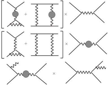
Figure 3: IR divergent contributions, becoming finite after combining with irreducible boxes.

5 Summary

Virtual NNLO QED corrections to massive Bhabha scattering have been completed in the small electron mass limit. Photonic, electron and heavy-fermion contributions have been checked by independent groups and different methods of calculations. Hadronic contributions have been calculated through the dispersion relation approach; the kernels employed have been checked through a comparison with the heavy-fermion result of [18, 19].

The analysis of the virtual NNLO contributions shows that the results can influence Bhabha physics; therefore, further studies including Monte Carlo calculations with real bremsstrahlung are welcome [33].

$\sqrt{s}$ [GeV]	1	10	$M_{Z}$	500
QED Born	440994	4409.94	53.0348	1.76398
ew. Born	440994	4409.95	53.0370	1.76331
self energies (A)	445283	4495.45	55.5352	1.90910
irred. vertices (B)	-56	-2.74	-0.1005	-0.00704
boxes+red. (C)  $e$	193	5.73	0.1357	0.00673
$\mu$	$<$ 1	0.42	0.0408	0.00288
	$-$	0.08	0.0407	0.00288
$\tau$	$<$ 1	$<$ 10-2	0.0027	0.00088
	$-$	$-$	-0.0096	0.00084
$t$	$<$ 1	$<$ 10-2	$<$ 10-4	$<$ 10-5
	$-$	$-$	$-$	$-$
had	$<$ 1	0.39	0.0877	0.00811
$\sum_{\rm{boxes+red.}}$ (C)	193	6.54	0.2669	0.01860
$\mathrm{A+B+C}$	445420	4499.25	55.7016	1.92066

Table 3: Differential cross sections in nanobarns at a scattering angle $\theta=3^{\circ}$, in units of $10^{2}$. A – QED $\alpha$ running [48]; B – irreducible vertex corrections, C – net sum of infrared-sensitive corrections, including double boxes, dispersion approach (first line) and analytical expansion [15] (second line). When $m_{f}^{2}>s,|t|,|u|$, the entry is suppressed. Parameters: $\omega=\sqrt{s}/2$, $M_{Z}$ = 91.1876 GeV, $m_{t}$=172.5 GeV.

$\sqrt{s}$ [GeV]	1	10	$M_{Z}$	500
QED Born	466537	4665.37	56.1067	1.86615
ew. Born	466558	4686.27	1289.3011	0.85496
self energies (A)	480106	4984.83	62.9027	2.17957
irred. vertices (B)	-494	-14.35	-0.4239	-0.02602
boxes + red. (C) $e$	807	14.53	0.2706	0.01193
$\mu$	160	6.08	0.1470	0.00726
	153	6.08	0.1470	0.00726
$\tau$	2	1.33	0.0752	0.00457
	$-$	1.07	0.0752	0.00457
$t$	$<$ 1	$<$ 10-2	0.0005	0.00043
	$-$	$-$	$-$	-0.00013
had.	234	16.07	0.4701	0.02461
$\sum_{\rm{boxes+red.}}$ (C)	1203	38.01	0.9634	0.04880
$\mathrm{A+B+C}$	480815	5008.49	63.4422	2.20235

Table 4: The same as in Tab. 3, at a scattering angle $\theta=90^{\circ}$, in units of $10^{-4}$.

References

- [1] J. Blümlein, S. Moch and T. Riemann, Proc. of 8th DESY Workshop on Elementary Particle Theory “Loops and Legs in Quantum Field Theory”, Eisenach, Germany, 23-28 April 2006, Nucl. Phys. Proc. Suppl. 160 (2006) 1.
- [2] S. Actis et al., Nucl. Phys. Proc. Suppl. 160 (2006) 91, hep-ph/0609051.
- [3] A. Arbuzov et al., Phys. Atom. Nucl. 60 (1997) 591.
- [4] A. Arbuzov, E. Kuraev and B. Shaikhatdenov, Mod. Phys. Lett. A13 (1998) 2305, hep-ph/9806215.
- [5] Z. Bern, L. Dixon and A. Ghinculov, Phys. Rev. D63 (2001) 053007, hep-ph/0010075.
- [6] N. Glover, B. Tausk and J. van der Bij, Phys. Lett. B516 (2001) 33, hep-ph/0106052.
- [7] R. Bonciani et al., Nucl. Phys. B681 (2004) 261, hep-ph/0310333.
- [8] M. Czakon, J. Gluza and T. Riemann, Nucl. Phys. Proc. Suppl. 135 (2004) 83, hep-ph/0406203.
- [9] M. Czakon, J. Gluza and T. Riemann, Phys. Rev. D71 (2005) 073009, hep-ph/0412164.
- [10] R. Bonciani et al., Nucl. Phys. B701 (2004) 121, hep-ph/0405275.
- [11] R. Bonciani et al., Nucl. Phys. B716 (2005) 280, hep-ph/0411321v2.
- [12] A. Penin, Phys. Rev. Lett. 95 (2005) 010408, hep-ph/0501120.
- [13] A. Penin, Nucl. Phys. B734 (2006) 185, hep-ph/0508127.
- [14] R. Bonciani and A. Ferroglia, Phys. Rev. D72 (2005) 056004, hep-ph/0507047.
- [15] S. Actis et al., Nucl. Phys. B786 (2007) 26, arXiv:0704.2400v.2 [hep-ph].
- [16] T. Becher and K. Melnikov, JHEP 06 (2007) 084, arXiv:0704.3582 [hep-ph].
- [17] S. Actis et al., Phys. Rev. Lett. 100 (2008) 131602, arXiv:0711.3847.
- [18] R. Bonciani, A. Ferroglia and A.A. Penin, Phys. Rev. Lett. 100 (2008) 131601.
- [19] R. Bonciani, A. Ferroglia and A.A. Penin, JHEP 02 (2008) 080, arXiv:0802.2215.
- [20] R. Bonciani, these proceedings.
- [21] V. Smirnov, Phys. Lett. B460 (1999) 397, hep-ph/9905323.
- [22] B. Tausk, Phys. Lett. B469 (1999) 225, hep-ph/9909506.
- [23] G. Heinrich and V. Smirnov, Phys. Lett. B598 (2004) 55, hep-ph/0406053.
- [24] M. Czakon, J. Gluza and T. Riemann, Nucl. Phys. B751 (2006) 1, hep-ph/0604101.
- [25] S. Actis et al., Acta Phys. Polon. B38 (2007) 3517, arXiv:0710.5111 [hep-ph].
- [26] M. Consoli, Nucl. Phys. B160 (1979) 208.
- [27] M. Bohm, A. Denner and W. Hollik, Nucl. Phys. B304 (1988) 687.
- [28] D. Bardin, W. Hollik and T. Riemann, Z. Phys. C49 (1991) 485.
- [29] D. Bardin et al., Comput. Phys. Commun. 133 (2001) 229, hep-ph/9908433.
- [30] M. Awramik et al., Phys. Rev. D69 (2004) 053006, hep-ph/0311148.
- [31] M. Awramik, M. Czakon and A. Freitas, JHEP 11 (2006) 048, hep-ph/0608099.
- [32] A. Arbuzov et al., Comput. Phys. Commun. 174 (2006) 728, hep-ph/0507146.
- [33] G. Montagna, these proceedings.
- [34] N. Cabibbo and R. Gatto, Phys. Rev. 124 (1961) 1577.
- [35] R.E. Cutkosky, J. Math. Phys. 1 (1960) 429.
- [36] S. Actis et. al., arXiv:0711.3847v1 [hep-ph].
-
[37]
DESY, webpage http://www-zeuthen.desy.de
/theory/research/bhabha/bhabha.html. - [38] S. Actis et. al., to be submitted.
- [39] K. Hagiwara et al., Phys. Lett. B557 (2003) 69, hep-ph/0209187.
- [40] K. Hagiwara et al., Phys. Rev. D69 (2004) 093003, hep-ph/0312250.
- [41] K. Hagiwara et al., Phys. Lett. B649 (2007) 173, hep-ph/0611102.
- [42] H. Burkhardt, TASSO-NOTE-192 (1981), and Fortran program repi.f (1986).
- [43] F. Berends and G. Komen, Phys. Lett. B63 (1976) 432.
- [44] R. Barbieri, J.A. Mignaco and E. Remiddi, Nuovo Cim. A11 (1972) 824.
- [45] R. Barbieri, J.A. Mignaco and E. Remiddi, Nuovo Cim. A11 (1972) 865.
- [46] G. Burgers, Phys. Lett. B164 (1985) 167.
- [47] B. Kniehl et al., Phys. Lett. B209 (1988) 337.
- [48] S. Eidelman and F. Jegerlehner, Z. Phys. C67 (1995) 585, hep-ph/9502298.