Sets of non-differentiability for conjugacies between expanding interval maps

Abstract.

We study differentiability of topological conjugacies between expanding piecewise $C^{1+\epsilon}$ interval maps. If these conjugacies are not $C^{1}$, then they have zero derivative almost everywhere. We obtain the result that in this case the Hausdorff dimension of the set of points for which the derivative of the conjugacy does not exist lies strictly between zero and one. Using multifractal analysis and thermodynamic formalism, we show that this Hausdorff dimension is explicitly determined by the Lyapunov spectrum. Moreover, we show that these results give rise to a “rigidity dichotomy” for the type of conjugacies under consideration.

1. Introduction and statement of results

In this paper we study aspects of non-differentiability for conjugacy maps between certain interval maps. The maps under consideration are called expanding piecewise $C^{1+\epsilon}$ maps. These are expanding maps of the unit interval $\mathcal{U}$ into itself which have precisely $d$ increasing full inverse branches and each of these branches is a $C^{1+\epsilon}$ diffeomorphism on $\mathcal{U}$, for some fixed $\epsilon>0$ and some fixed integer $d\geq 2$ (a map $f:\mathcal{U}\to f\left(\mathcal{U}\right)\subset{\mathbb{R}}$ is said to be a $C^{1+\epsilon}$ diffeomorphism if there exists an extension $\widetilde{f}$ of $f$ to some open neighbourhood of $\mathcal{U}$ which is a diffeomorphism such that $\widetilde{f}^{\prime}|_{\mathcal{U}}$ is Hölder continuous with Hölder exponent equal to $\epsilon$). Clearly, each expanding piecewise $C^{1+\epsilon}$ map is naturally semi-conjugate to the full shift $\Sigma$ over the alphabet $A:=\left\{1,\ldots,d\right\}$. Moreover, for two maps $S$ and $T$ of this type the following diagram commutes, where $\sigma$ refers to the usual shift map on $\Sigma$, and $\pi_{S}$ and $\pi_{T}$ denote the associated coding maps.

$$\begin{CD}\mathcal{U}@<{\pi_{T}}<{}<\Sigma @>{\pi_{S}}>{}>\mathcal{U}\\ @V{T}V{}V@V{}V{\sigma}V@V{}V{S}V\\ \mathcal{U}@<{\pi_{T}}<{}<\Sigma @>{\pi_{S}}>{}>\mathcal{U}\end{CD}$$

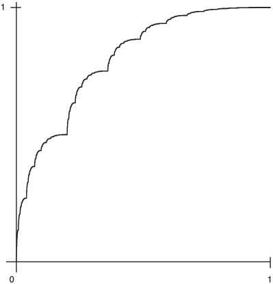
(a) $\tau=1/5$

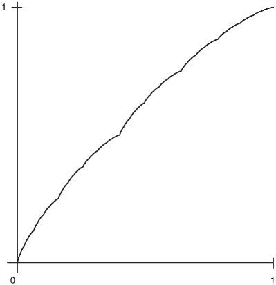
(b) $\tau=2/5$

Figure 1. The conjugating map $\Theta_{\tau}$ for the Salem case.

The conjugacy map $\Theta:\mathcal{U}\to\mathcal{U}$ between the two systems $(\mathcal{U},S)$ and $(\mathcal{U},T)$ is then given by $T\circ\Theta=\Theta\circ S$ (see Fig. 1 and 4 for some examples). The first main result of the paper will be to employ the thermodynamic formalism in order to give a detailed fractal analysis of the following three sets:

$$\mathcal{D}_{\sim} = \mathcal{D}_{\sim}(S,T):=\{\xi\in\mathcal{U}:\Theta^{\prime}(\xi)\mbox{ does not exists in the generalised sense}\};$$

$$\mathcal{D}_{\infty} = \mathcal{D}_{\infty}(S,T):=\{\xi\in\mathcal{U}:\Theta^{\prime}(\xi)=\infty\};$$

$$\mathcal{D}_{0} = \mathcal{D}_{0}(S,T):=\{\xi\in\mathcal{U}:\Theta^{\prime}(\xi)=0\},$$

where $\Theta^{\prime}(\xi)$ exists in the generalised sense means that $\Theta^{\prime}(\xi)$ either exists or else is equal to infinity (at the boundary points we interpret these quantities in terms of limits from the left or right, as appropriate). Note that we can trivially write $\mathcal{U}=\mathcal{D}_{\sim}\cup\mathcal{D}_{\infty}\cup\mathcal{D}_{0}\cup\mathcal{D}$ where $\mathcal{D}:=\{\xi\in\mathcal{U}:\Theta^{\prime}(\xi)\in(0,\infty)\}$. However, as we will see, either $\mathcal{D}=\mathcal{U}$ or $\mathcal{D}=\mathchar 31\relax$.

The second main result of the paper will be to give a necessary and sufficient condition for when two expanding piecewise $C^{1+\epsilon}$ systems $(\mathcal{U},S)$ and $(\mathcal{U},T)$ are rigid in a certain sense.

To state our main results in greater detail, let us define the Hölder continuous potentials $\varphi,\psi:\Sigma\to{\mathbb{R}}_{<0}$ for $x=(x_{1}x_{2}...)\in\Sigma$ by

$$\varphi\left(x\right):=\log\left(S_{x_{1}}^{-1}\right)^{\prime}\left(\pi_{S}\left(\sigma(x)\right)\right)\,\mbox{ and }\,\psi\left(x\right):=\log\left(T_{x_{1}}^{-1}\right)^{\prime}\left(\pi_{T}\left(\sigma(x)\right)\right),$$

where $S_{a}^{-1}$ and $T_{a}^{-1}$ denote the inverse branches of $S$ and $T$ associated with $a\in A$. Let $\beta:{\mathbb{R}}\to{\mathbb{R}}$ be defined implicitly by the pressure equation

$$P\left(s\varphi+\beta\left(s\right)\psi\right)=0,\,\mbox{ for }\,s\in{\mathbb{R}}.$$

Note that $\beta$ is well defined, since $\psi<0$. We let $\mu_{s}$ denote the equilibrium measure associated with the potential function $s\varphi+\beta\left(s\right)\psi$. Since

$$\beta^{\prime}\left(s\right):=\frac{-\int\varphi\,d\mu_{s}}{\int\psi\,d\mu_{s}}<0,$$

we have that $\beta$ is strictly decreasing. Moreover, $\beta\left(1\right)=0$ and $\beta\left(0\right)=1$. If $\varphi$ and $\psi$ are cohomologically independent, that is, if there are no nontrivial choices of $b,c\in{\mathbb{R}}$ and $u\in C(\Sigma)$ such that $b\varphi+c\psi=u\circ\sigma-u$ (in this situation, we will also say that $S$ and $T$ are cohomologically independent), then we have that $\beta$ is strictly convex (see e.g. [16]). Hence, if $S$ and $T$ are cohomologically independent, then we have by the mean value theorem for derivatives that there exists a unique number $s_{0}\in(0,1)$ such that $\beta^{\prime}\left(s_{0}\right)=-1$. For ease of exposition, we define the function $\widetilde{\beta}:{\mathbb{R}}\to{\mathbb{R}}$ by $\widetilde{\beta}\left(s\right):=\beta\left(s\right)+s$. Note that $\widetilde{\beta}$ is convex and has a unique minimum at $s_{0}$. Moreover, we have $\widetilde{\beta}(0)=\widetilde{\beta}\left(1\right)=1$ and $\widetilde{\beta}\left(s_{0}\right)=\widehat{\beta}\left(1\right)$, where $\widehat{\beta}$ denotes the (concave) Legendre transform of $\beta$, given by $\widehat{\beta}(s):=\inf_{t\in{\mathbb{R}}}(\beta(t)+st)$, for $s\in{\mathbb{R}}$. Finally, the level sets $\mathcal{L}\left(s\right)$ are defined by

$$\mathcal{L}\left(s\right):=\left\{\xi\in\mathcal{U}:\lim_{n\to\infty}\frac{S_{n}\varphi\left(\xi\right)}{S_{n}\psi\left(\xi\right)}=s\right\}.$$

By standard thermodynamic formalism (see e.g. [16]), we then have for $s$ in the closure $\overline{(-\beta^{\prime}({\mathbb{R}}))}$ of the domain of $-\beta^{\prime}$ that

$$\dim_{H}\left(\mathcal{L}\left(s\right)\right)=\widehat{\beta}\left(s\right)/s=\frac{1}{s}\inf_{t\in{\mathbb{R}}}\left(st+\beta\left(t\right)\right)=\inf_{t\in{\mathbb{R}}}\left(t+\beta\left(t\right)/s\right),$$

whereas for $s\notin\overline{(-\beta^{\prime}({\mathbb{R}}))}$ we have $\mathcal{L}(s)=\mathchar 31\relax$.
The first main results of this paper are now stated in the following theorem.

Theorem 1.1.

Let $S$ and $T$ be two cohomologically independent expanding piecewise $C^{1+\epsilon}$ maps of the unit interval into itself. We then have that

$$0<\dim_{H}\left(\mathcal{D}_{\sim}\right)=\dim_{H}\left(\mathcal{D}_{\infty}\right)=\dim_{H}\left(\mathcal{L}\left(1\right)\right)=\widetilde{\beta}\left(s_{0}\right)<1.$$

Our second main result is that for the type of interval maps which we consider in this paper, one has the following rigidity theorem. Here, $\lambda$ denotes the Lebesgue measure on $\mathcal{U}$.

Theorem 1.2.

Let $S$ and $T$ be two expanding piecewise $C^{1+\epsilon}$ maps of the unit interval into itself. We then have that

$$\Theta\,\mbox{is a }C^{1+\epsilon}\mbox{ diffeomorphism if and only if }\,\dim_{H}\left(\mathcal{D}_{\sim}\right)=0.$$

More precisely, we have that the following “rigidity dichotomy” holds.

1. If $S$ and $T$ are cohomologically dependent, then $\Theta$ is a $C^{1+\epsilon}$ diffeomorphism and hence absolutely continuous. Equivalently, we have that

   $$\mathcal{D}_{0}=\mathcal{D}_{\infty}=\mathcal{D}_{\sim}=\mathchar 31\relax,\,\mbox{ and hence }\,\mathcal{U}=\{\xi\in\mathcal{U}:0<\Theta^{\prime}(\xi)<\infty\}.$$

2. If $S$ and $T$ are cohomologically independent, then the conjugacy $\Theta$ is singular, that is, $\lambda\left(\mathcal{D}_{0}\right)=1$. Moreover, $\Theta$ is Hölder continuous with Hölder exponent equal to $\left(\sup_{x\in{\mathbb{R}}}-\beta^{\prime}(x)\right)^{-1}$, and we have that

   $$0<\dim_{H}\left(\mathcal{D}_{\infty}\right)=\dim_{H}\left(\mathcal{D}_{\sim}\right)<1.$$

The latter theorem is closely related to classical work by Shub and Sullivan [19] addressing the smoothness of conjugacies between expanding maps of the unit circle ${\mathbb{S}}^{1}$ (see also e.g. [1] [8] [15] [20]). In [19] is was shown for $k\geq 2$ that if the conjugacy between two $C^{k}$expanding maps is absolutely continuous then it is necessarily $C^{k-1}$. Let us also mention a result by Cui [3] which states that the conjugacy map between two expanding $C^{1+\epsilon}$ circle endomorphisms is itself $C^{1+\epsilon}$, if it has finite, nonzero derivative at some point in ${\mathbb{S}}^{1}$. So, to deduce Theorem 1.2 from Theorem 1.1, we need to adapt this result to the setting of interval maps. In the case of circle maps we can use our result on interval maps and the result of Cui to obtain a result for endomorphisms of ${\mathbb{S}}^{1}$. For this note that Theorem 1.1 can be adapted such that it is applicable to the situation in which the two dynamical systems are orientation preserving expanding $C^{1+\epsilon}$ circle maps. This gives rise to the following result.

Corollary 1.3.

For the conjugacy map $\Phi$ between a given pair $({\mathbb{S}}^{1},U)$ and $({\mathbb{S}}^{1},V)$ of expanding $C^{1+\epsilon}$ endomorphisms of ${\mathbb{S}}^{1}$, the following statements are equivalent.

1. $\Phi$ is a $C^{1+\epsilon}$ circle map;

2. $\dim_{H}\left(\{\xi\in{\mathbb{S}}^{1}:\Phi^{\prime}(\xi)\mbox{ does not exists in the generalised sense}\}\right)=0$;

3. $\dim_{H}\left(\{\xi\in{\mathbb{S}}^{1}:0<\Phi^{\prime}(\xi)<\infty\}\right)=1$;

4. $\Phi$ is absolutely continuous;

5. $\Phi$ is bi-Lipschitz.

A natural question to ask is how the Hausdorff dimensions of the sets $\mathcal{D}_{\infty}(S,T)$ and $\mathcal{D}_{\sim}(S,T)$ vary as $S$ and $T$ change. The next two results address this question.

Proposition 1.4.

For a $C^{k}$ family of expanding maps we have that the Hausdorff dimension of the non-differentiability set has a $C^{k-2}$ dependence.

Proposition 1.5.

There exists a pair of $C^{2}$ circle-endomorphisms for which the set of non-differentiable points for the associated conjugacy map has arbitrary small Hausdorff dimension.

The paper is organised as follows. In Section 2 and Section 3 we give the proofs of Theorem 1.1 and Theorem 1.2. Section 4 discusses two basic examples, and one of these is then used in Section 5 for the proof of Proposition 1.5. Moreover, in Section 5 we study the dependence of the dimension of non-differentiable points and give the proof of Proposition 1.4.

Remark 1.6.

(1) Note that

$$\mathcal{D}_{\sim}(S,T)\cup\mathcal{D}_{\infty}(S,T)=\{\xi\in\mathcal{U}:\Theta\text{ is not differentiable at }\xi\},$$

and hence, Theorem 1.1 in particular implies that if $S$ and $T$ are cohomologically independent, then the Hausdorff dimension of the set of points for which $\Theta$ is not differentiable is equal to $\widetilde{\beta}\left(s_{0}\right)$.

(2) There is a variational formula for the Hausdorff dimension of the set $\mathcal{D}_{\sim}$. Namely, as we will see in Section 2.3, we have that

$$\dim_{H}(\mathcal{D}_{\sim})=\sup\left\{\frac{h(\mu)}{\int\varphi d\mu}:\frac{\int\varphi d\mu}{\int\psi d\mu}=1\right\},$$

where the supremum ranges over all $\sigma$-invariant probability measures on $\Sigma$. From this formula it is clear that if we swap the roles of $\varphi$ and $\psi$, then this has no effect on the dimension of the set of non-differentiability. In other words, if instead of $\Theta$ we take the dual conjugacy $\widehat{\Theta}$, given by $S\circ\widehat{\Theta}=\widehat{\Theta}\circ T$, then the Hausdorff dimension of the set of points at which $\widehat{\Theta}^{\prime}$ does not exist in the generalised sense coincides with $\dim_{H}\left(\mathcal{D}_{\sim}\right)$, i.e. $\dim_{H}\left(\mathcal{D}_{\sim}(S,T)\right)=\dim_{H}\left(\mathcal{D}_{\sim}(T,S)\right)$.

(3) The conjugacy map $\Theta$ can also be viewed as the distribution function of the measure $m_{\Theta}:=\lambda\circ\Theta$. This follows, since for $\xi\in\mathcal{U}$ we have

$$m_{\Theta}\left(\left[0,\xi\right)\right)=\lambda\left(\left[0,\Theta\left(\xi\right)\right)\right)=\Theta\left(\xi\right).$$

Hence, the investigations in this paper can also be seen as a study of singular distribution functions which are supported on whole unit interval $\mathcal{U}$. Note that there are strong parallels to the results in [11], where we used some of the outcomes of [12] to give a fractal analysis of non differentibility for Minkowski’s question mark function.

(4) Finally, let us mention that the statements in Theorem 1.1 and Theorem 1.2 can be generalised so that the derivative of $\Theta$ gets replaced by the $s$-Hölder derivative $\Delta_{s}\Theta$ of $\Theta$, given for $s\in-\beta^{\prime}\left({\mathbb{R}}\right)$ by

$$\left(\Delta_{s}\Theta\right)\left(\xi\right):=\lim_{\eta\to\xi}\frac{\left|\Theta\left(\eta\right)-\Theta\left(\xi\right)\right|}{\left|\eta-\xi\right|^{s}}.$$

For this more general derivative the relevant sets are

$$\mathcal{D}_{\sim}^{(s)}=\mathcal{D}_{\sim}^{(s)}(S,T) := \{\xi\in\mathcal{U}:\left(\Delta_{s}\Theta\right)(\xi)\mbox{ does not exists in the generalised sense}\},$$

$$\mathcal{D}_{\infty}^{(s)}=\mathcal{D}_{\infty}^{(s)}(S,T) := \{\xi\in\mathcal{U}:\left(\Delta_{s}\Theta\right)(\xi)=\infty\}.$$

Straightforward adaptations of the proofs in this paper then show that

$$\dim_{H}\left(\mathcal{D}_{\sim}^{(s)}\right)=\dim_{H}\left(\mathcal{D}_{\infty}^{(s)}\right)=\dim_{H}\left(\mathcal{L}\left(s\right)\right).$$

This shows that on $-\beta^{\prime}\left({\mathbb{R}}\right)$ the Lyapunov spectrum $s\mapsto\widehat{\beta}\left(s\right)/s$ coincides with the “spectrum of non $s$-Hölder differentiability of $\Theta$”. Note that for certain Cantor-like sets similar results were obtained in [10], where we derived generalisations of results of [2], [6] and others.

2. Proof of Theorem 1.1

2.1. The geometry of the derivative of $\Theta$

Let us first introduce some notations which will be used throughout.

Definition.

Let us say that $x=(x_{1}x_{2}\ldots)\in\Sigma$ has an $i$-block of length $k$ at the $n$-th level, for $n,k\in{\mathbb{N}}$ and $i\in\{1,d\}$, if $x_{n+k+1}\in A\setminus\{i\}$ and $x_{n+m}=i$, for all $m\in\{1,\ldots,k\}$. Moreover, we will say that $x=(x_{1}x_{2}\ldots)\in\Sigma$ has a strict $i$-block of length $k$ at the $n$-th level, if we additionally have that $x_{n}\in A\setminus\{i\}$.

For ease of exposition, we define the function $\chi:\Sigma\rightarrow{\mathbb{R}}$ by $\chi:=\psi-\varphi$. Also, let $D_{\Theta}(\xi,\eta)$ denote the differential quotient for $\Theta$ at $\xi$ and $\eta$, that is

$$D_{\Theta}(\xi,\eta):=\frac{\Theta(\xi)-\Theta(\eta)}{\xi-\eta}.$$

Moreover, we use the notation $\underline{a}_{k}$ to denote the word of length $k\in{\mathbb{N}}$ containing exclusively the letter $a\in A$, and we let $\underline{a}$ denote the infinite word containing exclusively the letter $a\in A$. Also, $[x_{1}\ldots x_{n}]$ denotes the cylinder set associated with the finite word $(x_{1},\ldots,x_{n})\in A^{n}$, that is,

$$[x_{1}\ldots x_{n}]:=\{(y_{1}y_{2}\ldots)\in\Sigma:y_{i}=x_{i},\mbox{ for all }\,i=1,\ldots,n\}.$$

Throughout, ‘ $\asymp$’ means that the ratio of the left hand side to the right hand side is uniformly bounded away from zero and infinity. Likewise, we use $\ll$ to denote that the expression on the left hand side is uniformly bounded by the expression on the right hand side multiplied by some fixed positive constant.

Let us begin our discussion of the geometry of the derivative of $\Theta$ with the following crucial geometric observation.

Proposition 2.1.

Let $x=(x_{1}x_{2}\ldots),y=(y_{1}y_{2}\ldots)\in\Sigma$ satisfy $y\in[x_{1}\ldots x_{n-1}]$ as well as $x_{n}=a$ and $y_{n}=b$ for some $n\in{\mathbb{N}}$ and $a,b\in A$ with $|a-b|=1$ (note that for $n=1$ we adopt the convention that $x_{1}=a$ and $y_{1}=b$). Moreover, assume that for some $k,l\in{\mathbb{N}}$ we have that $x$ has an $i$-block of length $k$ at the $n$-th level, and $y$ has a $j$-block of length $l$ at the $n$-th level. Here, $i,j\in\{1,d\}$ are chosen such that if $a<b$ then $i=d$ and $j=1$, whereas if $a>b$ then $i=1$ and $j=d$. In this situation we have for $\xi:=\pi_{S}(x)$ and $\eta:=\pi_{S}(y)$,

$$D_{\Theta}(\xi,\eta)\asymp\mathrm{e}^{S_{n}\chi(x)}\,\frac{\mathrm{e}^{k\psi((\underline{i}))}+\mathrm{e}^{l\psi((\underline{j}))}}{\mathrm{e}^{k\varphi((\underline{i}))}+\mathrm{e}^{l\varphi((\underline{j}))}}.$$

Proof.

We only consider the case $a=b+1>b$. The case $a<b$ is completely analogous and is left to the reader. In this situation we then have for some $p\in A\setminus\{1\}$ and $q\in A\setminus\{d\}$ that $x$ and $y$ are of the form

$$x=(x_{1}\ldots x_{n-1}a\underline{1}_{k}p\ldots)\,\hbox{\, and\,}\,y=(x_{1}\ldots x_{n-1}b\underline{d}_{l}q\ldots).$$

Then consider the following cylinder sets

$$I_{1}:=\pi_{S}([x_{1}\ldots x_{n-1}b\underline{d}_{l+1}])\,\hbox{\, and\,}\,I_{2}:=\pi_{S}([x_{1}\ldots x_{n-1}a\underline{1}_{k+1}]),$$

and

$$J_{1}:=\pi_{S}([x_{1}\ldots x_{n-1}b\underline{d}_{l}])\,\hbox{\, and\,}\,J_{2}:=\pi_{S}([x_{1}\ldots x_{n-1}a\underline{1}_{k}]).$$

One immediately verifies that for the interval $[\eta,\xi]$ we have

$$I_{1}\cup I_{2}\subset[\eta,\xi]\subset J_{1}\cup J_{2}.$$

Moreover, with $\eta^{\prime}:=\pi_{T}(\left(x_{1}\ldots x_{n-1}b\underline{d}\right))=\pi_{T}(\left(x_{1}\ldots x_{n-1}a\underline{1}\right))$ we have, using the bounded distortion property,

$$|\Theta(\xi)-\Theta(\eta)|=|\Theta(\eta)-\Theta(\eta^{\prime})|+|\Theta(\eta^{\prime})-\Theta(\eta)|\asymp\mathrm{e}^{S_{n}\psi(x)}\,\left(\mathrm{e}^{k\psi((\underline{d}))}+\mathrm{e}^{l\psi((\underline{1}))}\right).$$

Similarly, one obtains

$$|\xi-\eta|\asymp\operatorname{diam}(I_{1})+\operatorname{diam}(I_{2})\asymp\operatorname{diam}(J_{1})+\operatorname{diam}(J_{2})\asymp\mathrm{e}^{S_{n}\varphi(x)}\,\left(\mathrm{e}^{k\varphi((\underline{d}))}+\mathrm{e}^{l\varphi((\underline{1}))}\right).$$

∎

Note that Proposition 2.1 does in particular contain all cases in which $D_{\Theta}(\pi_{S}(x),\pi_{S}(y))$ can significantly deviate from $\exp(S_{n}\chi(x))$, for given $x,y\in\Sigma$. This is clarified by the following lemma, which addresses the cases not covered by Proposition 2.1.

Lemma 2.2.

Let $x=(x_{1}x_{2}\ldots),y=(y_{1}y_{2}\ldots)\in\Sigma$ be given such that $y\in[x_{1}\ldots x_{n-1}]\setminus[x_{1}\ldots x_{n}]$ and such that either $|x_{n}-y_{n}|>1$, or if $|x_{n}-y_{n}|=1$ then $\pi_{S}([x_{1}...x_{n+1}])\cap\pi_{S}([y_{1}...y_{n+1}])=\mathchar 31\relax$. For $\xi:=\pi_{S}(x)$ and $\eta:=\pi_{S}(y)$, we then have

$$D_{\Theta}(\xi,\eta)\asymp\mathrm{e}^{S_{n}\chi(x)}.$$

Proof.

Let $x$ and $y$ be given as stated in the lemma. We then have that either $\pi_{S}([x_{1}...x_{n}])\cap\pi_{S}([y_{1}...y_{n}])=\mathchar 31\relax$, and hence there exists an interval separating these to sets, or if $\pi_{S}([x_{1}...x_{n}])\cap\pi_{S}([y_{1}...y_{n}])\neq\mathchar 31\relax$ then $\pi_{S}([x_{1}...x_{n+1}])\cap\pi_{S}([y_{1}...y_{n+1}])=\mathchar 31\relax$. Clearly, in both cases there exists $a,b\in A$ such that the interval $I_{ab}:=\pi_{S}([x_{1}\ldots x_{n-1}ab])$ separates the two intervals $\pi_{S}([x_{1}\ldots x_{n+1}])$ and $\pi_{S}([y_{1}\ldots y_{n+1}])$. Using this, we then obtain

$$\mathrm{e}^{S_{n}\psi(x)}\ll\operatorname{diam}\left(\Theta(I_{ab})\right)\ll|\Theta(\xi)-\Theta(\eta)|\ll\operatorname{diam}\left(\Theta(\pi_{S}([x_{1}\ldots x_{n-1}]))\right)\ll\mathrm{e}^{S_{n}\psi(x)},$$

and

$$\mathrm{e}^{S_{n}\varphi(x)}\ll\operatorname{diam}\left(I_{ab}\right)\ll|\xi-\eta|\ll\operatorname{diam}\left(\pi_{s}([x_{1}\ldots x_{n-1}])\right)\ll\mathrm{e}^{S_{n}\varphi(x)}.$$

∎

Lemma 2.3.

If $x=(x_{1}x_{2}\ldots)\in\Sigma$ has an $i$-block of length $k$ at the $n$-th level, for some $n,k\in{\mathbb{N}}$ and $i\in\{1,d\}$, then we have for each $\eta\in\pi_{s}([x_{1}\ldots x_{n}]\setminus[x_{1}\ldots x_{n+1}])$, with $\delta:=-\min\{\psi((\underline{1})),\psi((\underline{d}))\}>0$ and $\xi:=\pi_{S}(x)$,

$$D_{\Theta}(\xi,\eta)\gg\mathrm{e}^{S_{n}\chi(x)}\mathrm{e}^{-\delta k}.$$

Proof.

Let $\xi$ and $\eta$ be given as stated in the lemma. Trivially, we have $|\xi-\eta|\ll\exp(S_{n}\varphi(x))$. As in the proof of the previous lemma, one immediately verifies that

$$|\Theta(\xi)-\Theta(\eta)|\gg\mathrm{e}^{S_{n+k}\psi(x)}\gg\mathrm{e}^{S_{n}\psi(x)}\mathrm{e}^{-\delta k}.$$

By combining these observations, the result follows. ∎

Lemma 2.4.

For $x\in\Sigma$ such that $\xi:=\pi_{S}(x)$ the following hold.

1. If $\limsup_{n\rightarrow\infty}\mathrm{e}^{S_{n}\chi(x)}=\infty$, then $\limsup_{\eta\to\xi}D_{\Theta}\left(\xi,\eta\right)=\infty$.

2. If $\liminf_{n\rightarrow\infty}\mathrm{e}^{S_{n}\chi(x)}=0$, then $\liminf_{\eta\to\xi}D_{\Theta}\left(\xi,\eta\right)=0$.

Proof.

Let $\xi$ and $x=(x_{1}x_{2}...)$ be given as stated in the lemma and assume without loss of generality that $\xi\notin\pi_{S}\left(\left\{\left(x_{1}x_{2}\ldots\right)\in\Sigma:\>\exists\,n\in{\mathbb{N}}\,\exists i\in\{1,d\}\,\forall k\geq n:\;x_{k}=i\right\}\right)$. For $n\in{\mathbb{N}}$, the left and right boundary points of $\pi_{s}([x_{1}\ldots x_{n}])$ are given by $\xi_{n}:=\pi_{S}((x_{1}\ldots x_{n}\underline{1}))$ and $\eta_{n}:=\pi_{S}((x_{1}\ldots x_{n}\underline{d}))$. By assumption we have $\xi\notin\left\{\xi_{n},\eta_{n}:n\in{\mathbb{N}}\right\}$. It then follows that

$$\min\left\{D_{\Theta}\left(\xi,\eta_{n}\right),D_{\Theta}\left(\xi,\xi_{n}\right)\right\}\leq D_{\Theta}\left(\xi_{n},\eta_{n}\right)\leq\max\left\{D_{\Theta}\left(\xi,\eta_{n}\right),D_{\Theta}\left(\xi,\xi_{n}\right)\right\}.$$

Since $D_{\Theta}\left(\xi_{n},\eta_{n}\right)\asymp\mathrm{e}^{S_{n}\chi\left(\xi\right)}$, the lemma follows. ∎

We have the following immediate corollary.

Corollary 2.5.

Let $x\in\Sigma$ be given such that

$$\liminf_{n\rightarrow\infty}\,\mathrm{e}^{S_{n}\chi(x)}=0\,\hbox{and}\,\limsup_{n\rightarrow\infty}\,\mathrm{e}^{S_{n}\chi(x)}=\infty.$$

We then have that $\pi_{S}(x)\in\mathcal{D}_{\sim}$.

For the remainder of this section we restrict the discussion to the following two cases. As we will see in Lemma 2.8, these are in fact the only relevant cases for the purposes in this paper.

$$\textbf{Case 1:}\,\,\,\frac{\psi\left(\underline{1}\right)}{\varphi\left(\underline{1}\right)}<\min\left\{\frac{\psi\left(\underline{d}\right)}{\varphi\left(\underline{d}\right)},1\right\};\,\,\,\,\textbf{Case 2:}\,\,\,\frac{\psi\left(\underline{d}\right)}{\varphi\left(\underline{d}\right)}<\min\left\{\frac{\psi\left(\underline{1}\right)}{\varphi\left(\underline{1}\right)},1\right\}.$$ (1)

In fact, without loss of generality we will always assume that we are in the situation of Case 1. The discussion of Case 2 is completely analogous (essentially, one has to interchange the roles of $1$ and $d$ as well as of $l$ and $k$), and will be left to the reader. Note that Case 1 and 2 include the cases

$$\mathrm{e}^{\chi((\underline{1}))}>1>\mathrm{e}^{\chi((\underline{d}))}\mbox{ and }\mathrm{e}^{\chi((\underline{1}))}<1<\mathrm{e}^{\chi((\underline{d}))},$$

which are for instance fulfilled in the Salem-examples briefly discussed in Section 4. On the basis of this assumption, we now make the following crucial observation.

Lemma 2.6.

Assume that we are in Case 1 of (1). For all $l\in{\mathbb{N}}$ we then have

$$\frac{\mathrm{e}^{l\psi((\underline{1}))}+\mathrm{e}^{k\psi((\underline{d}))}}{\mathrm{e}^{l\varphi((\underline{1}))}+\mathrm{e}^{k\varphi((\underline{d}))}}\ll\mathrm{e}^{\alpha k},$$

where $\alpha:=\chi((\underline{1}))\varphi((\underline{d}))/\varphi((\underline{1}))>0$. Moreover, if $l=\left\lfloor k\,\alpha/\chi((\underline{1}))\right\rfloor$ then

$$\frac{\mathrm{e}^{l\psi((\underline{1}))}+\mathrm{e}^{k\psi((\underline{d}))}}{\mathrm{e}^{l\varphi((\underline{1}))}+\mathrm{e}^{k\varphi((\underline{d}))}}\gg\mathrm{e}^{\alpha k}.$$

Here, $\left\lfloor r\right\rfloor$ denotes the smallest integer greater than or equal to $r\in{\mathbb{R}}$.

Proof.

First note that with $\alpha^{\prime}:=\varphi((\underline{d}))/\varphi((\underline{1}))$ the conditions in Case 1 immediately imply

$$\mathrm{e}^{\varphi((\underline{1}))}<\mathrm{e}^{\psi((\underline{1}))}\;\mbox{ and }\mathrm{e}^{\psi((\underline{d}))}<\mathrm{e}^{\alpha^{\prime}\psi((\underline{1}))}.$$

In particular, this implies that $\chi((\underline{1}))>0$. We then have for all $l\geq\alpha^{\prime}k$ that

$$\frac{\mathrm{e}^{l\psi((\underline{1}))}+\mathrm{e}^{k\psi((\underline{d}))}}{\mathrm{e}^{l\varphi((\underline{1}))}+\mathrm{e}^{k\varphi((\underline{d}))}}\leq\frac{\mathrm{e}^{l\psi((\underline{1}))}+\mathrm{e}^{k\alpha^{\prime}\psi((\underline{1}))}}{\mathrm{e}^{k\varphi((\underline{d}))}}\leq 2\frac{\mathrm{e}^{k\alpha^{\prime}\psi((\underline{1}))}}{\mathrm{e}^{k\varphi((\underline{d}))}}=2\frac{\mathrm{e}^{k\alpha^{\prime}\psi((\underline{1}))}}{\mathrm{e}^{k\alpha^{\prime}\varphi((\underline{1}))}}=2\mathrm{e}^{\alpha k}.$$

If $l\leq\alpha^{\prime}k$, then we obtain

$$\frac{\mathrm{e}^{l\psi((\underline{1}))}+\mathrm{e}^{k\psi((\underline{d}))}}{\mathrm{e}^{l\varphi((\underline{1}))}+\mathrm{e}^{k\varphi((\underline{d}))}}\leq\frac{\mathrm{e}^{l\psi((\underline{1}))}+\mathrm{e}^{k\alpha^{\prime}\psi((\underline{1}))}}{\mathrm{e}^{l\varphi((\underline{1}))}}\leq 2\left(\frac{\mathrm{e}^{\psi((\underline{1}))}}{\mathrm{e}^{\varphi((\underline{1}))}}\right)^{l}\leq 2\left(\frac{\mathrm{e}^{\psi((\underline{1}))}}{\mathrm{e}^{\varphi((\underline{1}))}}\right)^{\alpha^{\prime}k}=2\mathrm{e}^{\alpha k}.$$

Finally, if $l=\left\lfloor\alpha^{\prime}k\right\rfloor$ then we have

$$\frac{\mathrm{e}^{l\psi((\underline{1}))}+\mathrm{e}^{k\psi((\underline{d}))}}{\mathrm{e}^{l\varphi((\underline{1}))}+\mathrm{e}^{k\varphi((\underline{d}))}}\asymp\frac{\mathrm{e}^{l\psi((\underline{1}))}+\mathrm{e}^{k\psi((\underline{d}))}}{2\mathrm{e}^{k\varphi((\underline{d}))}}\gg\frac{\mathrm{e}^{k\alpha^{\prime}\psi((\underline{1}))}}{2\mathrm{e}^{k\alpha^{\prime}\varphi((\underline{1}))}}\asymp\mathrm{e}^{\alpha k}.$$

∎

For the following proposition we define the two sets

$$\mathcal{D}_{\sharp}:=\pi_{S}\left(\left\{x\in\Sigma:\lim_{n\to\infty}S_{n}\chi(x)=-\infty\right\}\right)$$

and

$$\mathcal{D}_{\sharp}^{*}=\mathcal{D}_{\sharp}\setminus\pi_{S}\left(\left\{\left(x_{1}x_{2}\ldots\right)\in\Sigma:\>\exists\,n\in{\mathbb{N}}\,\exists i\in\{1,d\}\,\forall k\geq n:\;x_{k}=i\right\}\right).$$

Proposition 2.7.

Assume that we are in Case 1 of (1). Let $x=(x_{1}x_{2}\ldots)\in\Sigma$ be given such that $\xi:=\pi_{S}(x)\in\mathcal{D}_{\sharp}^{*}$. We then have that $\xi\in\mathcal{D}_{\sim}$ if and only if there exist strictly increasing sequences $(n_{m})_{m\in{\mathbb{N}}}$ and $(k_{m})_{m\in{\mathbb{N}}}$ of positive integers such that $x$ has a strict $d$-block of length $k_{m}$ at the $n_{m}$-th level for each $m\in{\mathbb{N}}$, and

$$\mathrm{e}^{S_{n_{m}}\chi(x)+k_{m}\alpha}\gg 1,\,\mbox{for all }\,m\in{\mathbb{N}}.$$

Proof.

Let $x=(x_{1}x_{2}\ldots)\in\Sigma$ be given such that $\xi:=\pi_{S}(x)\in\mathcal{D}_{\sharp}^{*}$. We then have by Lemma 2.4 that there exists a sequence $\left(\eta_{n}\right)_{n\in{\mathbb{N}}}$ such that

$$\lim_{n\to\infty}D_{\Theta}(\xi,\eta_{n})=0.$$

Now, for the ‘if-part’ assume that $\xi$ has strict $d$-blocks as specified in the proposition. For each $m\in{\mathbb{N}}$, we then choose $\eta_{m}^{\prime}$ to be some element of the interval $\pi_{S}([x_{1}\ldots x_{n_{m}}(x_{n_{m}+1}+1)\underline{1}_{l_{m}}a])$, where $a\in A\setminus\{1\}$ and $l_{m}:=k_{m}\alpha/\chi((\underline{1}))$. Combining Proposition 2.1, the second part of Lemma 2.6 and the fact that $\exp(S_{n_{m}}\chi(x)+k_{m}\alpha)\gg 1$, we then obtain

$$D_{\Theta}(\xi,\eta_{m}^{\prime})\asymp\mathrm{e}^{S_{n_{m}}\chi(x)}\,\frac{\mathrm{e}^{k_{m}\psi((\underline{d}))}+\mathrm{e}^{l_{m}\psi((\underline{1}))}}{\mathrm{e}^{k_{m}\varphi((\underline{d}))}+\mathrm{e}^{l_{m}\varphi((\underline{1}))}}\asymp\mathrm{e}^{S_{n_{m}}\chi(x)+k_{m}\alpha}\gg 1,\,\mbox{for all }\,m\in{\mathbb{N}}.$$

Combining this with the observation at the beginning of the proof, it follows that $\xi\in\mathcal{D}_{\sim}$.
For the ‘only-if-part’, let $x=(x_{1}x_{2}...)\in\Sigma$ be given such that $\xi:=\pi_{S}(x)\in\mathcal{D}_{\sim}\cap D_{\sharp}^{*}.$ Then there exists a sequence $\left(\eta_{m}\right)_{m\in{\mathbb{N}}}$ in $\mathcal{U}$ and a strictly increasing sequence $(n_{m})_{m\in{\mathbb{N}}}$ in ${\mathbb{N}}$ such that for all $m\in{\mathbb{N}}$ we have $\eta_{m}\in\pi_{S}([x_{1}...x_{n_{m}}])$ and

$$\liminf_{m\rightarrow\infty}D_{\Theta}(\xi,\eta_{m})>0.$$

Using Proposition 2.1 and Lemma 2.6, it follows that if $x$ has a $d$-block of length $k_{m}$ at the $n_{m}$-th level, then we have for each $l,m\in{\mathbb{N}}$ that

$$D_{\Theta}(\xi,\eta_{m})\ll\mathrm{e}^{S_{n_{m}}\chi(x)}\frac{\mathrm{e}^{l\psi((\underline{1}))}+\mathrm{e}^{k_{m}\psi((\underline{d}))}}{\mathrm{e}^{l\varphi((\underline{1}))}+\mathrm{e}^{k_{m}\varphi((\underline{d}))}}\ll\mathrm{e}^{S_{n_{m}}\chi(x)+\alpha k_{m}}.$$

Since $\liminf_{m\rightarrow\infty}D_{\Theta}(\xi,\eta_{m})>0$, it follows that

$$\liminf_{m\rightarrow\infty}\mathrm{e}^{S_{n_{m}}\chi(x)+\alpha k_{m}}>0,$$

and therefore,

$$\mathrm{e}^{S_{n_{m}}\chi(x)+\alpha k_{m}}\gg 1,\,\mbox{for all }\,m\in{\mathbb{N}}.$$

∎

2.2. The upper bound

We start by observing that

$$\limsup_{n\to\infty}\mathrm{e}^{S_{n}\chi}>0\implies\limsup_{n\to\infty}\frac{S_{n}\varphi}{S_{n}\psi}\geq 1.$$

This implies that

$$\dim_{H}\left(\left\{\limsup_{n\to\infty}\mathrm{e}^{S_{n}\chi}>0\right\}\right)\leq\dim_{H}\left(\left\{\limsup_{n\to\infty}\frac{S_{n}\varphi}{S_{n}\psi}\geq 1\right\}\right)=\widehat{\beta}\left(1\right).$$

Here, the final equality holds since the Lyapunov dimension spectrum $s\mapsto\widehat{\beta}\left(s\right)/s$ is decreasing in a neighbourhood of $1$. Since $\mathcal{D}_{\infty}$ and $\mathcal{D}_{\sim}\cap\left\{\limsup_{n\to\infty}\mathrm{e}^{S_{n}\chi}>0\right\}$ are contained in $\left\{\limsup_{n\to\infty}\mathrm{e}^{S_{n}\chi}>0\right\}$, the observation above gives the upper bound $\widehat{\beta}\left(1\right)$ for the Hausdorff dimension of each of these two sets.

Since $\lim_{n\to\infty}\exp(S_{n}\chi(x))=0$ implies $\pi_{S}(x)\in\mathcal{D}_{\sharp}^{*}$, except for the countable set of end points of all refinements of the Markov partition, it is therefore sufficient to show that

$$\dim_{H}\left(\mathcal{D}_{\sim}\cap\mathcal{D}_{\sharp}^{*}\right)\leq-\widehat{\beta}\left(-1\right).$$

Before we come to this, let us first make the following observation, which also explains why at the end of the previous section we restricted the discussion to the two cases in (1).

Lemma 2.8.

If we are in neither of the two cases in (1), then

$$\mathcal{D}_{\sim}\cap\mathcal{D}_{\sharp}^{*}=\mathchar 31\relax.$$

Proof.

Let $x=(x_{1}x_{2}\ldots)\in\Sigma$ be given such that $\xi:=\pi_{S}(x)\in\mathcal{D}_{\sharp}^{*}$. Let us assume that $x$ has a strict $j$-block of length $k$ at the $n$-th level, $j\in\{1,d\}$. We have to distinguish two cases. The first of these is

$$\frac{\psi\left(\underline{1}\right)}{\varphi\left(\underline{1}\right)}\geq 1\>\mbox{ and }\frac{\psi\left(\underline{d}\right)}{\varphi\left(\underline{d}\right)}\geq 1.$$

Then $\mathrm{e}^{\psi((\underline{i}))}\leq\mathrm{e}^{\varphi((\underline{i}))}$, for $i\in\{1,d\}$, and we clearly have $\frac{\mathrm{e}^{l\psi((\underline{1}))}+\mathrm{e}^{k\psi((\underline{d}))}}{\mathrm{e}^{l\varphi((\underline{1}))}+\mathrm{e}^{k\varphi((\underline{d}))}}\leq 1$, for all $k,l\in{\mathbb{N}}$. By combining this observation with Proposition 2.1 and Lemma 2.2, it follows that $\xi\in\mathcal{D}_{0}$, and hence $\xi\notin\mathcal{D}_{\sim}$.

The second case is

$$\frac{\psi\left(\underline{1}\right)}{\varphi\left(\underline{1}\right)}=\frac{\psi\left(\underline{d}\right)}{\varphi\left(\underline{d}\right)}<1.$$

Similarly to the proof of Lemma 2.6, it then follows that for each $i\in\left\{1,d\right\}\setminus\left\{j\right\}$ and for all $l,k\in{\mathbb{N}}$, we have

$$\frac{\mathrm{e}^{l\psi((\underline{i}))}+\mathrm{e}^{k\psi((\underline{j}))}}{\mathrm{e}^{l\varphi((\underline{i}))}+\mathrm{e}^{k\varphi((\underline{j}))}}\leq 2\mathrm{e}^{k\chi((\underline{j}))}.$$

Therefore, it follows that for each $\eta\in\pi_{S}([x_{1}\ldots x_{n-1}]\setminus[x_{1}\ldots x_{n}])$ we have

$$D_{\Theta}(\xi,\eta)\ll\mathrm{e}^{S_{n+k}\chi\left(x\right)}.$$

Using this observation and Lemma 2.2, we obtain that the derivative of $\Theta$ at $\xi$ is equal to $0$, and hence $\xi\notin\mathcal{D}_{\sim}$. ∎

We now finally come to the proof of the upper bound for the Hausdorff dimension of $\mathcal{D}_{\sim}\cap\mathcal{D}_{\sharp}^{*}$. This part of the proof is inspired by the arguments given in [10]. First note that it is sufficient to show that

$$\dim_{H}(\mathcal{D}_{\sim}\cap\mathcal{D}_{\sharp}^{*})\leq\widetilde{\beta}\left(s\right),\>\mbox{for all }s\leq 1.$$

In a nutshell, the idea is to show that for each $s\leq 1$ there is a suitable covering of $\mathcal{D}_{\sim}\cap\mathcal{D}_{\sharp}^{*}$ which then will be used to deduce that the $\widetilde{\beta}\left(s\right)$-dimensional Hausdorff measure of $\mathcal{D}_{\sim}\cap\mathcal{D}_{\sharp}^{*}$ is finite.

For ease of exposition, throughout the remaining part of this section we will again assume that we are in Case 1 of the two cases in (1). Clearly, the considerations for Case 2 are completely analogous, and will therefore be omitted. Let us first introduce the stopping time $\tau_{t}$ with respect to $\chi$ on $\pi_{S}^{-1}(\mathcal{D}_{\sharp}^{*})$ by

$$\tau_{t}(x):=\inf\{k\in\mathbb{N}:S_{k}\chi(x)<-t\},\;\mbox{ for all }\;t>0,\,x\in\pi_{S}^{-1}\left(\mathcal{D}_{\sharp}^{*}\right).$$

For each $n\in{\mathbb{N}}$ fix a partition $\mathcal{C}_{n}$ of $\pi_{S}^{-1}(\mathcal{D}_{\sharp}^{*})$ consisting of cylinder sets with the following property:

$$\hbox{For\, each}\,\,[\omega]\in\mathcal{C}_{n}\,\,\hbox{and}\,\,x\in[\omega],\,\hbox{we\, have}\,\,|S_{\tau_{n}\left(x\right)}\chi(x)+n|\ll 1.$$

Moreover, for $\epsilon>0$ we define

$$\mathcal{C}_{n}\left(\epsilon\right):=\left\{[\omega\underline{d}_{n_{\epsilon}}]:[\omega]\in\mathcal{C}_{n}\right\},$$

where $n_{\epsilon}$ is given by $n_{\epsilon}:=\left\lfloor n\left(1-\epsilon\right)/\alpha\right\rfloor$. For $s\in\left(0,1\right)$ we choose $\epsilon>0$ such that

$$(1-\epsilon)\cdot\widetilde{\beta}\left(s\right)>\left(-\chi\left(\underline{1}\right)/\varphi\left(\underline{1}\right)\right)\cdot\beta\left(s\right).$$

This is possible, since on the one hand we have $\widetilde{\beta}\left(s\right)-\beta\left(s\right)=s>0$ and hence $\widetilde{\beta}\left(s\right)>\beta\left(s\right)$, for all $s\in\left(0,1\right)$. On the other hand, the fact that $\psi<0$ immediately implies that $(-\chi\left(\underline{1}\right)/\varphi\left(\underline{1}\right))<1$. Recall that we are assuming that Case 1 of (1) holds, and therefore we have that $(-\chi\left(\underline{1}\right)/\varphi\left(\underline{1}\right))=1-\psi\left(\underline{1}\right)/\varphi\left(\underline{1}\right)>0$. It then follows

${\displaystyle\sum_{n\in{\mathbb{N}}}\sum_{C\in\mathcal{C}_{n}(\epsilon)}\left(\operatorname{diam}(C)\right)^{\widetilde{\beta}\left(s\right)}\asymp\sum_{n\in{\mathbb{N}}}\sum_{C\in\mathcal{C}_{n}(\epsilon)}\mathrm{e}^{\sup_{x\in C}\widetilde{\beta}\left(s\right)S_{\tau_{n}(x)+n_{\epsilon}}\varphi(x)}}$

$$\ll \sum_{n\in{\mathbb{N}}}\mathrm{e}^{n(1-\epsilon)\widetilde{\beta}\left(s\right)\varphi(\underline{d})/\alpha}\sum_{C\in\mathcal{C}_{n}}\mathrm{e}^{\widetilde{\beta}\left(s\right)\sup_{x\in C}S_{\tau_{n}(x)}\varphi(x)}$$

$$\asymp \sum_{n\in{\mathbb{N}}}\mathrm{e}^{n(1-\epsilon)\widetilde{\beta}\left(s\right)\varphi(\underline{d})/\alpha+n\beta\left(s\right)}\sum_{C\in\mathcal{C}_{n}}\mathrm{e}^{\sup_{x\in C}S_{\tau_{n}(x)}\left(\widetilde{\beta}\left(s\right)\varphi(x)+\beta\left(s\right)\chi(x)\right)}$$

$$\ll \sum_{n\in{\mathbb{N}}}\left(\mathrm{e}^{(1-\epsilon)\widetilde{\beta}\left(s\right)\varphi(\underline{d})/\alpha+\beta\left(s\right)}\right)^{n}<\infty.$$

Here we have used the Gibbs property

$$\sum_{C\in\mathcal{C}_{n}}\mathrm{e}^{\sup_{x\in C}S_{\tau_{n}(x)}\left(\widetilde{\beta}\left(s\right)\varphi(x)+\beta\left(s\right)\chi(x)\right)} = \sum_{C\in\mathcal{C}_{n}}\mathrm{e}^{\sup_{x\in C}S_{\tau_{n}(x)}\left(s\varphi(x)+\beta\left(s\right)\psi(x)\right)}\ll 1$$

of the Gibbs measure $\mu_{s}$ and the fact that

$$(1-\epsilon)\widetilde{\beta}\left(s\right)\varphi(\underline{d})/\alpha+\beta\left(s\right)=(1-\epsilon)\widetilde{\beta}\left(s\right)\varphi(\underline{1})/\chi(\underline{1})+\beta\left(s\right)<0.$$

Thus, for the limsup-set

$$C_{\infty}(\epsilon):=\{\xi\in\mathcal{U}:\xi\in\pi_{S}\left(\mathcal{C}_{n}(\epsilon)\right)\,\,\hbox{for\, infinitely\, many}\,\,n\in{\mathbb{N}}\}$$

we now have

$$\dim_{H}(C_{\infty}(\epsilon))\leq\min_{s\in\left(0,1\right)}\widetilde{\beta}\left(s\right)=-\widehat{\beta}\left(-1\right).$$

Hence, it remains to show that

$$\mathcal{D}_{\sim}\cap\mathcal{D}_{\sharp}^{*}\subset C_{\infty}(\epsilon),\,\mbox{ for all $\epsilon>0$}.$$

For this, let $x\in\Sigma$ be given such that $\xi:=\pi_{S}(x)\in\mathcal{D}_{\sim}\cap\mathcal{D}_{\sharp}^{*}$. By Proposition 2.7, there exist strictly increasing sequences $(n_{m})_{m\in{\mathbb{N}}}$ and $(k_{m})_{m\in{\mathbb{N}}}$ of positive integers such that $x$ has a $d$-block of length $k_{m}$ at the $n_{m}$-th level and

$$\mathrm{e}^{S_{n_{m}}\chi(x)+k_{m}\alpha}\gg 1,\,\,\hbox{for\, each}\,\,m\in{\mathbb{N}}.$$

By setting $\ell(n_{m}):=\lfloor S_{n_{m}}\chi(x)\rfloor$, it follows $\exp(k_{m})\gg\exp(-\ell(n_{m})/\alpha)$. Hence, for each $\epsilon>0$ and for each $m$ sufficiently large, we have $k_{m}\geq-\ell(n_{m})(1-\epsilon)/\alpha)$. It follows that $\xi\in C_{\infty}(\epsilon)$, which finishes the proof of the upper bound.

2.3. The lower bound

In this section we show that the Hausdorff dimension of each of the sets $\mathcal{D}_{\sim}$ and $\mathcal{D}_{\infty}$ is bounded below by $\widetilde{\beta}(s_{0})$. Clearly, combining this with the results of the previous section will then complete the proof of Theorem 1.1. Let us begin with, by showing that

$$\dim_{H}\left(\mathcal{D}_{\sim}\right)\geq\widetilde{\beta}(s_{0}).$$

Recall that $\mu_{s}$ refers to the equilibrium measure for the potential $s\varphi+\beta(s)\psi$, and that $s_{0}$ is chosen so that

$$\beta^{\prime}(s_{0})=-\frac{\int\varphi\text{d}\mu_{s_{0}}}{\int\psi\text{d}\mu_{s_{0}}}=-1.$$

This implies that

$$0=\int\psi\text{d}\mu_{s_{0}}-\int\varphi\text{d}\mu_{s_{0}}=\int\chi\text{d}\mu_{s_{0}}.$$

By the the variational principle, we have

$$h(\mu_{s_{0}})+s_{0}\int\varphi\text{d}\mu_{s_{0}}+\beta(s_{0})\int\psi\text{d}\mu_{s_{0}}=0,$$

and hence,

$$\frac{h(\mu_{s_{0}})}{-\int\varphi\text{d}\mu_{s_{0}}}=\beta(s_{0})+s_{0}=\widetilde{\beta}\left(s_{0}\right).$$

Since we are in the expanding case, we can use Young’s formula (see [13] [21]) to deduce that $\dim_{H}(\pi_{S}(\mu_{s_{0}}))=\widetilde{\beta}\left(s_{0}\right)$. The lower bound for the Hausdorff dimension of $\mathcal{D}_{\sim}$ now follows from combining Corollary 2.5 with the following lemma.

Lemma 2.9.

For $\mu_{s_{0}}$-almost every $x\in\Sigma$ we have

$$\liminf_{n\rightarrow\infty}\mathrm{e}^{S_{n}\chi(x)}=0\text{ and }\limsup_{n\rightarrow\infty}\mathrm{e}^{S_{n}\chi(x)}=\infty.$$

Proof.

Note that $\int\chi\text{d}\mu_{s_{0}}=0$. Thus, by the law of the iterated logarithm [5] we have that there exists a constant $C>0$ such that for $\mu_{s_{0}}$-almost all $x\in\Sigma$ we have

$$\liminf_{n\rightarrow\infty}\frac{S_{n}\chi(x)}{\sqrt{n\log\log n}}=-C$$

and

$$\limsup_{n\rightarrow\infty}\frac{S_{n}\chi(x)}{\sqrt{n\log\log n}}=C.$$

From this we deduce that for $\mu_{s_{0}}$-almost all $x\in\Sigma$ we have

$$\liminf_{n\rightarrow\infty}\mathrm{e}^{S_{n}\chi(x)}=0\text{ and }\limsup_{n\rightarrow\infty}\mathrm{e}^{S_{n}\chi(x)}=\infty.$$

∎

Lemma 2.9 implies that $\pi_{S}(x)\in\mathcal{D}_{\sim}$ for $\mu_{s_{0}}$-almost every $x\in\Sigma$, and hence,

$$\dim_{H}(\mathcal{D}_{\sim})\geq\dim_{H}(\pi_{S}(\mu_{s_{0}}))=\widetilde{\beta}(s_{0}).$$

Therefore, it remains to show that

$$\dim_{H}(\mathcal{D}_{\infty})\geq\widetilde{\beta}(s_{0}).$$

For this, we consider the set of the equilibrium measures $\{\mu_{s}:s>s_{0}\}$.

Lemma 2.10.

For $s>s_{0}$, we have that

$$\int\chi\text{d}\mu_{s}>0.$$

Proof.

Since $\beta$ is strictly convex, we have that $s>s_{0}$ implies that $\beta^{\prime}(s)>-1$. This gives

$$\frac{\int\varphi\text{d}\mu_{s}}{\int\psi\text{d}\mu_{s}}=-\beta^{\prime}(s)<1,$$

and hence,

$$\int\chi\text{d}\mu_{s}>0.$$

∎

Lemma 2.10 implies that for $\mu_{s}$-almost every $x\in\Sigma$ we have (recall that we are assuming that $s>s_{0}$)

$$\lim_{n\rightarrow\infty}\mathrm{e}^{S_{n}\chi(x)}=\infty.$$

For the following lemma let us introduce the following notations. For $x=(x_{1}x_{2}\ldots)\in\Sigma$, $k,n\in{\mathbb{N}}$ and $i\in\{1,d\}$, let $k_{n}(x):=k$ if $x$ has an $i$-block of length $k$ at the $n$-th level, and set $k_{n}(x):=0$ if $x_{n+1}\notin\{1,d\}$. We then have the following routine Khintchine-type estimate, where $\kappa_{i,s}:=-(s\varphi((\underline{i}))+\beta(s)\psi((\underline{i})))^{-1}>0$ and $\kappa_{s}:=\min\{\kappa_{i,s}:i=1,d\}$.

Lemma 2.11.

For $\mu_{s}$-almost every $x\in\Sigma$ we have

$$\limsup_{n\rightarrow\infty}\frac{k_{n}(x)}{\log n}\leq\kappa_{s}.$$

Proof.

Let $\mathcal{C}_{n}^{*}:=\{[\omega]:\omega\in A^{n}\}$ and recall that $\sum_{C\in\mathcal{C}_{n}^{*}}\mathrm{e}^{\sup_{x\in C}S_{n}(s\varphi+\beta(s)\psi)(x)}\asymp 1$, for all $n\in{\mathbb{N}}$. For $\epsilon>0$, let $k_{\epsilon,i,n}:=\left\lfloor(1+\epsilon)\kappa_{i,s}\log n\right\rfloor$. We then have

$$\sum_{n\in{\mathbb{N}}}\sum_{[x_{1}\ldots x_{n}]\in\mathcal{C}_{n}^{*}}\mathrm{e}^{\sup_{x\in[x_{1}\ldots x_{n}\underline{i}_{k_{\epsilon,i,n}]}}S_{n+k_{\epsilon,i,n}}(s\varphi+\beta(s)\psi)(x)}\ll\sum_{n\in{\mathbb{N}}}n^{-(1+\epsilon)}.$$

Hence, by the Borel-Cantelli Lemma, we have that the set of elements in $\Sigma$ which lie in cylinder sets of the form $[x_{1}\ldots x_{n}\underline{i}_{k_{\epsilon,i,n}}]$ for infinitely many $n\in{\mathbb{N}}$ has $\mu_{s}$-measure equal to zero. By passing to the complement of this limsup-set, the statement in the lemma follows. ∎

We can now complete the proof of Theorem 1.1 as follows. By Lemma 2.3 we have that there exists a constant $c>0$ such that for each $x=(x_{1}x_{2}\ldots)\in\Sigma$ and for each sequence $\left(\eta_{n}\right)_{n}$ in $\mathcal{U}$ tending to $\xi:=\pi_{S}(x)$,

$$\liminf_{n\rightarrow\infty}D_{\Theta}(\xi,\eta_{n})\geq c\cdot\liminf_{n\to\infty}\mathrm{e}^{S_{n}\chi(x)}\mathrm{e}^{-k_{n}\delta}.$$

Moreover, using Lemma 2.10 and the of $\mu_{s}$, it follows that for $\mu_{s}$-almost every $x\in\Sigma$ we have

$$\lim_{n\rightarrow\infty}\frac{1}{n}(S_{n}\chi(x))=\int\chi\text{d}\mu_{s}=:c_{\chi}(x)>0.$$

Combining this with Lemma 2.11, it follows that for $\mu_{s}$-almost every $x\in\Sigma$, with $\xi=\pi_{S}(x)$, we have

$$\liminf_{n\rightarrow\infty}D_{\Theta}(\xi,\eta_{n})\geq c\,\liminf_{n\to\infty}\mathrm{e}^{S_{n}\chi(x)}\,\mathrm{e}^{-\delta k_{n}(x)}\geq c\,\liminf_{n\to\infty}\mathrm{e}^{nc_{\chi}(x)}\,n^{-\delta\kappa_{s}}=\infty.$$

This implies

$$\lim_{n\rightarrow\infty}D_{\Theta}(\xi,\eta_{n})=\infty,\quad\mu_{s}\mbox{-almost everywhere}.$$

Since $\pi_{S}$ is bijective except on a countable number of points, we now conclude that for all $s>s_{0}$ we have

$$\dim_{H}(\mathcal{D}_{\infty})\geq\dim_{H}(\pi_{S}(\mu_{s}))=-\widehat{\beta}\left(\beta^{\prime}\left(s\right)\right)/\beta^{\prime}\left(s\right).$$

To complete the proof, simply note that $-\widehat{\beta}\left(\beta^{\prime}\left(s\right)\right)/\beta^{\prime}\left(s\right)\nearrow\widetilde{\beta}(s_{0})$, for $s\searrow s_{0}.$ This finishes the proof of Theorem 1.1.

3. Proof of Theorem 1.2

If $\left(\mathcal{U},S\right)$ and $\left(\mathcal{U},T\right)$ are $C^{1+\epsilon}$ conjugate, then we clearly have that $\mathcal{D}_{\sim}\left(S,T\right)=\mathchar 31\relax$, and hence $\dim_{H}\left(\mathcal{D}_{\sim}\left(S,T\right)\right)=0$. This gives one direction of the equivalence in Theorem 1.2.
For the other direction, assume that $\dim_{H}\left(\mathcal{D}_{\sim}\left(S,T\right)\right)=0$. Then Theorem 1.1 implies that $\varphi$ and $\psi$ are cohomologically dependent. That is, there exist $b,c\in{\mathbb{R}}\setminus\{0\}$ and a Hölder continuous function $u:\Sigma\to{\mathbb{R}}$ such that

$$b\varphi+c\psi=u-u\circ\sigma.$$

We then have for all $s\in{\mathbb{R}}$ that $P\left(s\varphi-b/c\beta\left(s\right)\varphi\right)=P\left(\left(s-b/c\beta\left(s\right)\right)\varphi\right)=0$, and hence $\beta\left(s\right)=(s-1)c/b$. Combining this with $\beta\left(0\right)=1$, it follows that $b/c=-1$, and therefore,

$$\psi-\varphi=\chi=v-v\circ\sigma,$$

for some Hölder continuous function $v:\Sigma\to{\mathbb{R}}$. Note that we now in particular also have that $\psi\left(\left(\underline{i}\right)\right)=\varphi\left(\left(\underline{i}\right)\right)$, for each $i\in\left\{1,d\right\}$. Combining this with Proposition 2.1, it follows that uniformly for all $\xi,\eta\in\mathcal{U}$ we have

$$D_{\Theta}(\xi,\eta)\asymp 1.$$

This shows that there exists a constant $c_{0}>1$ such that for all $\xi\in\mathcal{U}$ we have

$$c_{0}^{-1}<\liminf_{\eta\to\xi}D_{\Theta}(\xi,\eta)\leq\limsup_{\eta\to\xi}D_{\Theta}(\xi,\eta)<c_{0}.$$

Since the derivative of $\Theta$ exists Lebesgue-almost everywhere, it follows that for Lebesgue-almost every $\xi\in\mathcal{U}$ we have that $\Theta^{\prime}\left(\xi\right)$ is uniformly bounded away from zero and infinity. We can now complete the proof by arguing similar as in [3] as follows (see the introduction for a statement of the main result of [3]). We have split the discussion into four steps. Here, for $c\in{\mathbb{R}}$, we let $f_{c}:{\mathbb{R}}\to{\mathbb{R}}$ denote the multiplication map given by $x\mapsto c\cdot x$, and we have put $\sigma_{0}:=S^{\prime}\left(0\right)=T^{\prime}\left(0\right)$. Note that, since $\psi\left(\left(\underline{1}\right)\right)=\varphi\left(\left(\underline{1}\right)\right)$, we clearly have that $S^{\prime}\left(0\right)=T^{\prime}\left(0\right)$.

Linearisation: For each $n\in{\mathbb{N}}$, let $S_{1}^{-n}$ and $T_{1}^{-n}$ denote the inverse branches of $S^{n}$ and $T^{n}$ respectively, such that $0$ is contained in $S_{1}^{-n}(\mathcal{U})$ and $T_{1}^{-n}(\mathcal{U})$. Using the bounded distortion property and the fact that $(S_{1}^{-n})^{\prime}$ and $(T_{1}^{-n})^{\prime}$ are uniformly Hölder continuous, we have, by Arzelà-Ascoli, that there exist subsequences of $\left(f_{\sigma_{0}^{n}}\circ S_{1}^{-n}\right)_{n\in{\mathbb{N}}}$ and $\left(f_{\sigma_{0}^{n}}\circ T_{1}^{-n}\right)_{n\in{\mathbb{N}}}$ which converge uniformly on $\mathcal{U}$ to $C^{1+\epsilon}$ diffeomorphisms $\gamma_{S}$ and $\gamma_{T}$ respectively. Note that we clearly have that $\gamma_{S}\circ S=f_{\sigma_{0}}\circ\gamma_{S}$ and $\gamma_{T}\circ T=f_{\sigma_{0}}\circ\gamma_{T}$.

Differentiation: The uniform Hölder continuity of $(S_{1}^{-n})^{\prime}$ and $(T_{1}^{-n})^{\prime}$ and the fact that the conjugacy $\Theta$ is bi-Lipschitz imply that the right derivative of $\Theta$ at zero exists and that it has a finite and positive value.

Localisation: We have that

$$f_{\sigma_{0}}\circ\gamma_{T}\circ\Theta\circ\gamma_{S}^{-1} = \gamma_{T}\circ T\circ\Theta\circ\gamma_{S}^{-1}=\gamma_{T}\circ\Theta\circ S\circ\gamma_{S}^{-1}$$

$$= \gamma_{T}\circ\Theta\circ\gamma_{S}^{-1}\circ\gamma_{S}\circ S\circ\gamma_{S}^{-1}=\gamma_{T}\circ\Theta\circ\gamma_{S}^{-1}\circ f_{\sigma_{0}}\circ\gamma_{S}\circ\gamma_{S}^{-1}$$

$$= \gamma_{T}\circ\Theta\circ\gamma_{S}^{-1}\circ f_{\sigma_{0}},$$

which shows that $\gamma_{T}\circ\Theta\circ\gamma_{S}^{-1}$ commutes with $f_{\sigma_{0}}$. Using this and the differentiability of $\Theta$ at $0$, we now obtain on the domain of $\gamma_{S}$ that $\gamma_{T}\circ\Theta\circ\gamma_{S}^{-1}=(f_{\sigma_{0}})^{n}\circ\gamma_{T}\circ\Theta\circ\gamma_{S}^{-1}\circ(f_{1/\sigma_{0}})^{n}$. Therefore, we now have for $\xi$ in this domain

$$\gamma_{T}\circ\Theta\circ\gamma_{S}^{-1}(\xi)=\frac{\gamma_{T}\circ\Theta\circ\gamma_{S}^{-1}(\sigma_{0}^{-n}\cdot\xi)}{\sigma_{0}^{-n}\cdot\xi}\cdot\xi\to\kappa_{0}\cdot\xi,\,\mbox{ for $n$ tending to infinity},$$

where $\kappa_{0}>0$ denotes the right derivative of $\gamma_{T}\circ\Theta\circ\gamma_{S}^{-1}$ at zero. It now follows that there exists $\delta>0$ such that $\Theta|_{\left[0,\delta\right]}$ is a $C^{1+\epsilon}$ diffeomorphism.

Globalisation: Let $n\in{\mathbb{N}}$ be chosen such that $S_{1}^{-n}\left(\mathcal{U}\right)\subset\left[0,\delta\right]$. Since $\Theta=T^{n}\circ\Theta\circ S_{1}^{-n}$, it follows that $\Theta:\mathcal{U}\to\mathcal{U}$ is a $C^{1+\epsilon}$ diffeomorphism. This completes the proof of the main part of Theorem 1.2.

In order to prove the Hölder regularity of $\Theta$, as claimed in part (2) of Theorem 1.2, let $\xi,\eta\in\mathcal{U}$ be given and put $\rho:=\left(\sup_{s\in{\mathbb{R}}}-\beta^{\prime}(s)\right)>0$. Clearly, we then have $\frac{S_{n}\psi\left(x\right)}{S_{n}\varphi\left(x\right)}>1/\rho$, for all $x\in\Sigma$ and $n\in{\mathbb{N}}$. Without loss of generality, we can assume that $\xi=\pi_{S}\left(x_{1}x_{2}\ldots\right)$$<\eta=\pi_{S}\left(y_{1}y_{2}\ldots\right)$ and $\eta\in\pi_{S}\left(\left[x_{1}\ldots x_{n}\right]\setminus\left[x_{1}\ldots x_{n+1}\right]\right)$. Moreover, let us only consider the case where $x$ has a strict $d$-block of length $k$ at the $n$-th level and $y$ has a strict $1$-block of length $l$ at the $\left(n+1\right)$-th level, for some $k,l,n\in{\mathbb{N}}$. Then there exists a uniform constant $C>0$ such that

$$\left|\Theta\left(\xi\right)-\Theta\left(\eta\right)\right| \leq C\left(\mathrm{e}^{S_{n+k}\psi\left(x\right)}+\mathrm{e}^{S_{n+l}\psi\left(y\right)}\right)$$

$$= C\left(\mathrm{e}^{\frac{S_{n+k}\psi\left(x\right)}{S_{n+k}\varphi\left(x\right)}S_{n+k}\varphi\left(x\right)}+\mathrm{e}^{\frac{S_{n+l}\psi\left(y\right)}{S_{n+l}\varphi\left(y\right)}S_{n+l}\varphi\left(y\right)}\right)$$

$$\leq C\left(\mathrm{e}^{\rho^{-1}S_{n+k}\varphi\left(x\right)}+\mathrm{e}^{\rho^{-1}S_{n+l}\varphi\left(y\right)}\right)$$

$$\leq 2C\left(\mathrm{e}^{S_{n+k}\varphi\left(x\right)}+\mathrm{e}^{S_{n+l}\varphi\left(y\right)}\right)^{1/\rho}$$

$$\leq 2C\left|\xi-\eta\right|^{1/\rho}.$$

Note that in the case in which one of the blocks has infinite word length, then one has to use approximations of this block by words of finite lengths.

It remains to show that if $S$ and $T$ are cohomologically independent, then $\Theta$ has to be singular with respect to the Lebesgue measure $\lambda$. For this note that on the unit interval without the boundary points of all refinements of the Markov partition we have that $\Theta=\pi_{T}\circ\pi_{S}^{-1}$. Therefore, it is sufficient to show that the measure $\lambda\circ\Theta$, whose distribution function is equal to $\Theta$, is singular with respect to $\lambda$. Since $\mu_{\psi}\circ\pi_{T}^{-1},\mu_{\varphi}\circ\pi_{S}^{-1}$ and $\lambda$ are all in the same measure class, it follows that $\lambda\circ\Theta$ is absolutely continuous to $\mu_{\psi}\circ\pi_{T}^{-1}\circ\pi_{T}\circ\pi_{S}^{-1}=\mu_{\psi}\circ\pi_{S}^{-1}$. On the other hand, since $S$ and $T$ are cohomologically independent, $\mu_{\psi}\circ\pi_{S}^{-1}$ is singular with respect to $\mu_{\varphi}\circ\pi_{S}^{-1}$ . This finishes the proof of Theorem 1.2.

4. Examples

In this section we consider two families of examples: The Salem family and the sine family. For the Salem family we will see in Section 5 that it gives rise to conjugacies whose sets of non-differentiability have Hausdorff dimensions arbitrarily close to zero.

Example 1 (The Salem Family): Let us consider a class of examples which was studied by Salem in [18]. Namely, we consider the family of conjugacy maps $\left\{\Theta_{\tau}:\tau\in(0,1)\backslash\left\{\frac{1}{2}\right\}\right\}$ which arises from the following endomorphisms of $\mathcal{U}$. For $\xi\in\mathcal{U}$, we define

$$T(\xi):=2\,\xi\mod 1\,\mbox{ and }\,S_{\tau}(\xi):=\left\{\begin{array}[]{ccc}\xi/\tau&\text{ if }&0\leq\xi\leq\tau\\ (\xi-\tau)/(1-\tau)&\text{ if }&\tau<\xi\leq 1.\end{array}\right.$$

The maps $\Theta_{\tau}:[0,1]\rightarrow[0,1]$ are then given by $T\circ\Theta_{\tau}=\Theta_{\tau}\circ S_{\tau}$. One immediately verifies that $\Theta_{\tau}$ is strictly monotone and has the property that $\Theta_{\tau}^{\prime}(\xi)=0$ for Lebesgue-almost every $\xi\in\mathcal{U}$. Note that the conjugacies considered in [18] are in fact dual to the ones which we consider here. However, this has no effect on the Hausdorff dimension of $\mathcal{D}_{\sim}(S_{\tau},T)$ (see Remark 1.6 (2)), and our conjugacies have the advantage that they allow us to determine $\beta_{\tau}$ and $\dim_{H}(\mathcal{D}_{\sim}(S_{\tau},T))$ rather explicitly. For this first note that in the current situation the potential functions $\varphi_{\tau}$ and $\psi$ are given for $x=(x_{1}x_{2}\ldots)\in\Sigma$ by

$$\psi(x)=-\log 2\,\mbox{ and }\,\varphi_{\tau}(x)=\left\{\begin{array}[]{lll}\log\tau&\text{ if }&x_{1}=1\\ \log(1-\tau)&\text{ if }&x_{1}=2.\end{array}\right.$$

The function $\beta_{\tau}$ is defined implicitly by $P(s\varphi_{\tau}+\beta(t)\psi)=0$. Since $\exp(s\log\tau-\beta_{\tau}(s)\log 2)+\exp(s\log(1-\tau)-\beta_{\tau}(s)\log 2)=1$, an elementary calculation gives that $\beta_{\tau}$ is given explicitly by

$$\beta_{\tau}(s)=\frac{P(s\varphi_{\tau})}{\log 2}=\log_{2}(\tau^{s}+(1-\tau)^{s}),\,\mbox{ for each }\,s\in{\mathbb{R}}.$$

In order to compute $\dim_{H}(\mathcal{D}_{\sim}(S_{\tau},T))$, let $\nu_{\tau}$ be the $(p_{\tau},1-p_{\tau})$-Bernoulli measure such that $\int\psi\text{d}\nu_{\tau}/\int\varphi_{\tau}\text{d}\nu_{\tau}=1$. We then have that

$$1=\frac{\int\psi\text{d}\nu_{\tau}}{\int\varphi_{\tau}\text{d}\nu_{\tau}}=-p_{\tau}\log_{2}\tau-(1-p_{\tau})\log_{2}(1-\tau),$$

and hence,

$$p_{\tau}=\frac{1+\log_{2}(1-\tau)}{\log_{2}\tau-\log_{2}(1-\tau)}.$$

One then immediately verifies that the supremum in Remark 1.6 (2) is attained for $\mu=\nu_{\tau}$, and hence it follows that

$$\dim_{H}(\mathcal{D}_{\sim}(S_{\tau},T))=-p_{\tau}\log_{2}p_{\tau}-(1-p_{\tau})\log_{2}(1-p_{\tau}).$$

The graphs of $\beta_{\tau}$ and of the corresponding dimension spectrum are given in Fig. 2. Also, Fig 3 (b) shows $\dim_{H}(\mathcal{D}_{\sim}(S_{\tau},T))$ in dependence on $\tau$.

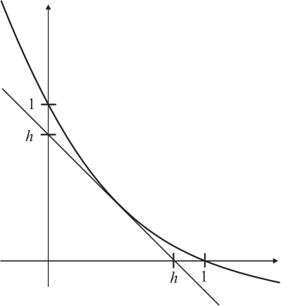
(a) The $\beta$–graph

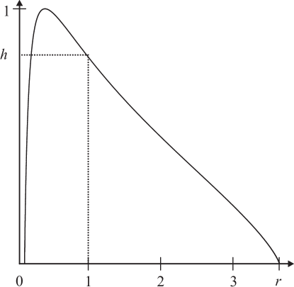
(b) The Lyapunov spectrum $s\mapsto\dim_{H}(\mathcal{L}(s))$.

Figure 2. The $\beta$-graph and the graph of the Lyapunov dimension spectrum in the Salem case for $\tau=0.08$; in both figures $h=0.8107...$ denotes the Hausdorff dimension of $\mathcal{D}_{\sim}$. The conjugacy $\Theta_{\tau}$ is $1/r$-Hölder regular.

Finally, let us mention that one can also explicitly calculate the number $s_{0}(S_{\tau})$ which is determined by $\beta_{\tau}^{\prime}(s_{0}(S_{\tau}))=-1$. A straight forward calculation gives that

$$s_{0}(S_{\tau})=\left(\log(\tau^{-1}-1)\right)^{-1}\log\left(\frac{\log(2\tau)}{\log(2/(1-\tau))}\right).$$

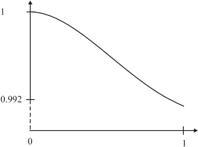
(a) The graph of $\tau\rightarrow\dim D_{\sim}(R_{\tau},T)$ for the sine family with parameter $\tau$ .

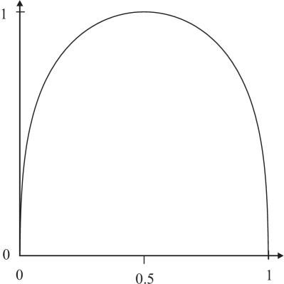
(b) The graph of $\tau\rightarrow\dim D_{\sim}(S_{\tau},T)$ for the Salem family with parameter $\tau$ .

Figure 3. The two dimension spectra.

Example 2 (The Sine Family): Let $T$ be given as in the previous example, and for each $\tau\in(0,1)$ let the map $R_{\tau}:\mathcal{U}\to\mathcal{U}$ be defined by

$$R_{\tau}(\xi):=2\xi+\frac{\tau}{2\pi}\sin(2\pi\xi)\mod 1,\,\mbox{ for each }\,\xi\in\mathcal{U}.$$

The associated conjugacies $\Psi_{\tau}$ are then given by $\Psi_{\tau}\circ R_{\tau}=T\circ\Psi_{\tau}$ (see Fig. 4). We can then use Theorem 1.1 to compute the Hausdorff dimension of the set $\mathcal{D}_{\sim}(R_{\tau},T)$ of points at which $\Psi_{\tau}$ is not differentiable in the generalised sense. This is plotted as a graph in Fig 3. (Note that taking the conjugacy in the other direction would yield exactly the same result).

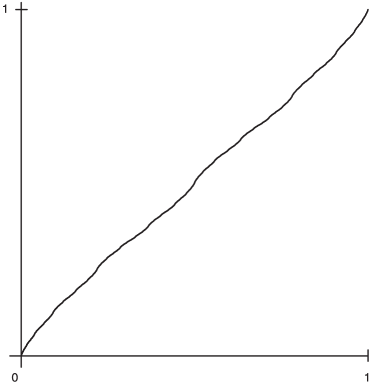
(a) $\tau=0.4$

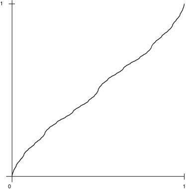
(b) $\tau=0.8$

Figure 4. The graphs of the conjugating maps $\Psi_{\tau}$ for $\tau=0.4$ and $\tau=0.8$ in the sine-family example.

5. Proofs of Propositions 1.4 and 1.5

Proof of Proposition 1.4: We start by observing that the Hausdorff dimension of the set $\mathcal{D}_{\sim}$ depends regularly on the expanding maps. Let $T_{\tau}:\mathcal{U}\to\mathcal{U}$ be elements of the Banach manifold of the $C^{k}$-family of expanding maps, with a $C^{k}$ dependence on $\tau\in(-\epsilon,\epsilon)$, say, and assume that $T_{0}$ is the usual $d$-to-$1$ linear expanding map. Let $0=a_{0}^{(\tau)}<a_{1}^{(\tau)}<\cdots a_{d-1}^{(\tau)}<a_{d}^{(\tau)}=1$ denote the $T_{\tau}$-preimages of zero. For each $\alpha>0$, we then define the operator $\mathcal{T}_{\tau}:C^{\alpha}(\mathcal{U},{\mathbb{R}})\to C^{\alpha}(\mathcal{U},{\mathbb{R}})$ on the space of $\alpha$-Hölder continuous functions (see e.g. [7]) by

$$(\mathcal{T}_{\tau}h)(\xi):=\frac{1}{d}h\left(\{T_{\tau}(\xi)\}\right)+\frac{j}{d},\,\text{ for each }\xi\in[a_{j}^{(\tau)},a_{j+1}^{(\tau)}],j\in\{0,...,d-1\}.$$

Also, with $\|h\|_{\infty}$ denoting the usual supremum norm, we define a norm $\|\cdot\|$ on $C^{\alpha}(\mathcal{U},{\mathbb{R}})$ by

$$\|h\|:=\sup_{\xi\neq\eta}\frac{|h(\xi)-h(\eta)|}{|\xi-\eta|^{\alpha}}+\|h\|_{\infty}.$$

We observe that on each of the intervals $[a_{j}^{(\tau)},a_{j+1}^{(\tau)}]$ we have that

$$|\mathcal{T}_{\tau}h_{1}(\xi)-\mathcal{T}_{\tau}h_{2}(\xi)| \leq \frac{1}{d}|h_{1}(T_{\tau}(\xi))-h_{2}(T_{\tau}(\xi))|$$

$$\leq \frac{1}{d}\|h_{1}-h_{2}\|_{\infty}$$

and

$$|\mathcal{T}_{\tau}(h_{1}-h_{2})(\xi) - \mathcal{T}_{\tau}(h_{1}-h_{2})(\eta)|$$

$$\leq \frac{1}{d}\|h_{1}-h_{2}\|_{C^{\alpha}}|T_{\tau}(\xi)-T_{\tau}(\eta)|^{\alpha}$$

$$\leq \frac{1}{d}\|h_{1}-h_{2}\|_{C^{\alpha}}|T_{\tau}(\xi)-T_{\tau}(\eta)|^{\alpha}$$

$$\leq \left(\frac{1}{d}\|h_{1}-h_{2}\|_{C^{\alpha}}\,\|T_{\tau}\|_{C^{1}}^{\alpha}\right)|\xi-\eta|^{\alpha}.$$

In particular, for $\alpha>0$ sufficiently small we have that $\mathcal{T}_{\tau}$ is a contraction with respect to $\|\cdot\|$. Moreover, $(I-\mathcal{T}_{\tau}):C^{\alpha}(\mathcal{U},{\mathbb{R}})\to C^{\alpha}(\mathcal{U},{\mathbb{R}})$ is invertible, and by the Implicit Function Theorem there exists a $C^{k}$ family $\left\{h_{\tau}\in C^{\alpha}(\mathcal{U},\mathcal{U}):\tau\in(-\epsilon,\epsilon)\right\}$ such that $h_{0}$ is the identity map and $\mathcal{T}_{\tau}h_{\tau}=h_{\tau}$.

Let us consider the map $H_{\tau}:(-\epsilon,\epsilon)\to C^{k-1}(\mathcal{U})\times C^{\alpha}(\mathcal{U})$ given by $H_{\tau}(\tau):=(\log|T_{\tau}^{\prime}|,h_{\tau})$. Clearly, this map is $C^{k-1}$ as a map on Banach spaces. Also, we define the composition operator $\mathcal{O}:C^{k-1}(\mathcal{U})\times C^{\alpha}(\mathcal{U})\to C^{\alpha}(\mathcal{U})$ by $\mathcal{O}(f,g):=f\circ g$, which is $C^{k-2}$, by a result of [4] . We then consider the image of $H_{\tau}$ under $\mathcal{O}$, that is

$$\mathcal{O}\circ H_{\tau}:\tau\mapsto(\log|T_{\tau}^{\prime}|,h_{\tau})\mapsto\mathcal{O}(\log|T_{\tau}^{\prime}|,h_{\tau})=\log|T_{\tau}^{\prime}|\circ h_{\tau}\in C^{\alpha},$$

which is again $C^{k-2}$ [4]. (Note that if instead we would consider $\widetilde{\mathcal{O}}:C^{k-1}(\mathcal{U})\times C^{0}(\mathcal{U})\to C^{0}(\mathcal{U})$, then $\widetilde{\mathcal{O}}(H_{\tau})$ would be $C^{k-1}$; but we need to work with Hölder functions, which causes the loss of an extra derivative.)
Now consider the potential function $\varphi_{\tau}$, given by $\varphi_{\tau}(\xi):=-\log|T_{\tau}^{\prime}(h_{\tau}(\pi_{T_{\tau}}(\xi)))|$ for $\xi\in\mathcal{U}$, and then let $\beta_{\tau}(s)$ be defined implicitly by

$$P(-s\log|T^{\prime}_{\tau}|+\beta_{\tau}(s)\log|T^{\prime}_{0}|)=0.$$

Since the pressure function is analytic, the Implicit Function Theorem implies that the function given by $\tau\mapsto\beta_{\tau}$ is analytic. Also, it follows that the function given by $\tau\mapsto\dim_{H}(\mathcal{D}_{\sim}(T_{\tau},T_{0}))$ is a $C^{k-2}$ function (for an example see Fig. 3). This completes the proof of Proposition 1.4

Proof of Proposition 1.5: The aim is to show that there exists a conjugacy between two elements of the space $C^{2}({\mathbb{S}}^{1})$ of $C^{2}$ expanding circle maps such that the Hausdorff dimension of the set of points at which this conjugacy is non differentiability in the generalised sense is arbitrarily close to $0$. We start by considering the Salem case but where the maps are defined on the circle $\mathbb{S}^{1}$. For ease of exposition, we use the same notation and let $T:\mathbb{S}^{1}\rightarrow\mathbb{S}^{1}$ and $S_{\tau}:\mathbb{S}^{1}\rightarrow\mathbb{S}^{1}$ refer to the circle maps which correspond to the interval maps defined in Example 1. The corresponding conjugacy $\Theta_{\tau}$ is given as before by $T\circ\Theta_{\tau}=\Theta_{\tau}\circ S_{\tau}$. From our analysis in Example 1 it is clear that $\dim_{H}(\mathcal{D}_{\sim}(S_{\tau},T))$ tends to zero for $\tau$ tending to zero (see Fig. 2). However, whereas $T$ is a $C^{2}$ map of the circle, $S_{\tau}$ is clearly not (although, it is always piecewise expanding $C^{2}$ when viewed as a map of $\mathcal{U}$ into itself). So, in order to find a $C^{2}$ example, we have to apply some suitable perturbations to $S_{\tau}$. For this, let $\beta_{\tau}$ and $\psi,\varphi_{\tau}:\Sigma\rightarrow{\mathbb{R}}$ be given as in Example 1. As before we choose $s_{0}(S_{\tau})$ satisfying $\beta_{\tau}^{\prime}(s_{0}(S_{\tau}))=-1$. For the remaining part of the proof, let $\tau\in(0,1)\setminus\{\frac{1}{2}\}$ be fixed.

$C^{2}$ denseness: We use the metric $d_{\mathrm{KL}}$ considered by Keller and Liverani in [9]. This metric is given, for expanding piecewise $C^{2}$ maps $F$ and $G$ of the unit interval $\mathcal{U}$ into itself, by

$$d_{\mathrm{KL}}(F,G) := \inf\{\gamma>0|\exists X\subseteq\mathcal{U}\text{ }\exists\,\text{ a diffeomorphism }H:\mathcal{U}\rightarrow\mathcal{U}\text{ such that }$$

$$\;\;\;\;\;\;\lambda(X)>1-\gamma,G\left|{}_{X}=F\circ H\right|_{X}\text{ and }$$

$$\;\;\;\;\;\;\forall\xi\in\mathcal{U}:\text{ }|H(\xi)-\xi|<\gamma,\text{ }|1-(H^{-1})^{\prime}(H(\xi))|<\gamma\}.$$

One immediately verifies that there exists a sequence $\left(S^{(n)}\right)_{n\in{\mathbb{N}}}$ of functions in $C^{2}({\mathbb{S}}^{1})$ such that $\lim_{n\rightarrow\infty}d_{\mathrm{KL}}(S^{(n)},S_{\tau})=0$, where the $S^{(n)}$ are viewed as interval maps.

Norms and operators: Let $B_{0}(\mathcal{U}):=\{f:\mathcal{U}\rightarrow{\mathbb{R}}:\|f\|_{0}<\infty\}$ be the Banach space with the combined norm $\|\,\cdot\,\|_{0}$ given by $\|f\|_{0}:=\|f\|_{1}+\|f\|_{BV}$, where $\|\,\cdot\,\|_{1}$ denotes the $L^{1}$ norm and $\|\,\cdot\,\|_{BV}$ the bounded variation seminorm, given by $\sup\{\sum_{i=1}^{n}|f(\xi_{i+1})-f(\xi_{i})|:0\leq x_{1}<\cdots<x_{n}\leq 1,n\in{\mathbb{N}}\}$. Also, let the weak operator norm $\|\,\cdot\,\|_{W}$ be given by $\|\mathcal{L}\|_{W}:=\sup\{\|\mathcal{L}(g)\|_{1}:g\in B_{0}(\mathcal{U}),\text{ }\|g\|_{BV}\leq 1\}$. Finally, for an expanding map $S:\mathcal{U}\rightarrow\mathcal{U}$ we define the transfer operator $\mathcal{L}_{S}:B_{0}(\mathcal{U})\to B_{0}(\mathcal{U})$, for $g\in B_{0}(\mathcal{U})$ and $\xi\in\mathcal{U}$, by

$$\mathcal{L}_{S}g(\xi)=\sum_{S(\eta)=\xi}|S^{\prime}(\eta)|^{-1}g(\eta).$$

Continuity: Firstly, note that it can be shown that $\lim_{n\rightarrow\infty}||\mathcal{L}_{S^{(n)}}-\mathcal{L}_{S_{\tau}}||_{W}=0$ (see comment (a) on page 143 of [9]). Furthermore, by [9, Corollary 1], we have that for each $t\in{\mathbb{R}}$ fixed, that the leading eigenvalues of the operators $\mathcal{L}_{S^{(n)}}$ converge to the leading eigenvalue of $\mathcal{L}_{S_{\tau}}$. That is,

$$\lim_{n\rightarrow\infty}P(t\log|(S^{(n)})^{\prime}|)=P(t\log|S_{\tau}^{\prime}|).$$

Local uniform convergence: Recall that the map given by

$$t\mapsto\beta_{S^{(n)}}(t):=P(-t\log(S^{(n)})^{\prime})/\log 2$$

is differentiable and convex. Using the above ‘Continuity’, we then have that $\lim_{n\to\infty}\beta_{S^{(n)}}(t)=\beta_{S_{\tau}}(t)$, for each $t\in{\mathbb{R}}$ fixed. Since pointwise convergence of sequences of differentiable convex functions implies local uniform convergence (see [17, Theorem 10.8]), we now conclude that

$$\lim_{n\to\infty}\beta_{S^{(n)}}(s_{0}(S^{(n)}))+s_{0}(S^{(n)})=\beta_{S_{\tau}}(s_{0}(S_{\tau}))+s_{0}(S_{\tau}).$$

Since $\beta_{S}(s_{0}(S))+s_{0}(S)=\dim_{H}(\mathcal{D}_{\sim}(S,T))$, this finishes the proof of the proposition.

References

- [1] R. Bowen. Hausdorff dimension of quasi-circles. Publ. Mathématiques IHES, 50 (1979) 11–25.
- [2] R. Darst. The Hausdorff dimension of the non–differentiability set of the Cantor function is . Proc. Amer. Math. Soc. 119 (1993) 105–108.
- [3] G. Cui. On the smoothness of conjugacy for circle covering maps. Acta Math. Sinica (N.S.) 12 , no. 2 (1996) 122–125.
- [4] R. de la Llave and R. Obaya. Regularity of the composition operator in spaces of Hölder functions. Discrete Contin. Dynam. Systems 5 (1999), no. 1, 157–184.
- [5] M. Denker, W. Philipp. Approximation by Brownian motion for Gibbs measures and flows under a function, Ergodic Theory and Dynamical Systems 4 (1984) 541–552.
- [6] K.J. Falconer. One-sided multifractal analysis and points of non-differentiability of devil’s staircases. Math. Proc. Camb. Phil. Soc. 136 (2004) 67–174.
- [7] B. Hasselblatt and A. Katok. Introduction to the modern theory of dynamical systems. With a supplementary chapter by Katok and Leonardo Mendoza. Encyclopedia of Mathematics and its Applications, 54. Cambridge University Press, Cambridge, 1995
- [8] Y. Jiang. Renormalization and geometry in one-dimensional and complex dynamics, Advanced Series in Nonlinear Dynamics 10, World Sci. Publ., 1996.
- [9] G. Keller and C. Liverani. Stability of the spectrum for transfer operators. Ann. Scuola Norm. Sup. Pisa Cl. Sci. (4) 28 (1999), no. 1, 141–152
- [10] M. Kesseböhmer, B.O. Stratmann, Hölder-differentiability of Gibbs distribution functions. Oberwolfach preprints 13 (2007).
- [11] M. Kesseböhmer, B.O. Stratmann, Fractal analysis for sets of non-differentiability of Minkowski’s question mark function. To appear in J. Number Theory (2008).
- [12] M. Kesseböhmer, B.O. Stratmann. A multifractal analysis for Stern-Brocot intervals, continued fractions and Diophantine growth rates. J. reine angew. Math. 605 (2007) 133–163.
- [13] A. Manning, A relation between Lyapunov exponents, Hausdorff dimension and entropy. Ergodic Theory and Dynamical Systems 1 (1981), no. 4 (1982) 451–459.
- [14] H. Minkowski. Verhandlungen des III. internationalen Mathematiker-Kongresses in Heidelberg, 1904. Also to be found in Gesammelte Abhandlungen, 1991, Vol. 2 (1991) 50–51.
- [15] G.D. Mostow. Strong rigidity of locally symmetric spaces. Annal. Math. Studies 78, Princeton Univ. Press, 1972.
- [16] Ya. B. Pesin. Dimension theory in dynamical systems. Contemporary views and applications. Chicago Lectures in Mathematics. University of Chicago Press, Chicago, IL, 1997.
- [17] R. T. Rockafellar. Convex analysis. Princeton Math. Ser. 28, Princeton N. J., 1970.
- [18] R. Salem. On some singular monotonic functions which are strictly increasing. Trans. Amer. Math. Soc., 53 (1943) 427–439.
- [19] M. Shub, D. Sullivan. Expanding endomorphisms of the circle revisited. Ergodic Theory and Dynamical Systems 5 (1985) 285–289.
- [20] D. Sullivan. Quasiconformal homeomorphisms in dynamics, topology, and geometry. Proceedings of the International Congress of Mathematicians, Vol. 1, 2 (Berkeley, Calif., 1986), 1216–1228, Amer. Math. Soc., Providence, RI, 1987.
- [21] Lai-Sang Young, Dimension, entropy and Lyapunov exponents. Ergodic Theory and Dynamical Systems 2 , no. 1 (1982) 109–124.