Dependence of the liquid-vapor surface tension on the range of interaction: a test of the law of corresponding states

Abstract

The planar surface tension of coexisting liquid and vapor phases of a fluid of Lennard-Jones atoms is studied as a function of the range of the potential using both Monte Carlo simulations and Density Functional Theory. The interaction range is varied from $r_{c}^{*}=2.5$ to $r_{c}^{*}=6$ and the surface tension is determined for temperatures ranging from $T^{*}=0.7$ up to the critical temperature in each case. The results are shown to be consistent with previous studies. The simulation data are well-described by Guggenheim’s law of corresponding states but the agreement of the theoretical results depends on the quality of the bulk equation of state.

I Introduction

One of the most fundamental properties of a fluid is the surface tension at the liquid-vapor interface. It would seem that such a fundamental property would be an ideal candidate for study via computer simulation. However, the determination of the surface tension from simulation turns out to be frought with difficulties so that even today there is still a substantial amount of effort directed towards the development of more reliable algorithms and the refinement of the reported values even for the paradigmatic case of a simple fluid modeled with the Lennard-Jones interactionMecke et al. (1997). One of the primary difficulties is that in all simulations, the potential is truncated at some finite range and it happens that the surface tension is very sensitive to the value of the cutoff. For that reason, an important part of the development of algorithms has focused on the calculation of the corrections needed to get the infinite-ranged limit from data obtained using a truncated potential (see, e.g., ref. Mecke et al. (1997); Duque and Vega (2004)). This sensitivity is therefore a nuisance when the goal is to get the infinite range result, but in other ways it can made useful. In particular, one of the important reasons to determine the surface tension from simulation is that it provides a baseline against which theories of inhomogeneous liquids can be testedKatsov and Weeks (2002); Lutsko (2008). For this application, the sensitivity of the surface tension to the range of the potential can be used as a test of the generality of a theory which was probably motivated in the first place by its agreement with some existing simulation data. Furthermore, there has recently been a significant increase in interest in short-ranged potentials in their own right. This is due to the fact that certain complex fluids, in particular globular proteins, can, in a first approximation, be modeled as a simple fluid with a very short ranged interactionten Wolde and Frenkel (1997). It is therefore interesting to study the properties of fluids with these kinds of interactions and to test that existing theories work in this new domain of interest. For these reasons, we present in this paper a systematic study of the dependence of the surface tension of a Lennard-Jones fluid as a function of the range of the potential.

In this paper, we describe the results of Monte Carlo (MC) simulations of a Lennard-Jones fluid with the potential truncated at several different points. We have chosen to truncate and shift the Lennard-Jones potential, $v_{LJ}(r)$, so that the potential used in this work is $v(r;r_{c})=v_{LJ}(r)-v_{LJ}(r_{c})$ for $r<r_{c}$ and $v(r)=0$ for $r\geq r_{c}$. If this shift is not performed, then there is an impulsive contribution to the pressure when atoms move across the $r=r_{c}$ boundary that would have to be taken into accountFrenkel and Smit (2001). We do not shift the force, i.e. we do not use $\tilde{v}(r;r_{c})=v_{LJ}(r)-v_{LJ}(r_{c})-(r-r_{c})v_{LJ}^{\prime}(r_{c})$ with $v_{LJ}^{\prime}(r)=dv_{LJ}(r)/dr$ inside the cutoff, as is usually done in molecular dynamics simulations to avoid impulsive forces: our potential is truncated and shifted but the force is not shifted. This choice was made in order to allow for comparison with previous MC studies.

In the simulations a slab of liquid is bounded on both sides by vapor. The surface tension is determined using the method of BennettBennett (1976); Frenkel and Smit (2001) as there seems to be some evidence that this method is more robust than other commonly used techniquesErrington and Kofke (2007). It is often the case that the quantity of interest is the surface tension for the infinite-ranged potential. Since simulations almost always make use of truncated potentials, various techniques have been developed to approximate the so-called long range corrections, i.e. the difference between quantities calculated with the truncated potential and the infinite-ranged quantitiesDuque and Vega (2004). We do not include any such corrections here since our goal is actually to study the truncated potentials. Thus, each value of the cutoff defines a different potential with its own coexistence curve and thermodynamics.

In Section II, we present the simulation techniques used in our work. Section III contains a discussion of our results including a comparison to previous work. Since one of the motivations for this work is to provide a baseline for testing theories of the liquid state, we illustrate this by comparing our results to Density Functional Theory (DFT) calculations and by testing the law of corresponding states. We give our conclusions in the last Section.

II Simulation Methods

Simulations are performed with a standard Metropolis Monte-Carlo algorithm (MC-NVT) for a system of $N=2000$ particles of mass $m$ at temperature $T$ in a volume $V=L_{x}L_{y}L_{z}$ where $L_{x}$, $L_{y}$, and $L_{z}$ are the dimensions of the rectangular simulation cell. Periodic boundary conditions are used in all directions. Particles interact via the Lennard-Jones potential,

$$v_{LJ}(r)=4\epsilon\left(\left(\frac{\sigma}{r}\right)^{12}-\left(\frac{\sigma}{r}\right)^{6}\right)$$ (1)

which is truncated and shifted so that the potential simulated is

$$v(r)\,=\,\left\{\begin{array}[]{r@{\quad:\quad}l}v_{LJ}(r)-\,v_{LJ}(r_{c})&r\,<\,r_{c}\\ 0&r\geq r_{c}\end{array}\right.$$ (2)

where $r_{c}$ is the cutoff radius. Each simulation starts from a rectangular box ($L_{x}=L_{y}=L$, $L_{z}=4\,L$) filled with a dense disordered arrangement of particles ($\rho^{\ast}\equiv\rho\sigma^{3}=0.8$) surrounded along the z-direction by two similar rectangular boxes containing particles in a low density state ($\rho^{\ast}\sim 0.01$) . The total simulation box has sides of length $L_{x}=L_{y}=9.15\sigma$ and $L_{z}=109.63\sigma$. The liquid film located in the middle of the box has a thickness $\Delta z\simeq 27\sigma$ so that the two interfaces do not influence each others. The system is first equilibrated during $5\times 10^{5}$ Monte-Carlo cycles (one cycle $=\,N$ updates) after which the positions of the particles are saved every $20$ cycles during $5\times 10^{5}$ cycles. This ensemble of $2.5\times 10^{4}$ configurations is used to compute the density profile and the surface tension by the Bennett’s method.

Although several methods are available for the computation of the surface tension, the Bennett’s approach has been chosen because of its accuracyErrington and Kofke (2007). In the Bennett’s method the calculation of the surface tension follows from the definition

$$\gamma\,=\,\left(\frac{\partial F}{\partial A}\right)_{N,V,T}$$ (3)

where $F$ is the free energy and $A$ is the area of the liquid-vapor interface. In its implementation the method requires that one performs two simulations: one for system $0$ of interface area $A_{0}$, and another for system $1$ of interface area $A_{1}=A_{0}+\Delta A$. In this work $\Delta A/A=5\times 10^{-4}$. The free energy difference $\Delta F$ between the two systems is evaluated by the method of acceptation ratio which starts with the computation of $\Delta E_{01}=E_{01}-E_{00}$ which is the difference between $E_{00}$, the energy of a configuration of system $0$, and $E_{01}$, the energy of a new configuration obtained from the previous one by rescaling the positions of the particlesSalomons and Mareschal (1991); Frenkel and Smit (2001) : $x^{\prime}=x\,(A_{1}/A_{0})^{\frac{1}{2}}$, $y^{\prime}=y\,(A_{1}/A_{0})^{\frac{1}{2}}$, and $z^{\prime}=z\,(A_{0}/A_{1})$. Similarly one computes $\Delta E_{10}=E_{10}-E_{11}$ obtained from a configuration of system $1$ following an inverse rescaling of the positions. $\Delta F$ is obtained by requiring that

$$\sum_{n_{0}}\,f(\Delta E_{01}-\Delta F)\,=\sum_{n_{1}}\,f(\Delta E_{10}+\Delta F)$$ (4)

where $\sum_{n_{0}}$ ($\sum_{n_{1}}$) is a sum over the configurations of systems $0$ ($1$), and $f(x)=(1+\exp(\beta x))^{-1}$. Then, taking into account the fact that the system contains two flat interfaces, the value of the surface tension is given by $\gamma=\Delta F/(2\Delta A)$ .

III Results

III.1 Comparison to previous results

Our results for the surface tension as a function of the cutoff are given in Table 1. Note that all quantities are reported in reduced units so that the reduced temperature is $T^{\ast}=T/\epsilon$, the reduced cutoffs are $r_{c}^{\ast}=r_{c}/\sigma$ and the reduced surface tension is $\gamma^{\ast}=\gamma\sigma^{2}/\epsilon$. In Fig. 1 we show our results for cutoffs of $r_{c}^{*}=2.5$ and $6.0$ compared to the MC data of Haye and BruinHaye and Bruin (1994) for the shorter cutoff and to the MD data of Duque et alDuque et al. (2004) (who appear to shift the forces) and Potoff et alPotoff and Panagiotopoulos (2000) and Mecke et alMecke et al. (1997). The latter two are shown even though they include long-ranged corrections. Our data are seen to be very consistent with the MC data obtained without long-ranged corrections and to lie slightly below the corrected data, as expected.

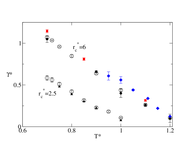
Figure 1: (Color online)The surface tension as a function of temperature for two different cutoffs. The open circles are our data, the filled circles are from Duque et alDuque et al. (2004), the squares are from Mecke et alMecke et al. (1997), the diamonds are from Potoff et alPotoff and Panagiotopoulos (2000) and the triangles are from Haye and Bruin (1994)). Note that the Mecke and Potoff data both include long-ranged corrections.

III.2 Comparison to DFT

In Fig. 2, we compare our results to the predictions of a recently proposed Density Functional Theory modelLutsko (2008). The DFT requires knowledge of the bulk equation of state and the figure shows results using two different inputs: the 33-parameter equation of state of Johnson, Zollweg and Gubbins (JZG)Johnson et al. (1993) and first order Barker-Henderson thermodynamic perturbation theoryBarker and Henderson (1967); Hansen and McDonald (1986). Both versions of the theory are in good qualitative agreement with the data, showing the decrease in surface tension as the range of the potential decreases. It might be thought that use of an empirical equation of state should automatically give superior results to an approximation, like thermodynamic perturbation theory, but this is not necessarily the case since the equation of state is fitted to data for the infinite-ranged potential. The finite cutoff is accounted for using simple mean-field correctionsJohnson et al. (1993); Frenkel and Smit (2001) and these become increasing inaccurate as the cutoff becomes shorter and, for fixed cutoff, as the fluid density becomes higher. The latter condition means, in the present context, increasing inaccuracy as the temperature decreases. Both of these trends are confirmed by the figure. The decrease in accuracy with decreasing cutoff can be seen in the fact that the critical point (corresponding to the temperature at which the surface tension extrapolates to zero) is less accurately estimated for the smaller cutoffs than for the larger cutoffs.

The perturbation theory, on the other hand, takes the cutoff into account more accurately and consistently so that no strong change in accuracy is expected as the cutoff decreases. However, the theory itself is expected to be less accurate for higher densities so again a drop in accuracy with decreasing temperature would be expected and that is indeed seen in the figure. Furthermore, perturbation theory is in general going to be inaccurate near the critical point as it does not take into account renormalization effects which tend to lower the critical point. These effects are less pronounced for shorter-ranged potentials and indeed the perturbation theory seems more consistent with shorter-ranged potential.

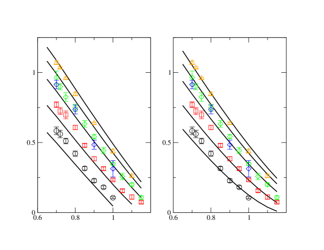
Figure 2: (Color online)Comparison of our simulation data to a DFT modelLutsko (2008). The panel on the left shows the results of the theory using an empirical equation of state while the results on the right were obtained using thermodynamic perturbation theory.The lines are ordered from the smallest cutoff (lowest lines) to the largest cutoff (highest lines) and were calculated for $r_{c}^{*}=2.5,3,4,6,\infty$. The data is represented by circles(2.5), squares(3), diamonds(4), filled diamonds (4 - larger system) and triangles(6).

Table 1: Surface tension determined from simulation as a function of temperature for different cutoffs.

Temperature	$r_{c}^{*}=2.5$	$r_{c}^{*}=3$	$r_{c}^{*}=4$	$r_{c}^{*}=4$	$r_{c}^{*}=6$
0.70	0.584 (27)	0.770 (21)	0.964(46)	0.914(30)	$1.070(13)$
0.72	0.561 (26)	0.726 (25)	0.899(22)		$1.034(7)$
0.75	0.511 (20)	0.698 (28)	0.825(31)		$0.959(8)$
0.80	0.421 (19)	0.608 (16)	0.748(25)	0.736 (32)	$0.847(13)$
0.85	0.315 (13)	0.480 (12)	0.633(24)
0.90	0.228 (13)	0.384 (15)	0.542(16)	0.484(33)	$0.638(8)$
0.95	0.181 (11)	0.314 (12)	0.443(22)
1.0	0.106 (7)	0.234 (8)	0.348(11)	0.313 (59)	$0.438(15)$
1.05		0.156 (11)	0.258(23)
1.1		0.111 (16)	0.200 (12)		$0.261(13)$
1.15		0.074 (10)	0.108 (14)
1.2		0.054 (6)	0.067 (15)	0.063 (19)	$0.105(5)$

III.3 Corresponding states

The principle of corresponding states is a generalization of the results of the van der Waals equation of stateGuggenheim (1945). The idea is that the properties of simple liquids should be universal functions of the state variables, density and temperature, scaled to the critical point. In this section, we test this hypothesis by applying it to the surface tension. The first step is therefore to determine the critical temperatures and densities of the various truncated potentials. Since the theoretical calculations require as input an equation of state, the critical points are easily determined. To determine them from the simulations, we took five independent averages over 5000 configurations and fitted the density profiles in each case to a hyperbolic tangent and then from these extract the coexisting vapor and liquid densities at each temperature. The five values obtained at each temperature were averaged and the variance used as an estimate of the errors in the values. The critical temperature was then estimated by using the lowest order renormalization group (RG) result, $\frac{1}{2}(\rho_{l}-\rho_{v})=A(T_{c}-T)^{0.325}$Le Guillou and Zinn-Justin (1977, 1980). In some applicationsOkumura and Yonezawa (2000), higher order terms are included but we did not feel that the accuracy of our data warranted use of anything but the lowest order function. The critical density was then estimated using the law of the rectilinear diameter, $\frac{1}{2}(\rho_{l}+\rho_{v})=\rho_{c}+B(T_{c}-T)$Guggenheim (1945). There are again higher order corrections to this formula which can be calculated using RG methods, but for the reasons just given, we have not attempted to include them. The results of these fits are illustrated in Fig. 3 and summarized in Table 2. The largest errors in this procedure are in the determination of the critical density.

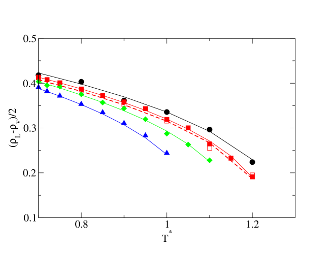
Figure 3: (Color online) The fit of the difference in liquid and vapor densities, as determined from simulation (symbols), to the RG functional form (lines). The data are shown as circles ($R_{c}=6.0$), open squares ($R_{c}=4.0$, larger cell), filled squares ($R_{c}=4.0$, smaller cell), diamonds ($R_{c}=3.0$) and triangles ($R_{c}=2.5$).

Table 2: The critical points for the LJ potential truncated at different values. The theoretical values were determined using the empirical JZG equation of stateJohnson et al. (1993) (JZG) and the first order Barker-Henderson perturbation theory (BH).

$R^{*}_{c}$	MC		Theory - JZG		Theory - BH
	$T^{*}_{c}$	$\rho^{*}_{c}$	$T^{*}_{c}$	$\rho^{*}_{c}$	$T^{*}_{c}$	$\rho^{*}_{c}$
2.5	1.10 (1)	0.31 (9)	1.04	0.26	1.18	0.325
3.0	1.18 (1)	0.31 (7)	1.15	0.28	1.27	0.342
4.0	1.26 (1)	0.31 (5)	1.25	0.32	1.34	0.341
4.0	1.25 (2)	0.30 (6)	—	—	—	—
6.0	1.30 (2)	0.32 (9)	1.29	0.35	1.38	0.341
$\infty$	1.31	0.317	1.311	0.351	1.40	0.312

Figure 4 shows the surface tensions, as determined from simulation and theory using the JZG equation of state, scaled to the critical density and temperature as a function of distance from the critical temperature. Despite the wide range of cutoffs and the mixture of data from simulations and theory, it is nevertheless seen that the data do in fact obey the law of corresponding states to a good approximation. However, the same scaling of the theoretical calculations using the equation of state from thermodynamic perturbation theory, shown in Figure 5, does not give a single curve. While the data for the shorter cutoffs, $r_{c}^{*}=2.5$ and $r_{c}^{*}=3$ appear to coincide, the data for the larger cutoffs does not. This appears to be due, at least in part, to the fact that the estimate of the critical density as a function of the cutoff calculated using the perturbation theory is not monotonic (see Table 2) which is at odds with the quantities as determined from simulation which clearly are monotonic in the cutoff.

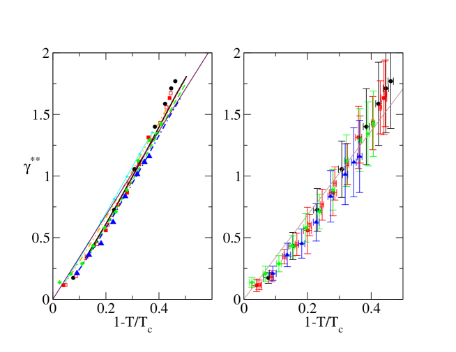
Figure 4: (Color online) The scaled surface tension, $\gamma^{**}\equiv\frac{\gamma}{T_{c}\rho_{c}^{2/3}}$, as a function of distance from the critical temperature. The left panel includes the theoretical curves, shown as full line ($R^{*}_{c}=\infty$), dotted line ($R_{c}^{*}=8$), dashed line ($R_{c}^{*}=6$), dash-dot line ($R_{c}^{*}=4$), dash-dot-dot line ($R_{c}^{*}=3$), and line+circles ($R_{c}^{*}=2.5$), and the simulation data, shown as circles ($R_{c}^{*}=6$), filled squares ($R_{c}^{*}=4$, 2000 atoms), open squares ($R_{c}^{*}=4$, 8000 atoms), diamonds ($R_{c}^{*}=3$) and triangles ($R_{c}^{*}=2.5$). The right hand panel shows only the data from simulation as well as the estimated error. In both cases, the thin line is a best fit to all of the data (theory and simulation) of the form $\gamma^{*}=\gamma^{*}_{0}(1-T/T_{c})$ with $\gamma^{*}_{0}=3.41$.

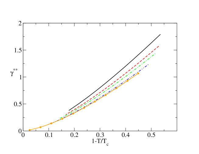
Figure 5: (Color online) The scaled surface tension, $\gamma^{**}\equiv\frac{\gamma}{T_{c}\rho_{c}^{2/3}}$, as a function of distance from the critical temperature as calculated using the perturbative equation of state displayed as a full line ($R^{*}_{c}=\infty$), dashed line ($R_{c}^{*}=6$), dash-dot line ($R_{c}^{*}=4$), dash-dot-dot line ($R_{c}^{*}=3$), and line+circles ($R_{c}^{*}=2.5$).

IV Conclusions

We have presented our determination of the liquid-vapor surface tension in a Lennard-Jones fluid as a function of the range of the potential. The data give a systematic picture of the variation of surface tension with the cutoff and are in agreement with previous studies. It is hoped that this can serve as a useful benchmark for the development of theories of inhomogeneous liquids. Indeed, the results were compared here to calculations made using a recently developed DFT and the strengths and weaknesses of the theory are evident: while it gives a good semi-quantitative estimate of the surface tension for all cutoffs, errors on the order of 10% are present indicating that further improvement is possible.

We have also tested the law of corresponding states by showing our results from both simulation and theory scaled to the critical density and temperature. For the simulation data and the theoretical calculations based on an empirical equation of state, the law of corresponding states appears to be obeyed. However, the calculations based on the equation of state from first order perturbation theory do not appear to scale well at all. This failure appears to be due to poor behavior of the critical density as a function of the cutoff and indicates that care must be exercised before using the law of corresponding states to extrapolate calculations.