A near-infrared interferometric survey of debris disc stars

Abstract

Aims. We aim at directly detecting the presence of optically thin circumstellar dust emission within the terrestrial planetary zone around main sequence stars known to harbour cold debris discs. The present study focuses on a sample of six bright A- and early F-type stars.

Methods. High-precision interferometric observations have been obtained in the near-infrared $K$ band with the FLUOR instrument installed on the CHARA Array. The measured squared visibilities are compared to the expected visibility of the stellar photospheres based on theoretical photospheric models taking into account rotational distortion. We search for potential visibility reduction at short baselines, a direct piece of evidence for resolved circumstellar emission.

Results. Our observations bring to light the presence of resolved circumstellar emission around one of the six target stars ($\zeta$ Aql) at the $5\sigma$ level. The morphology of the emission source cannot be directly constrained because of the sparse spatial frequency sampling of our interferometric data. Using complementary adaptive optics observations and radial velocity measurements, we find that the presence of a low-mass companion is a likely origin for the excess emission. The potential companion is characterised by a $K$-band contrast of four magnitudes. It has a most probable mass of about $0.6M_{\odot}$ and is expected to orbit between about 5.5 AU and 8 AU from its host star assuming a purely circular orbit. Nevertheless, by adjusting a physical debris disc model to the observed Spectral Energy Distribution of the $\zeta$ Aql system, we also show that the presence of hot dust within 10 AU from $\zeta$ Aql, producing a total thermal emission equal to $1.69\pm 0.31$% of the photospheric flux in the $K$ band, is another viable explanation for the observed near-infrared excess. Our re-interpretation of archival near- to far-infrared photometric measurements shows however that cold dust is not present around $\zeta$ Aql at the sensitivity limit of the IRS and MIPS instruments onboard Spitzer, and urges us to remove $\zeta$ Aql from the category of bona fide debris disc stars.

Conclusions. The hot debris disc around Vega (Absil et al. 2006) currently remains our only secure resolved detection within the context of this survey, with six genuine early-type debris disc stars observed so far. Further observations will be needed to assess whether $\zeta$ Aql also belongs to this hot debris disc category.

1 Introduction

Debris discs are optically thin, gas-poor dust discs around main sequence (MS) stars. The presence of circumstellar dust around stars with ages above $\sim$10 Myr is attributed to populations of planetesimals that were neither used to make up planets nor ejected from the system by the time the nebular gas was dispersed (Mann et al. 2006). These leftovers produce dust by mutual collisions and comet-type activity. Being continuously replenished by small bodies, the disc can then persist over much of the star’s lifetime. Due to its large total cross-section area, dust is much easier to observe than planets, not to speak of planetesimals. On the other hand, distributions of dust respond to the presence of planetary perturbers, reflect distributions of the parent bodies and bear important memory of the planetary formation process in the past. Hence debris discs can be used as sensitive tracers of planets, as well as small body populations, and should reflect evolutionary stages of planetary systems. This explains the substantial effort invested in the observation and modelling of debris discs over the last two decades.

Early-type stars, and A-type stars in particular, have been the most successfully studied targets in the context of debris disc studies so far. This is due to a great extent to their intrinsic brightness, which efficiently lights up their debris discs up to large distances (Earth-like temperatures occur at about 5 AU from such stars). Additionally, their MS lifetimes ($\sim$800 Myr) are long enough to encompass the main evolutionary stages of a typical planetary system. Far-infrared surveys carried out with space satellites have been particularly successful in detecting cold dust around nearby A-type stars. For instance, Spiter/MIPS observations of 160 A-type MS stars have shown that about 33% of such stars possess significant excess emission at 24 and 70 $\mu$m (Su et al. 2006), which represents a considerably higher excess rate than what has been found for old solar analogs and M dwarfs (Bryden et al. 2006).

Unlike these successful detections of cold debris in the far-infrared, the discovery of warm ($\sim$300 K) or hot ($\sim$1000 K) dust through mid- and near-infrared observations has been limited to a very small number of targets so far. Furthermore, the rare detections have generally been obtained for young MS stars showing strong mid-infrared silicate features, such as $\beta$ Pic ($\sim$12 Myr, Pantin et al. 1997), HD 145263 ($\sim$8 Myr, Honda et al. 2004), $\eta$ Tel ($\sim$12 Myr, Chen et al. 2006) or HD 172555 ($\sim$12 Myr, Chen et al. 2006). At such ages, planetary systems are still expected to be in the process of forming planets, especially in the inner part of the disc ($<10$ AU) where rocky planets may take up to one hundred Myr to accrete most of the small bodies on nearby orbits and reach their final mass (see Kenyon & Bromley 2006, for a solar-mass star). The observed large mid-infrared excesses are therefore expected to be related to the end of the planet building phase rather than to the dust produced by the collisional grinding of an evolved planetary system, similar to the zodiacal dust in our solar system. For “mature” A-type stars, the lack of near- to mid-infrared excess has generally been associated with a dearth of warm dust grains, a suggestion generally confirmed by the presence of inner holes in resolved images around famous objects such as $\alpha$ PsA (Kalas et al. 2005) or $\alpha$ Lyr (Su et al. 2005).

Incidentally, the inner part of debris discs is a very interesting region to study, as it directly probes the location where planets are supposed to have formed and evolved—conversely, the outer part of the disc ($>20$ AU), similarly to the Kuiper belt in our solar system, only bears a memory of the outermost massive planets through gravitational interactions such as mean motion resonances (see e.g. Reche et al. 2008). The characterisation of inner debris discs is therefore crucial for an understanding of the formation, evolution and dynamics of planetary systems (including our own solar system), as well as to set the scene for the emergence of life on rocky planets.

Reaching a better sensitivity to the inner part of debris discs has thus been an important challenge during the past years, and the detection of small amounts of hot dust around mature early-type stars has finally been enabled by the advent of high-precision near-infrared stellar interferometry. Using the VLTI/VINCI instrument, Di Folco et al. (2004) derived upper limits to the $K$-band dust emission around five stars. The first robust resolved detection of hot dust was obtained for the bright A0V-type star $\alpha$ Lyr (Vega) by Absil et al. (2006) with CHARA/FLUOR on an optimised set of interferometric baselines, showing the presence of extended emission accounting for $1.29\pm 0.19$% of the photospheric flux in the $K$ band. This result was already suggested by Ciardi et al. (2001), although with a large uncertainty on the flux ratio.

This recent detection has raised a number of questions regarding the nature and origin of inner dust grains. In particular, a scenario involving the presence of star-grazing comets, injected into the inner planetary system by dynamical perturbations caused by migrating planets, has been proposed, inspired by the Late Heavy Bombardment (LHB) that happened in the early solar system (Gomes et al. 2005). A similar scenario is also proposed by Wyatt et al. (2007) to explain the presence of warm dust ($\sim$300 K) detected by the Spitzer Space Telescope around a few solar-type stars. We have thus decided to initiate a near-infrared interferometric survey of nearby debris disc stars to assess the occurrence of hot excesses around MS stars. The first paper of this series (Di Folco et al. 2007, hereafter Paper I) focused on two solar-type stars, showing the presence of hot dust around $\tau$ Cet. In this paper, we discuss early-type stars, which hold a privileged position in our survey because their brightness makes them well suited for an interferometric study.

2 Methodology and stellar sample

The principle of debris disc detection by stellar interferometry is based on the fact that the stellar photosphere and its surrounding dust disc have different spatial scales. For an A-type star at a distance of 20 pc, the angular diameter of the photosphere is typically about 1 mas, while the circumstellar disc extends beyond the sublimation radius of dust grains, typically located around 10 to 20 mas for black body grains sublimating at $T_{\rm sub}\simeq 1500$ K. In the infrared $K$ band, the debris disc is therefore generally fully resolved at short baselines ($10-20$ m), while the photosphere is only resolved at long baselines ($\sim$200 m). One can take advantage of this fact to isolate the contribution of circumstellar dust by performing visibility measurements at short baselines, where the stellar photosphere is almost unresolved. The presence of resolved circumstellar emission then shows up as a deficit of squared visibility with respect to the expected visibility of the bare stellar photosphere, as shown in Paper I:

$${\cal V}^{2}(b)\simeq(1-2\epsilon_{\rm CSE}){\cal V}_{\ast}^{2}(b)\,,$$ (1)

where ${\cal V}^{2}$ and ${\cal V}_{\ast}^{2}$ are respectively the squared visibility of the star-disc system and of the bare stellar photosphere, $b$ is the interferometer baseline length, and $\epsilon_{\rm CSE}$ is the flux ratio between the integrated circumstellar emission within the field-of-view and the stellar photospheric emission. This equation is valid only for short baselines and for $\epsilon_{\rm CSE}\ll 1$, as expected for an optically and geometrically thin circumstellar disc.

Due to the expected faintness of the circumstellar emission ($\epsilon_{\rm CSE}\lesssim 1$%), detection needs both a high accuracy on the measured ${\cal V}^{2}$ and on the estimation of the squared visibility ${\cal V}_{\ast}^{2}$ of the bare photosphere at short baselines. While the former has already been demonstrated in the framework of single-mode near-infrared interferometers (e.g., Kervella et al. 2003), the latter is ensured to a large extent by the fact that the stellar photosphere is almost unresolved at short baselines, so that we can tolerate a certain level of imprecision on the knowledge of the stellar angular diameter without jeopardising the detection. For instance, a stellar photosphere with an angular diameter of $1.0\pm 0.1$ mas produces a squared visibility of $0.995\pm 0.001$ at a baseline of 20 m in the $K$ band. Therefore, in the following study, diameter measurements at long interferometric baselines are not required to derive accurate photospheric models, and empirical surface-brightness relations (Kervella et al. 2004) can instead be used to predict stellar angular diameters with a sufficient accuracy, taking into account rotational distortion.

To start our survey of early-type debris disc stars, we have chosen six bright ($K<4$) nearby ($\sim$20 pc) dwarfs, with spectral types ranging from A0 V to F2 V. The main characteristics of our six target stars are summarised in Table 1, together with the already-discussed $\alpha$ Lyr (Absil et al. 2006). All of them have been classified as debris disc stars based on the measurement of a mid- or far-infrared excess emission above the expected photospheric level, using infrared satellites such as IRAS, ISO or the Spitzer Space Telescope.

3 Observations and data reduction

Interferometric observations were obtained in the infrared $K$ band ($1.94-2.34$ $\mu$m) with FLUOR, the Fiber Linked Unit for Optical Recombination (Coudé du Foresto et al. 2003), using the shortest baseline of the CHARA Array formed by the S1 and S2 telescopes (34 metres long, ten Brummelaar et al. 2005). Observations took place during Spring 2006, between April 30th and May 11th.

Table 1: Fundamental parameters and estimated angular diameters for the seven selected targets (including $\alpha$ Lyr). A mean limb-darkened diameter is first computed using Eq. 2—this actually represents the geometric mean of the minor and major axes of the elliptical photosphere. The apparent photospheric oblateness is then estimated by means of Eq. 5, from which we finally deduce the angular diameters for the apparent minor and major axes of the photosphere. The 1$\sigma$ errors are given in superscript.

Name	HD	Type	Dist.	Mass	$v\sin i$	$m_{V}$	$m_{K}$	Mean $\theta_{\rm LD}$	Appar.	Minor $\theta_{\rm LD}$	Major $\theta_{\rm LD}$	Refs.
			(pc)	($M_{\odot}$)	(km s-1)			(mas)	oblat.	(mas)	(mas)
$β$~UMa	95418	A1 V	24.3	2.28	46	$2.35^{0.01}$	$2.38^{0.06}$	$1.095^{0.022}$	1.007	$1.091^{0.022}$	$1.099^{0.022}$	1, 4, 6, 7
$η$~Crv	109085	F2 V	18.2	1.44	92	$4.30^{0.01}$	$3.54^{0.05}$	$0.736^{0.015}$	1.022	$0.728^{0.015}$	$0.744^{0.015}$	1, 4, 6, 8
$σ$~Boo	128167	F2 V	15.5	1.28	15	$4.47^{0.01}$	$3.49^{0.02}$	$0.783^{0.016}$	1.001	$0.783^{0.016}$	$0.783^{0.016}$	1, 4, 6, 9
$α$~CrB	139006	A0 V	22.9	2.58	138	$2.23^{0.01}$	$2.20^{0.05}$	$1.202^{0.024}$	1.059	$1.168^{0.024}$	$1.237^{0.024}$	2, 4, 6, 10
$γ$~Oph	161868	A0 V	29.1	2.18	210	$3.75^{0.01}$	$3.67^{0.05}$	$0.616^{0.012}$	1.107	$0.585^{0.012}$	$0.648^{0.012}$	1, 4, 6, 11
$α$~Lyr	172167	A0 V	7.8	2.30	22	$0.03^{0.01}$	$0.00^{0.02}$	$3.312^{0.067}$	1.002	$3.309^{0.067}$	$3.315^{0.067}$	3, 5, 6, 12
$ζ$~Aql	177724	A0 V	25.5	2.37	317	$2.99^{0.01}$	$2.90^{0.02}$	$0.880^{0.018}$	1.307	$0.770^{0.018}$	$1.006^{0.018}$	1, 4, 6, 13

References.—Masses from (1) Allende Prieto & Lambert 1999, (2) Tomkin & Popper 1986, (3) Aufdenberg et al. 2006; $v\sin i$ from (4) Royer et al. 2002, (5) Hill et al. 2004; $V$ magnitudes from (6) Perryman et al. 1997; $K$ magnitudes from (7) Neugebauer & Leighton 1997, (8) Sylvester et al. 1996, (9) Blackwell et al. 1979, (10) Sneden et al. 1978, (11) Selby et al. 1988, (12) Aumann & Probst 1991, (13) Leggett et al. 1986.

The FLUOR field-of-view, limited by the use of single-mode fibres, has a Gaussian shape resulting from the overlap integral of the incoming turbulent wave fronts with the fundamental mode of the fiber (Guyon 2002). Its actual size depends on the atmospheric turbulence conditions. The estimation of the mean Fried parameter $\langle r_{0}\rangle$ provided by the CHARA array during our observations (7 cm in the visible) allows us to derive a mean value of $0\aas@@fstack{\prime\prime}8$ for the full width at half maximum of the field-of-view. This parameter is sensitive to the actual atmospheric conditions for each individual target star (it typically ranges between $0\aas@@fstack{\prime\prime}7$ and $1\aas@@fstack{\prime\prime}2$), but the only associated effect is to widen the search region for circumstellar emission.

The FLUOR Data Reduction Software (DRS, Coudé du Foresto et al. 1997; Kervella et al. 2004; Mérand et al. 2006) was used to extract the raw squared modulus of the coherence factor between the two independent apertures. The extraction of the squared visibilities from the fringe packets recorded in the time domain is based on the integration of the squared fringe peak obtained by a Fourier transform of the fringe packet (Coudé du Foresto et al. 1997), or equivalently by a wavelet analysis (Kervella et al. 2004). The interferometric transfer function of the instrument was estimated by observing calibrator stars before and after each observation of a scientific target. All calibrator stars (listed in Table 2) were chosen from two catalogues developed for this specific purpose (Bordé et al. 2002; Mérand et al. 2005). Calibrators chosen in this study are late G or K giants, whereas our target stars have spectral types between A0 and F2. Since the visibility estimator implemented in the FLUOR DRS depends on the actual spectrum of the target star, an appropriate correction must be applied to our data, otherwise our squared visibilities would be biased at a level of about 0.3% (Coudé du Foresto et al. 1997). This correction can be based either on the shape factors discussed by Coudé du Foresto et al. (1997) or on a wide band model for estimating the calibrator’s visibilities and interpreting the data (see e.g. Kervella et al. 2003; Aufdenberg et al. 2006). The latter method was chosen for this work, and all the calculations presented here therefore take into account a full model of the FLUOR instrument, including the spectral bandwidth effects.

Table 2: Calibrators chosen from the catalogues of Bordé et al. (2002) and Mérand et al. (2005), listed with spectral type, $K$ magnitude, uniform disc (UD) angular diameter in $K$ band with $1\sigma$ error bar, and associated scientific target(s).

Identifier	Sp. type	$m_{K}$	$\theta_{\rm UD}$ (mas)	Targets
46 Boo	K2 III	2.66	$1.433\pm 0.019$	$\alpha$ CrB
9 CrB	G9 III	3.07	$1.101\pm 0.014$	$\alpha$ CrB
QY Ser	K8 IIIb	1.53	$2.680\pm 0.029$	$\alpha$ CrB
HD 92095	K3 III	2.20	$1.527\pm 0.020$	$\beta$ UMa
HD~100615	K0 III	3.19	$1.027\pm 0.014$	$\beta$ UMa
44 UMa	K3 III	2.04	$1.990\pm 0.023$	$\beta$ UMa
$χ$~Vir	K2 III	2.02	$1.960\pm 0.023$	$\eta$ Crv
HD 108522	K4 III	3.46	$1.171\pm 0.016$	$\eta$ Crv
HD 111500	K4 III	3.05	$1.395\pm 0.020$	$\eta$ Crv
HD 157617	K1 III	2.71	$1.305\pm 0.018$	$\gamma$ Oph
71 Oph	G8 III	2.43	$1.500\pm 0.020$	$\gamma$ Oph,
				$\sigma$ Boo, $\zeta$ Aql
HD 162113	K0 III	3.62	$0.904\pm 0.012$	$\gamma$ Oph
HD 162468	K1 III-IV	3.17	$1.123\pm 0.015$	$\gamma$ Oph
HD 133392	G8 III	3.26	$1.052\pm 0.014$	$\sigma$ Boo
HD 132304	K3 III	3.48	$1.042\pm 0.014$	$\sigma$ Boo
HD 126597	K2 III	3.46	$1.004\pm 0.014$	$\sigma$ Boo, $\gamma$ Oph
HD 176527	K2 III	2.04	$1.721\pm 0.024$	$\zeta$ Aql
HD 175743	K1 III	3.35	$1.106\pm 0.015$	$\zeta$ Aql
$ξ$~Aql	G9.5 IIIb	2.37	$1.620\pm 0.021$	$\zeta$ Aql
$μ$~Aql	K3 IIIb	1.76	$2.240\pm 0.023$	$\zeta$ Aql

4 Estimating stellar angular diameters

A reliable estimation of the photospheric angular diameter is an important pre-requisite for the detection of circumstellar emission at short baselines. In this section, we use surface-brightness relations to estimate the mean photospheric diameter of our target stars. We then apply a standard model of a rotating photosphere in hydrostatic equilibrium to estimate the rotation-induced distortion. Our approach is finally validated by comparison with long-baseline interferometric measurements where available.

4.1 Diameter estimation from surface-brightness relations

Accurate angular diameter estimations for MS stars can be obtained by applying empiric surface-brightness relations (see e.g., Kervella et al. 2004; Di Benedetto 2005), using as input the measured magnitudes in two standard photometric bands. These relations have been calibrated by interferometric measurements (Kervella et al. 2004), and are valid for spectral types from A0 to M2. The smallest intrinsic dispersion ($\sigma\leq 1$%) is obtained by combining $K$- or $L$-band magnitudes with visible magnitudes ($B$ or $V$). Here, we choose to use the $K$-band magnitudes, which are generally known with good accuracy, and combine them with the $V$-band magnitudes measured by Hipparcos (Perryman et al. 1997). $K$ magnitudes have been preferred to $L$ magnitudes, because the potential presence of hot dust around the target stars is expected to affect the $K$ band at a smaller level than the $L$ band—the contrast between a $\sim$9000 K photosphere and $\sim$1000 K surrounding dust decreases with increasing wavelength. In practice, we do not expect the $K$-band magnitudes to be affected by dust emission by an amount larger than 5%, as for higher contributions the signature of hot dust would have already been detected. Our interferometric measurements will confirm this assumption a posteriori. The ($V$, $V-K$) relation, where the $V$ magnitude is used to calibrate the reference magnitude, has been chosen in the present study because of its robustness to dust emission and because the accuracy of the $V$ magnitudes (0.01 mag, Perryman et al. 1997) is better than that of the $K$ magnitudes. The final error bar on the estimated limb-darkened angular diameter $\theta_{\rm LD}$ is therefore generally smaller using the ($V$, $V-K$) relation than the ($K$, $V-K$) relation. The mathematical expression of the ($V$, $V-K$) relation is (see Table 4 from Kervella et al. 2004):

$$\log\theta_{\rm LD}(V,V-K)=0.2753(V-K)+0.5175-0.2V\,.$$ (2)

It has a dispersion of 1% and shows no significant non linearity. The angular diameter estimations for our seven targets are given in the ninth column of Table 1 (“Mean $\theta_{\rm LD}$”).

The associated limb darkening coefficients $u_{K}$ can be found in Claret et al. (1995), assuming a linear limb-darkening law $I_{\lambda}(\mu)=1-u_{\lambda}(1-\mu)$ as in Kervella et al. (2004), where $\mu$ is the cosine of the angle between the perpendicular to the surface of the star and the line of sight. The closest tabulated models to the physical properties of the stars were chosen. It must be noted that the rapid rotation of some of our targets may lead to substantial gravity darkening, so that the tabulated limb darkening coefficients could be underestimated. Fortunately, considering a photosphere 1.0 mas in diameter observed with a 30 m baseline, even a threefold increase of the limb darkening coefficient would produce a variation smaller than 0.1% on the squared visibility (see Eq. 6 in Sect. 5). The case of $\alpha$ Lyr, which is slightly resolved on a 30-m baseline, must however be considered with additional care (see Sect. 4.3).

Estimating the angular diameter of $\alpha$ CrB is a little more complicated than for the other six targets, as it is actually a binary system of Algol type. The primary and secondary are estimated to be A0 V and G5 V stars respectively, and the magnitude difference in $V$ band is estimated to be $\Delta M_{V}=4.89$ (Tomkin & Popper 1986). Based on a $V$-band magnitude of $2.22\pm 0.01$ for the system (Perryman et al. 1997), we adopt a $V$-band magnitude of $2.23\pm 0.01$ for the primary. Then, using the intrinsic colours of MS stars in the infrared (Bessel & Brett 1988), we compute the magnitude difference between the primary and secondary in the $K$ band ($\Delta M_{K}=3.25$), and derive the expected $K$-band photometry of the primary from the system’s photometry in a similar way. The original $K$ magnitude for the binary system, $K=2.14\pm 0.04$ (Sneden et al. 1978), gives a corrected magnitude of $2.20\pm 0.05$, where the error bar has been slightly revised to account for possible errors in the estimation of the spectral types and intrinsic colours of the two components.

4.2 Effect of rapid rotation

With projected rotational velocities up to 317 km s^-1 (Table 1), we expect the photospheres of our target stars to deviate significantly from spherical symmetry due to large centrifugal forces. We will assume in the following study that the apparent photospheric shape can be modelled by an ellipse with semi-major and semi-minor axes noted $R_{a}$ and $R_{b}$, and we force the angular surface of the ellipse to be equal to the angular surface derived from surface-brightness relations in the previous section:

$$R_{a}R_{b}=R_{m}^{2}=\frac{\theta_{\rm LD}^{2}d^{2}}{4}\;,$$ (3)

where $R_{m}$ is the radius of the equivalent spherical photosphere (i.e., the geometric mean of the major and minor radii) and $d$ the distance to the target star. Under the assumptions of hydrostatic equilibrium, uniform rotation, and of a point mass gravitational potential, the apparent rotational velocity $v\sin i$ can be related to the major and minor radii $R_{a}$ and $R_{b}$ with the following equation (Tassoul 1978):

$$v\sin i\simeq\sqrt{2GM\left(\frac{1}{R_{b}}-\frac{1}{R_{a}}\right)}\,.$$ (4)

We define the apparent oblateness ($\rho$) of the photosphere as the ratio of the major and minor radii ($\rho=R_{a}/R_{b}$), and solve the above equation for $\rho$ as a function of $R_{m}$ to obtain:

$$\rho\simeq\left(\frac{(v\sin i)^{2}R_{m}}{4GM}+\sqrt{1+\left(\frac{(v\sin i)^{2}R_{m}}{4GM}\right)^{2}}\right)^{2}\,.$$ (5)

Using the limb-darkened angular radii, masses, and $v\sin i$ listed in Table 1, we derive the apparent oblateness of the photospheres of our seven target stars. They range between 1.001 and 1.307 (see Table 1). From these estimations of oblateness, we can derive the expected angular sizes of the major and minor axes. Since the orientations of the photospheres are unknown, the differences between the major and minor angular radii directly give the additional uncertainty on the stellar diameters along the CHARA S1–S2 baseline due to stellar oblateness. The additional error is typically a few percent of the mean stellar diameter, and reaches 14% for the fastest rotator.

4.3 Long-baseline interferometric measurements

Table 3: Application of surface-brightness relations and of our standard rotating photosphere model to four rapidly rotating stars that have been directly measured with infrared stellar interferometers. The agreement between our estimated mean limb-darkened stellar diameter (“$\theta_{\rm LD}$ model”) and oblateness (“$\rho$ model”) with the measured stellar parameters is very satisfactory. The largest discrepancy between model and observations is found for $\alpha$ Aql and is less than 3%—it should be noted that the interferometric measurements reported on this particular target by Monnier et al. (2007) and Domiciano de Souza et al. (2005) disagree at the $3\sigma$ level (4% of $\theta_{\rm LD}$).

Name	Type	$v\sin i$	Mass	$\theta_{\rm LD}$	$\theta_{\rm LD}$	$\rho$	$\rho$	Ref.
		(km s-1)	($M_{\odot}$)	model	meas.	model	meas.
$α$~Leo	B7 V	317	3.4	1.47	1.47	1.323	1.320	(1)
$α$~Lyr	A0 V	21.9	2.3	3.31	3.31	1.0015	1.0014	(2,3)
$α$~Cep	A7 IV-V	283	2.0	1.51	1.54	1.296	1.298	(4)
$α$~Aql	A7 V	240	1.8	3.31	3.39	1.170	1.164	(5)

References: (1) McAlister et al. (2005), (2) Aufdenberg et al. (2006), (3) Peterson et al. (2006b), (4) van Belle et al. (2006), (5) Monnier et al. (2007).

Since long-baseline infrared interferometric measurements are generally not available for our target stars, we will try to validate our approach by comparison with interferometric measurements of similar MS stars. For the first step of our modelling approach, i.e., surface-brightness relations, such a validation has already been thoroughly addressed by Kervella et al. (2004). Now, for the second step, i.e., the elliptic photospheric model, we can test the validity of Eq. 5 on four rapidly rotating stars with similar masses to our target stars, whose apparent oblateness has been derived from interferometric measurements (see Table 3). The agreement between the modelled apparent oblateness (“$\rho$ model”) and the observed oblateness (“$\rho$ meas.”) is very good.

To improve the accuracy of our angular diameter estimations, actual long baseline interferometric measurements would however be valuable. In the case of $\alpha$ Lyr, such measurements are available, and have been used to produce a realistic model of the stellar photosphere in the $K$ band (Aufdenberg et al. 2006). Using the $K$-band limb profile of Aufdenberg et al. (2006), we have derived an accurate limb-darkened model for the stellar photosphere, giving the following parameters: angular diameter $\theta_{\rm LD}=3.305\pm 0.010$ mas and linear limb-darkening coefficient $u_{K}=0.361$. The angular diameter is slightly smaller than the physical diameter (3.33 mas) derived by Aufdenberg et al. (2006) because the outermost layers of the stellar atmosphere, from $0.992R_{\ast}$ to $R_{\ast}$ (where the pressure is less than 0.01 dynes/cm²), does not contribute significantly to the flux emission. The angular diameter obtained from surface-brightness relations ($3.312\pm 0.067$ mas, see Table 1) is in good agreement with this measurement, although it must be noted that the associated error bar is 7 times larger than that of the directly measured diameter. Nonetheless, we will see in Sect. 5 that the accuracy on the modelled angular diameters displayed in Table 1 is generally sufficient to allow the detection of circumstellar emission at a level as low as 0.1%. The case of $\alpha$ Lyr must be considered separately, because its 3.305 mas photosphere is partly resolved on a 30 m baseline in $K$ band. The error on the modelled photospheric diameter would then induce a large enough uncertainty on the stellar ${\cal V}^{2}$ (about 0.6%) to compromise the detection of circumstellar emission. Moreover, due to gravity darkening, the actual limb-darkening coefficient is much larger than the tabulated one (0.20 in Claret et al. 1995). Therefore, in the rest of this study, we will use for $\alpha$ Lyr the photospheric model of Aufdenberg et al. (2006) described here above.

Another target in our sample has been observed with long-baseline interferometry, this time in the visible range: $\zeta$ Aql was used as a reference star by Peterson et al. (2006a) to calibrate interferometric observations of Altair with the Navy Prototype Optical Interferometer (NPOI). Using archival NPOI data, the authors derived a preliminary model for the $\zeta$ Aql photosphere, giving a minimum angular diameter of $0.815\pm 0.005$ mas. Even though this value is well within our angular diameter range (see Table 1), it is $2.5\sigma$ from the minimum angular diameter that we derive from our rapidly rotating photospheric model ($0.770\pm 0.018$ mas). This discrepancy could partly be due to the wavelength difference between the observations ($V$ band) and the model ($K$ band).

We also note that $\sigma$ Boo has been observed as a calibrator by Boden et al. (2005) at the Palomar Testbed Interferometer (PTI) and at the NPOI. The authors adopted an angular diameter of $0.77\pm 0.04$ mas based on SED modelling of broadband photometry, a value which is consistent with our estimation. They did not mention any significant deviation from that estimated value based on their measurements.

Finally, the eclipsing binary nature of $\alpha$ CrB provides an additional check of our model: Tomkin & Popper (1986) derive a limb-darkened radius of $3.04\pm 0.03\leavevmode\nobreak\ R_{\odot}$ for the primary, which translates into an angular diameter of $1.235\pm 0.012$ mas. This value is most probably representative of the major axis of the photosphere as the rotation axis of the primary and the orbital axis of the binary system are expected to be aligned. The agreement with our major angular diameter ($1.237\pm 0.024$ mas) is very good.

5 Searching for circumstellar emission

To assess the presence of circumstellar emission around a target star, we compare the interferometric ${\cal V}^{2}$ measurements with the expected squared visibility of the stellar photosphere, using the oblate photospheric model presented in the previous section. Assuming a linear limb darkening law, the monochromatic stellar visibility is given by (Hanbury Brown et al. 1974):

$${\cal V}_{\lambda,\,\ast}^{2}=\left(\frac{1-u_{\lambda}}{2}-\frac{u_{\lambda}}{3}\right)^{-2}\left((1-u_{\lambda})\frac{J_{1}(x)}{x}+\frac{u_{\lambda}\sqrt{\pi}}{\sqrt{2}}\frac{J_{3/2}(x)}{x^{3/2}}\right)^{2}\,,$$ (6)

where $x=\pi\theta_{b}b/\lambda$, where $b$ is the interferometer baseline length projected on the sky plane and $\theta_{b}$ is the limb-darkened diameter along the direction of the baseline. The wide-band visibilities are then computed by integrating the above expression over the FLUOR bandpass, using the stellar spectrum as a weighting factor (see Paper I, ).

The unknown orientation of the stellar rotation axis is taken into account by considering two extreme cases: the first case (“large diameter”) assumes that the major axis of the elliptic stellar photosphere is aligned with the mean orientation of the interferometric baseline projected onto the sky plane for all observations, while the second case (“small diameter”) assumes the minor axis to be aligned with the mean baseline orientation. We further add the $1\sigma$ uncertainty on the mean limb-darkened diameter (see Table 1) to the large diameter case, while we subtract it from the small diameter case. The first case leads to the smallest visibilities, and the second case to the largest visibilities. In that way, we produce a “$1\sigma$ box” for the squared visibility of the photosphere at any projected baseline orientation (or equivalently, any hour angle of observation on the S1–S2 baseline), which is represented by the (thick) blue lines in Fig. 1. The combination of good precision on the stellar model and a small baseline length—which leaves the photosphere almost unresolved—results in a very small region of possible values for the squared visibilities of the naked stars. The small curvature of the 1$\sigma$ box is due to the fact that the projected baseline length is maximum at an hour angle of 0 h and decreases before and after meridian crossing.

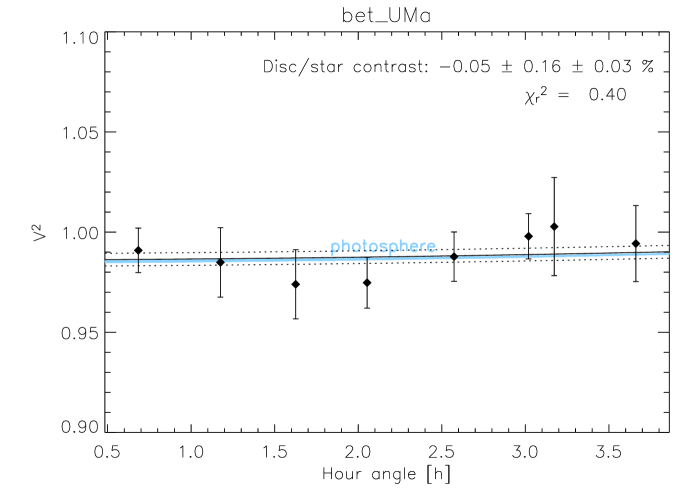
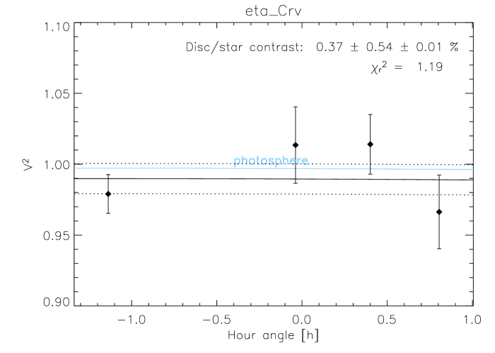
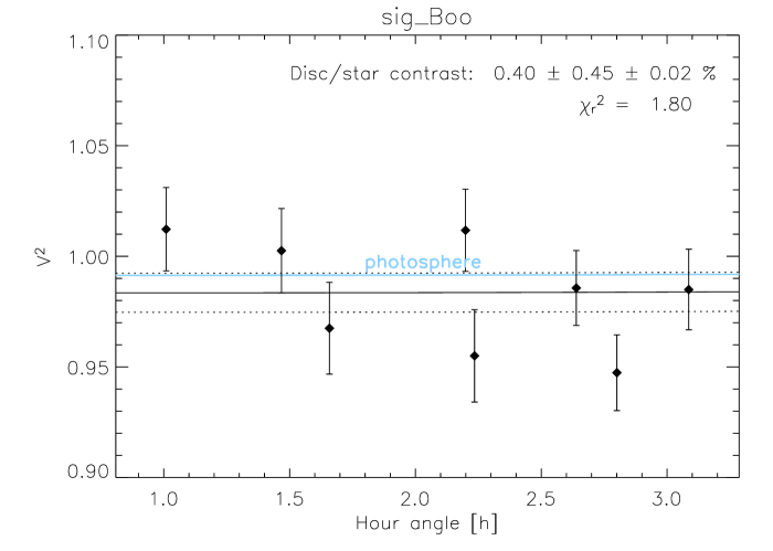
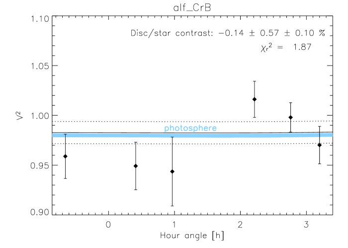
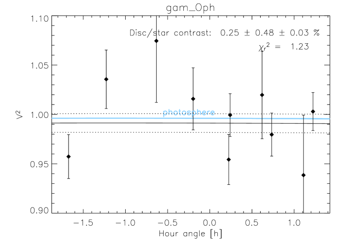
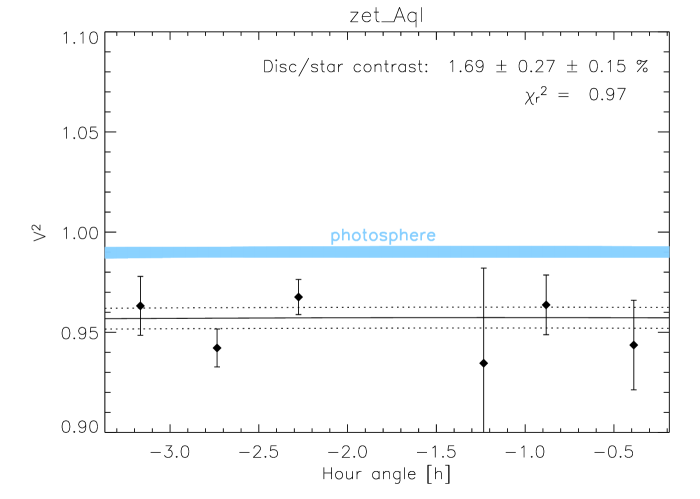
Figure 1: Squared visibilities with error bars as a function of hour angle, recorded for our six targets on the CHARA S1–S2 baseline. The blue region represents the 1$\sigma$ box defined by our photospheric models. We have fitted to our data a model of a limb-darkened photosphere surrounded by a uniform circumstellar emission. The best-fit model is represented by the black solid line, while the dotted lines represent the 1$\sigma$ statistical uncertainty on the best-fit model. Circumstellar emission is detected when the blue region lies significantly above the uppermost dotted line. The inferred contrast between the uniform circumstellar emission and the star is given as inset for each star (“disc/star contrast”), together with its two error bars (the first one is related to the statistical dispersion of the calibrated data set and the second one to the uncertainty on the photospheric model) as well as the reduced $\chi^{2}$ of the fit.

5.1 Data quality and fitting procedure

The calibrated ${\cal V}^{2}$ have been overlaid on the plots of the expected photospheric visibilities in Fig. 1. The quality of the data, which can be estimated by the size of the error bars and the dispersion of the data points, is not uniform for all targets, and depends mostly on the stellar magnitude and on the seeing conditions during the observations. The low SNR obtained on individual measurements for the faintest targets ($\eta$ Crv, $\sigma$ Boo and $\gamma$ Oph) leads to the largest error bars (typically ranging between 2% and 4% for these targets, depending on the particular conditions of the observations). The error bars for the brightest targets typically range between 1% and 2%. The statistical dispersion of the data points shows a healthy behaviour for all targets, as will be confirmed by the values of the reduced $\chi^{2}$ obtained when fitting the data with a simple star+disc model. The relatively large scatter in the $\alpha$ CrB data is due to poor seeing conditions (estimated $r_{0}\simeq 4.5$ cm) on the night this target was observed.

The calibrated ${\cal V}^{2}$ data have been fitted with a model consisting of a limb-darkened stellar photosphere surrounded by a uniform circumstellar emission filling the whole field-of-view of the instrument. To account for stellar oblateness in our fit, we have defined for all baseline orientations a mean photospheric diameter as the arithmetic mean of the angular diameters in the “large diameter” and “small diameter” cases (which both depend on the orientation of the projected baseline). The only parameter to be fitted is then the flux ratio $\epsilon_{\rm CSE}$ between the integrated circumstellar emission and the photosphere. The results of the fitting procedure are displayed as insets in Fig. 1 together with the reduced $\chi^{2}$. The first term in the error budget accounts for the statistical dispersion of the data, while the second term is related to the uncertainty on the photospheric model, which includes the uncertainties on both the surface-brightness model and the orientation of the stellar rotation axis.

5.2 Results

Among the seven early-type stars that have been surveyed so far, two stars ($\zeta$ Aql and $\alpha$ Lyr) show evidence for the presence of circumstellar emission: the fit to their interferometric measurements falls significantly below the expected squared visibility of the photosphere (see Fig. 1 and Fig. 2). The five remaining stars in our sample show no evidence for circumstellar emission: the estimated flux ratio $\epsilon_{\rm CSE}$ between the integrated circumstellar emission and the photosphere ranges between $-0.3\sigma$ and $+0.9\sigma$, where $\sigma$ represents the square sum of the statistical and systematic errors bars displayed in Fig. 1. It must be noted that our non-detections have a statistically-speaking healthy behaviour, with a mean $K$-band excess amounting to $0.3\sigma$ and a standard deviation of $0.6\sigma$. This gives us good confidence in our positive detections, which are obviously not related to a systematic effect since our stellar sample is quite homogeneous in spectral types and magnitudes. The range of values for the reduced $\chi^{2}$ of the fits is satisfactory for all cases. Let us discuss the most interesting targets individually.

$\zeta$ Aql.

Our analysis of the new CHARA/FLUOR data brings to light the presence of circumstellar emission around $\zeta$ Aql (see Fig. 1). The quality of the fit for $\zeta$ Aql is quite good ($\chi^{2}_{r}=0.97$), and the final value for the $K$-band flux ratio is $1.69\%\pm 0.31\%$, which represents a 5.5$\sigma$ detection. This result does not strongly depend on the actual limb darkening coefficient $u_{K}$ of the $\zeta$ Aql photosphere: when using extreme values of 0.0 and 0.5 for $u_{K}$, the final value for the $K$-band excess varies only from 1.68% to 1.72%. As discussed by Absil et al. (2006), this estimation of the $K$-band flux ratio does not depend on the morphology of the circumstellar emission to the first order, as long as it has an extension larger than the angular resolution of the interferometer (about 7 mas in the $K$ band for a 34-m baseline).

$\alpha$ CrB.

Let us assess whether the eclipsing binary nature of the object could significantly affect our measured visibilities. To reduce as much as possible the effect of the companion on the measured visibilities, we have used the well-characterised ephemeris of the system (Schmitt 1998) to schedule the observations of $\alpha$ CrB during an eclipse. As discussed in Sect. 4.1, the expected $K$-band magnitude difference between $\alpha$ CrB A and its companion is $\Delta K=3.25$, which is equivalent to a contrast of about 5%. The companion could thus potentially be at the origin of the fluctuations of about 10% observed in the calibrated squared visibilities. While the secondary eclipse would have been ideal to suppress the effect of the companion, time and weather constraints have forced us to observe the system during primary eclipse (when the companion passes in front of the primary). The $\alpha$ CrB system was observed on April 30th from 8:10 UT to 12:04 UT, while the primary eclipse took place between 6:56 UT (start of ingress) and 21:19 UT (end of egress). Totality of the eclipse actually started at 9:36 UT, so that part of the observations were obtained during ingress. Assuming that the companion is a standard G5V star (see Sect. 4.1), and using for the primary the linear radius of $2.94\,R_{\odot}$ deduced from the surface-brightness relationships, the diameter ratio between the two components is equal to 0.31. With the estimated $K$-band contrast, the expected variation of squared visibility for the binary system on the S1-S2 baseline between the start of ingress and the totality is only about 0.6%. This effect is clearly not sufficient to explain the dispersion of the data points, which is more likely related to the poor atmospheric conditions during the night of April 30th. Due to our optimised observation timing, the presence of the companion does not bias the search for a circumstellar excess at a level larger than about 0.2% on the disc/star contrast.

$\eta$ Crv.

The absence of significant $K$-band excess around this target comes rather as a surprise, since previous mid-infrared observations have suggested the presence of warm dust (Wyatt et al. 2005), and subsequent modelling an LHB-like event (Wyatt et al. 2007). However, we note that (i) the latest model of the $\eta$ Crv circumstellar disc predicts a contrast larger than 1:$10^{5}$ in the $K$ band between the disc and the photosphere (Smith et al. 2008) and (ii) the small number of data points that we have obtained on this target does not allow a high sensitivity to be reached (only 1:62 at $3\sigma$). Therefore, our non-detection is not incompatible with previous measurements and models, and shows that the presence of warm dust is not necessarily accompanied by large amounts of hot dust.

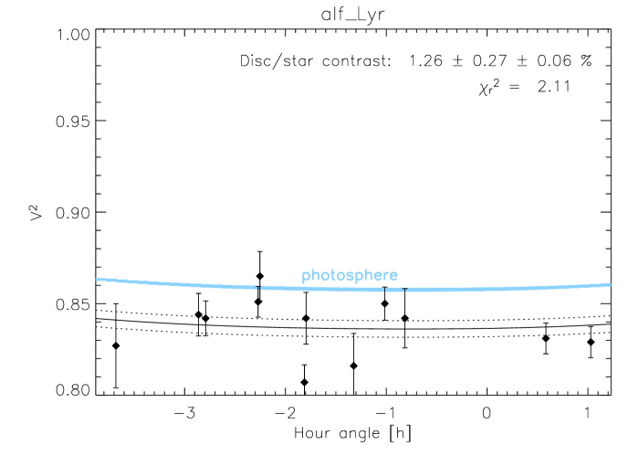
Figure 2: Same as Fig. 1 in the case of $\alpha$ Lyr. The previously published data have been re-reduced with the latest version of the FLUOR Data Reduction Software to produce this plot, using the latest limb-darkened photospheric model of Aufdenberg et al. (2006) as a reference.

$\alpha$ Lyr.

The data collected in 2005 on $\alpha$ Lyr have been re-reduced with the latest version of the FLUOR DRS, and using a more realistic model for the stellar photosphere based on the Aufdenberg et al. (2006) model (a simple uniform disc model was used in the original study by Absil et al. 2006). The new fit, displayed separately in Fig. 2, shows a good agreement with the previously published $K$-band excess ($1.29\%\pm 0.19\%$). Only the error bar on the disc/star contrast has significantly changed, due to the slightly larger error bars obtained on individual data points with the latest version of the FLUOR DRS. The contribution of the uncertainty on the photospheric model is negligible (0.06%) thanks to the accurate stellar model derived from long-baselines measurements. The agreement between the result presented here and the original disc/star contrast estimation can be seen as a welcome consistency check, since a new version of the FLUOR DRS was used to reduce the data and a more realistic stellar model was adopted. This also shows that the details of the photospheric model do not matter at the short baselines considered here.

6 Possible nature of the circumstellar emission around $\zeta$ Aql

The nature of the circumstellar emission detected around $\alpha$ Lyr has already been discussed by Absil et al. (2006), showing that the presence of hot circumstellar dust is the most probable explanation. Here, we focus on the new detection ($\zeta$ Aql), and extend our analysis to other potential contributors to circumstellar emission, including stellar winds and mass loss events. The following discussion is based on our interferometric observations, complemented only by archival infrared photometric measurements. In Sect. 7, we will include additional data from other instruments to further constrain the nature of the circumstellar emission. In this way, we want to make clear what type of information can actually be derived from a limited amount of squared visibilities obtained on a short two-telescope baseline.

The only strong constraints that we derive on the circumstellar emission from our interferometric measurements is that it represents 1.69% of the stellar flux in $K$ band and that it is located within the FLUOR field-of-view, which has a FWHM of $0\aas@@fstack{\prime\prime}8$. Due to the quasi-Gaussian beam of the FLUOR single-mode fibres, circumstellar emission located at the edge of the field (e.g., dust ring or point-like source) needs to be significantly brighter than 1.69% to produce the detected visibility deficit. Taking the transmission at the centre of the field as a reference, only half of the flux emitted at $0\aas@@fstack{\prime\prime}4$ (i.e., at a projected distance of 9 AU) makes it through the fibre’s transmission pattern. At 30 AU, the flux transmission decreases to 10%, following the theoretical Gaussian profile.

6.1 The debris disc scenario

The first scenario that we wish to investigate is the presence of hot circumstellar dust within the field-of-view of the FLUOR instrument, which would be at the origin of the measured visibility deficit. Although the origin and survival of hot dust grains close to an early-type MS star is a matter of debate, a plausible debris disc model, reproducing the interferometric measurements as well as archival photometric measurements in the near- and mid-infrared has been proposed for $\alpha$ Lyr (Absil et al. 2006). In that paper, we also showed that the actual morphology of the circumstellar dust disc does not have a significant influence on the visibility deficit measured by CHARA/FLUOR: only the flux ratio between the integrated disc emission and the stellar photosphere actually matters.

In this section, we investigate whether a debris disc model similar to that proposed for $\alpha$ Lyr would be suitable to reproduce the available measurements of $\zeta$ Aql. The purpose is not to propose a “best-fit” set of physical parameters for the dust disc, but only to check whether there exists at least a debris disc model consistent with the near- and mid-infrared observations of $\zeta$ Aql. The question of the origin and physical properties of such dust grains will be discussed in a forthcoming paper.

To perform our simulations, we have complemented our direct measurement of the $K$-band excess flux with archival spectro-photometric measurements at near- and mid-infrared wavelengths (see Table 4). In addition to the measurements found in the literature, we have used an IRS spectrum found in the Spitzer archives, which we have reduced with the c2d pipeline developed by Lahuis et al. (2006). The spectrum has been binned into a few equivalent broad-band photometric measurements for the sake of SED modelling (see Table 4). Because all these fluxes are valid for the whole star/disc system, they have been converted into an estimated excess flux by subtracting the photospheric flux. The photospheric emission model is chosen from the NextGen grid (Hauschildt et al. 1999), using stellar parameters as close as possible to the parameters estimated by Gray et al. (2003) and Adelman et al. (2002), i.e., $T_{\rm eff}=9200$ K, $\log g=4.00$ and ${\rm M}/{\rm H}=0.0$. The NextGen model is scaled to match the observed $V=2.988$, which results in an estimated luminosity of $39L_{\odot}$, in agreement with the estimation of Malagnini & Morossi (1990). We have estimated the error on the NextGen photospheric infrared fluxes by comparing neighbouring models on the NextGen grid corresponding to the typical range in $T_{\rm eff}$ and $\log g$ estimations found in the literature. Assuming effective temperatures comprised between 9200 K and 9400 K, and surface gravities between 3.5 and 4.0, we have derived a typical error of 2% on the estimated fluxes between 1 $\mu$m and 32 $\mu$m.

Table 4: Available constraints on the near- and mid-infrared photometry of $\zeta$ Aql. References: (1) Morel & Magnenat (1978); (2) Leggett et al. (1986); (3) Egan et al. (2003); (4) Chen et al. (2005). The archival Spitzer-IRS spectrum has been binned into a few photometric data points. Photometric data have been compared to our NextGen photospheric model of $\zeta$ Aql to derive fractional excesses, taking into account the typical uncertainty of 2% on the photospheric flux in the infrared (this uncertainty has been added to the estimated errors on the measured fluxes to compute the errors on the excesses).

Wavelength	$F_{\rm meas}$ (Jy)	Excess	Ref.
1.2 $\mu$m	$112.4\pm 4.1$	$-4.5\pm 5.5$%	(1)
1.24 $\mu$m	$114.5\pm 2.1$	$2.0\pm 3.9$%	(2)
2.13 $\mu$m	—	$1.69\pm 0.31$%	CHARA/FLUOR
4.35 $\mu$m	$13.3\pm 1.7$	$-2.3\pm 14.7$%	(3)
5.5 $\mu$m	$9.18\pm 0.42$	$5.3\pm 6.8$%	IRS spectrum
7.5 $\mu$m	$4.85\pm 0.22$	$1.7\pm 6.6$%	IRS spectrum
8.28 $\mu$m	$4.34\pm 0.18$	$9.5\pm 6.5$%	(3)
12.13 $\mu$m	$2.15\pm 0.13$	$14.8\pm 8.9$%	(3)
12.5 $\mu$m	$1.73\pm 0.10$	$-1.8\pm 7.6$%	IRS spectrum
14.65 $\mu$m	$1.44\pm 0.10$	$12.1\pm 9.8$%	(3)
18 $\mu$m	$0.868\pm 0.051$	$2.0\pm 8.0$%	IRS spectrum
24 $\mu$m	$0.475\pm 0.048$	$-0.7\pm 12.0$%	(4)
32 $\mu$m	$0.270\pm 0.025$	$0.8\pm 11.5$%	IRS spectrum

Our debris disc model is an adaptation of the “best-fit” model that we derived in the case of $\alpha$ Lyr (Absil et al. 2006), based on the model of Augereau et al. (1999). It assumes a size distribution $dn(a)\propto a^{-3.7}da$ with limiting grain sizes $a_{\rm min}=0.1$ $\mu$m and $a_{\rm max}=1500$ $\mu$m, a surface density power-law $\Sigma(r)\propto r^{-4}$, and chemical composition of 50% amorphous carbon and 50% glassy olivine. The inner radius of the dust distribution has been recomputed in a similar way as in the case of $\alpha$ Lyr, and is found to be equal to 0.14 AU. This corresponds to the sublimation radius for the grains larger than about 1 $\mu$m, while 0.1 $\mu$m grains sublimate at $\sim 0.45$ AU in the model. All grains within their sublimation distance are self-consistently eliminated from the simulations, leading to regions around the inner disc edge depleted in submicronic grains. The only free parameter is the total mass of the disc, which has been adjusted to the photometric and interferometric data in Fig.3. With a reduced $\chi^{2}$ of 0.54, our model does a good job in reproducing the global SED of $\zeta$ Aql from 1 to 32 $\mu$m, and demonstrates that the presence of hot dust, with a total dust mass of only $5.5\times 10^{-8}$ M_⊕ and a fractional luminosity of about $10^{-3}$, is a viable explanation to the observed $K$-band excess. It must be noted that, as in the case of $\alpha$ Lyr, most of the grains in this model are submicronic and located close to their sublimation radius. Possible scenarios to explain the presence of such grains have already been proposed (Absil et al. 2006) and will be further discussed in a forthcoming paper.

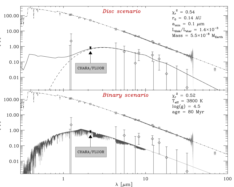
Figure 3: Top panel: A possible fit of our debris disk model to the photometric and interferometric constraints of Table 4. The dashed line represents the contribution of thermal emission to the overall disc emission, while the solid line includes the scattered light contribution. Photometric measurements are represented by squares with error bars, and the related excesses by diamonds. The CHARA/FLUOR interferometric measurement is represented by a filled circle with error bar. The whole IRS spectrum is represented by a grey box with a width equal to its error bar, and was converted into a few regularly spaced (in log scale) broad-band photometric measurements for the fitting procedure. The MIPS photometric measurement at 70 $\mu$m (Chen et al. 2005) is also represented but was not included in the fit. Bottom panel: Same figure in the case of a low-mass companion. The spectrum of the companion is represented by a NextGen model (Hauschildt et al. 1999) where the stellar parameters ($T_{\rm eff}=3800$ K, $\log g=4.5$) have been chosen as close as possible to our best-fit model (see Sect. 6.3). The resolution of the NextGen spectrum of the A0-type host star has been degraded by a factor 20 in both panels for the sake of clarity.

The hot debris disc model proposed for $\zeta$ Aql can further be used to derive upper limits on the mass of hot dust around the stars in our sample for which no detection was reported. This estimation is based on the fact that none of the surveyed stars shows a significant photometric infrared excess in the 1–5 $\mu$m region, and on the fact that their spectral types are close enough for the same debris disc model to apply to all of them. Noting that the final error bar on the disc/star flux ratio is typically 0.5% for these stars (except for $\beta$ UMa, which has a significantly lower error bar of 0.16%), we derive a typical $3\sigma$ upper limit of $5\times 10^{-8}$ M_⊕ for the hot dust content within the FLUOR field-of-view of $0\aas@@fstack{\prime\prime}8$ (i.e., 18 AU at the mean distance of our sample). Scaling this mass to the smaller error bar of $\beta$ UMa gives a $3\sigma$ upper limit of $1.5\times 10^{-8}$ M_⊕ for this particular system. We note that our observations are only sensitive to hot dust, and that larger amounts of colder dust could be present, especially beyond a few AUs where equilibrium temperatures are significantly smaller than 1000 K (see e.g. the discussion of $\eta$ Crv in Sect. 5.2).

6.2 Stellar wind and mass loss

With their relatively high masses and high rotational velocities, one may think that our target stars could be the subject of significant mass loss or winds that could, as in the Be phenomenon, lead to a substantial near-infrared emission in addition to the photospheric level. However, winds of A-type stars are actually suspected to be very weak, as the mechanisms which are efficient in both later type stars and earlier ones are not expected to operate on A-type stars: radiative pressure is very small (compared to B-type stars), and there is no deep convection giving rise to activity phenomenon as in late-type stars (Babel 1995). Convection is actually expected to start for effective temperatures below 6500 K (Lamers & Cassinelli 1999), i.e., for spectral types later than about F6 V, so that A-type stars are not expected to have chromospheres and coronae. This fact seems to be corroborated by the lack of observational evidence for winds emanating from A-type stars (Lanz & Catala 1992; Landstreet et al. 1998), as well as by the absence of X-ray emission from most A-type stars (Schröder & Schmitt 2007).

Nonetheless, we note that the presence of a stellar wind has been detected around Sirius (A1 V) through the observation of an absorption feature in the blue wings of the Mg II and H I resonance lines (Bertin et al. 1995). The inferred mass-loss rate ranges between $2\times 10^{-13}$ and $1.5\times 10^{-12}M_{\odot}{\rm yr}^{-1}$, and has not been shown to produce any significant near-infrared emission. Based on radiatively driven wind models, Babel (1995) predicts much lower mass loss rates ($<10^{-16}M_{\odot}{\rm yr}^{-1}$), with winds consisting of only metals. Additionally, the infrared excess that could be associated to the winds from hot stars is expected to originate mostly from a region $R<1.5R_{\ast}$ (Lamers & Cassinelli 1999), which does not match our observations because such a compact emission would not produce a significant visibility reduction at the short baselines used here.

Intriguingly, shell lines of Ti II have been detected by Abt et al. (1997) in the ultraviolet spectra of approximately one-quarter of the most rapidly rotating normal A-type dwarfs ($v\sin i\geq 200$ km s^-1). In that paper, the authors suggest that this “hot disc” phenomenon might be related to sporadic mass-loss events and does not seem to correlate to the presence of cold dust in an outer debris disc. However, more recently, Abt (2004) and Abt (2008) have argued that these hot discs are actually accreted from the interstellar medium. The argument is based on the fact that such discs rarely occur around stars within the heart of the Local Interstellar Bubble (LIB). The author proposes a model in which stars accrete discs in dense interstellar regions, but loose them in regions of low interstellar density, such as the LIB, where the stellar winds exceed the accretion rate. The spectral lines associated with the hot disc disappear on timescales of roughly decades. Since our target stars are all located well within the LIB ($\ll 100$ pc), this phenomenon does not seem appropriate to reproduce our observations.

All these elements indicate that a stellar mass-loss origin to the observed near-infrared excess is highly unlikely in the case of A-type dwarfs. Furthermore, we have examined archival HARPS data on $\zeta$ Aql and found no sign of H$\alpha$ emission, which accompanies strong stellar winds produced by hot stars. The stellar wind scenario will thus be discarded in the rest of the discussion.

6.3 Point-like source

Because of our sparse sampling of spatial frequencies, we cannot determine the actual morphology of the excess emission source, and a point-like source located within the FLUOR field-of-view (either a bound companion or a background source) could be at the origin of the observed visibility deficit. To assess the effect of a faint companion on the measured visibilities, two cases must be considered, depending whether the two fringe packets are superimposed or not. Taking into account the coherence length of the FLUOR fringes (about 25 $\mu$m), the minimum on-sky angular separation for two separated fringe packets is 150 mas along the baseline direction, i.e., about 3.5 AU at the distance of $\zeta$ Aql. For larger separations, the off-axis point-like source contributes essentially as an incoherent emission and produces a squared visibility deficit $\Delta{\cal V}^{2}=2f$, where $f$ is the flux ratio between the primary and the secondary. A point-like source within the FLUOR field-of-view, located at a distance larger than 150 mas from $\zeta$ Aql in the projected direction of the interferometric baseline and producing 1.69% of the photospheric flux of $\zeta$ Aql, would therefore be a possible explanation to the measured visibility deficit.

Let us now investigate the case of a close companion ($<150$ mas), for which the two fringe packets would be superposed. In that case, the companion produces a modulation in the fringe visibility depending on its position and on the geometry of the array, which changes as the Earth rotates. The squared visibilities are therefore expected to be modulated as a function of the hour angle of the observation. To determine which combination of angular separation and position angle would be compatible with the interferometric observations, we compute the squared visibilities for a binary system at various distances and position angles, assuming that the off-axis source did not move during the 11 nights of our May 2006 observing run. For each given position, the contrast between the two components is then adjusted to minimise the $\chi^{2}$ distance between the synthetic and measured squared visibilities. In this way, we produce a $\chi^{2}$ map, taking into account the wide bandwidth effect of the FLUOR instrument.

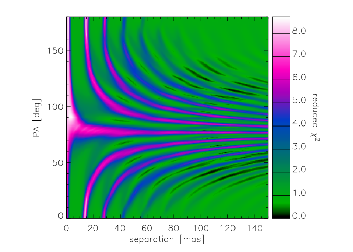
Figure 4: Map of the reduced $\chi^{2}$ distance between a binary star model and our CHARA/FLUOR squared visibilities for $\zeta$ Aql, as a function of the position of the faint companion. The binary flux ratio has been adjusted separately at each given position to minimise the $\chi^{2}$. Dark regions indicates binary solutions compatible with the CHARA/FLUOR data.

The $\chi^{2}$ map, represented in polar coordinates in Fig. 4, indicates that many different locations of the off-axis point-like source may reproduce the squared visibilities measured by CHARA/FLUOR. In particular, for any given angular separation larger than 3 mas, we can always find a position angle that makes the simulated data compatible with the observed visibilities (reduced $\chi^{2}\lesssim 1$). We also note that the optimum binary flux ratio at the positions where the reduced $\chi^{2}$ is smaller than 2 is in excellent agreement with the “disc/star” contrast computed in Sect. 6.1: the mean flux ratio at such locations is 1.65%, with a standard deviation of only 0.22%. This further confirms that the morphology of the circumstellar emission does not have a significant influence on the inferred flux ratio, and indicates that the simplified computation of the binary flux ratio assuming separated fringe packets can also be used as a good approximation for superposed fringe packets.

Figure 4 is also a nice illustration of the wide bandwidth effect in optical interferometry: for position angles parallel to the mean baseline orientation (i.e., ${\rm PA}=170^{\circ}$), one can see that the ripples in the $\chi^{2}$ map due to the visibility modulation produced by the binary star progressively wash out as the companion moves away from the primary star. This effect can be interpreted as the progressive separation of the two fringe packets. The reduced $\chi^{2}$ values obtained at a position where the fringe packets are essentially separated (i.e., separation of 150 mas and position angle close to $170^{\circ}$) make a nice connection with the case of large separations described earlier in this section. One can also note that for position angles perpendicular to the mean baseline azimuth, the reduced $\chi^{2}$ does not change significantly as a function of distance, because only the projection of the angular separation along the baseline direction actually matters.

Finally, we have checked that we can find on the NextGen stellar atmosphere grid a low-mass stellar companion compatible in terms of flux both with our CHARA/FLUOR measurement and with the archival photometric data listed in Table 4. In the bottom panel of Fig. 3, we show that an M0V-type star with $T_{\rm eff}=3800$ K and $\log g=4.5$ nicely fits the whole data set. A low-mass companion located at an angular distance larger than 3 mas from the central star is therefore a plausible explanation to the observed visibility deficit at short baselines.

7 Discussion

Our interferometric observations are not sufficient to determine the morphology of the circumstellar emission. In this section, we investigate whether complementary data obtained with various types of instruments could further constrain the nature of the circumstellar excess.

7.1 Further constraints on the debris disc scenario

The identification of $\zeta$ Aql as a debris disc star by Chen et al. (2006) was based on the measurement of significant excess emission on top of the expected photospheric flux at 12 and 24 $\mu$m. However, Fig. 3 strongly contradicts this statement, and shows the absence of cold circumstellar dust at the sensitivity limit of the Spitzer IRS and MIPS instruments. The discrepancy with the analysis of Chen et al. (2006) is related to the effective temperature of 11912 K that they have used to compute the photospheric emission of $\zeta$ Aql, which does not match the estimated temperatures found in the literature, ranging between 9190 and 9680 K (see e.g. Gray et al. 2003; Adelman et al. 2002; Malagnini & Morossi 1990). Only the polar temperature could reach such a high value (Peterson et al. 2006a), while $\zeta$ Aql is view essentially equator-on. The very good match between our photospheric emission model and the IRS spectrum gives us a high confidence in our flux estimation, and clearly shows that no excess emission is detected in the 24–70 $\mu$m region. This also explains why a black body disc model did not allow Chen et al. (2005) to consistently reproduce the 24 and 70 $\mu$m excesses that they had derived. The fact that the MIPS 70 $\mu$m measurement falls about $3\sigma$ below our photospheric model (see Fig. 3) could be either due to a poor flux calibration on this target or to an underestimated error bar.

Despite the absence of observable amounts of cold dust, the presence of hot circumstellar dust in the close neighbourhood of 83 Myr old A-type star could still be explained in the context of terrestrial-planet formation models. In particular, Kenyon & Bromley (2006) describe oligarchic and chaotic growths in the terrestrial region around a solar-type star, and show that the planet formation timescale is 10–100 Myr (see also Chambers 2004, and references therein). The onset of chaotic growth depends on the surface density, and typically ranges between 0.1 Myr and a few Myr. During the subsequent chaotic phase, the dynamical perturbations between oligarchs may lead to enhanced dust production. This potential origin for the dust observed around $\zeta$ Aql is also supported by the study of Rieke et al. (2005), who suggest that the dust detected towards relatively young A-type stars may be related to the planet accretion end game. According to Chambers (2001), the accretion end game is predicted to be dominated by a small number of collisions between large bodies (e.g., the early Earth and the impactor that caused formation of the Earth’s Moon) and may stretch over 100–200 Myr. Kokubo et al. (2006) also show that the giant impact stage (i.e., the accretion timescale) around a Solar-type star lasts for about 100 Myr. However, it must be noted that, according to Kenyon & Bromley (2004), the major part of the warm infrared excess may disappear within 1–10 Myr during terrestrial planet formation around Sun-like star. Furthermore, Kenyon & Bromley (2005) show that, in the case of a 3–20 AU region around A-type stars, 1000 km objects are formed within 10 Myr, the dust luminosity peaks at 1 Myr and is already at a very low level at 100 Myr.

In conclusion, even though the presence of hot dust in the close environment of $\zeta$ Aql cannot be ruled out, the likeliness of this scenario can be questioned due to the absence of a large reservoir of cold dust in the outer planetary system.

7.2 Further constraints on the binary scenario

To get a better grasp at the possible nature of the potential point-like source around $\zeta$ Aql, we compute the flux of the hypothetical companion reproducing the observed visibility deficit as a function of its distance, taking into account the Gaussian off-axis transmission of the single-mode fibre. For the sake of clarity, the apparent binary flux ratio seen through the Gaussian transmission pattern is approximated by the simple expression ($f=\Delta{\cal V}^{2}/2$), which strictly applies only to wide binaries ($>150$ mas), even though we have shown in Sect. 6.3 that this relationship is a good approximation to the best-fit solutions for close binaries. The derived flux ratio is then converted into the mass of the hidden companion in Fig. 5 (solid line) as a function of linear distance to the central star, using the mass-luminosity relationships of Baraffe et al. (1998).

As already discussed by Absil et al. (2006) and Paper I, the presence of a background source producing such a flux within the $0\aas@@fstack{\prime\prime}8$ FLUOR field-of-view is highly unlikely. Therefore, we investigate here the possible presence of a bound companion around $\zeta$ Aql. Although $\zeta$ Aql is known to be part of a wide multiple system (ADS 12026), its detected companions are no closer than $5\arcsec$ so that they cannot affect our visibility measurements. This star is classified as a spectroscopic binary in the WDS catalogue. However, this classification is most probably wrong as it is based on a measurement from the late 19th century, which has not been confirmed since then. The detection of X-ray emission towards $\zeta$ Aql with ROSAT is a possible sign for the presence of a low-mass companion (Schröder & Schmitt 2007). However, due to the large PSF of the ROSAT satellite ($18\arcsec$), the visual companion that was located at $6\aas@@fstack{\prime\prime}5$ from $\zeta$ Aql in 1934 according to the WDS catalogue could be at the origin of the observed X-rays. To our knowledge, no other sign of the presence of a close companion to $\zeta$ Aql has been reported in the literature. However, close and faint companions are difficult to detect.

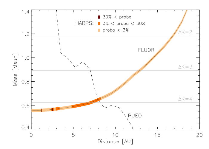
Figure 5: Constraints on the mass and distance of a hypothetic companion around $\zeta$ Aql. The solid line, labelled FLUOR, represents the solutions that are compatible with our interferometric observations. The adaptive optics images that we have obtained with PUEO constrain the companion to be located below the dashed line (PUEO $3\sigma$ detection limit). The probability that the companion defined by the FLUOR curve fits our HARPS data is represented by three colour levels along the FLUOR curve. The correspondance between the mass of the companion and its $K$-band contrast with respect to the primary is indicated by grey horizontal lines, based on the evolutionary models of Baraffe et al. (1998).

In order to improve our knowledge of the close environment of $\zeta$ Aql, deep adaptive optics images have been obtained in the $K$ band with the PUEO instrument at the Canada-France-Hawaii Telescope. Under good seeing conditions (about $0\aas@@fstack{\prime\prime}6$), no companion was detected at the sensitivity limit of the instrument ($\Delta K=4$ at $0\aas@@fstack{\prime\prime}3$, and improving for larger separations). The $3\sigma$ sensitivity to point-like companions has been computed as a function of angular separation and has been converted into the maximum mass of a hidden companion in Fig. 5 (dashed line) as a function of linear distance, using the mass-luminosity relationships of Baraffe et al. (1998). All solutions with companions orbiting further than about 8 AU can be discarded by the PUEO observations, but closer companions are not constrained.

We have therefore used radial velocity data obtained with HARPS to further constrain the possible presence of a low-mass companion around $\zeta$ Aql. We have tried to fit simple orbital solutions to the HARPS data collected between 2004 and 2008 (represented in Fig. 6), assuming a 90^∘ inclination for the binary system and a zero eccentricity. Each point along the FLUOR curve in Fig. 5 defines a single couple “period – maximum radial velocity”, which is computed with classical orbital dynamics relationships and defines the shape of the sinusoidal radial velocity curve. For each couple “period – velocity” on the FLUOR curve, we have computed the $\chi^{2}$ between the observed HARPS data and a series of sinusoidal models with various time and radial velocity offsets. The lowest $\chi^{2}$, associated to the best-fit offsets in time and radial velocities, has then been converted into a probability, which represents the likeliness that the binary star model actually reproduces the HARPS data. Probabilities are represented by three colour levels in Fig. 5, and show that two solutions at orbital radii $a=1.2$ AU and $a=2.5$ AU are most probable (i.e., 47 mas and 98 mas respectively). The potential companions have respective masses of 0.56 and $0.57\,M_{\odot}$ and complete their orbits in 280 and 842 days. These two most probable solutions are respectively represented by solid and dotted curves in Fig. 6. The closest model on the Baraffe et al. (1998) evolutionary grid at 80 Myr for these two potential companions is a $0.57\,M_{\odot}$ object with an effective temperature $T_{\rm eff}=3779$ K and a surface gravity $\log g=4.68$. Its absolute magnitude is $M_{K}=5.22$, giving $K=7.26$ at the distance of $\zeta$ Aql, and thus a $\Delta K=4.36$ with the primary. The associated $V$-band magnitude is 11.2, so that the contrast with the primary is $\Delta V=8.2$.

Even though the HARPS data do not give a definitive answer regarding the orbital parameters of the putative companion, we must recognise that the absence of a bound companion seems rather unlikely based on the HARPS data alone: when fitting the HARPS data with a constant velocity, the reduced $\chi^{2}$ with 9 degrees of freedom is equal to 3.6, and the associated probability that the model represents the data is of only 0.02%. Nevertheless, this result depends essentially on two HARPS radial velocity measurements with values around 5000 m/s in the middle of Fig. 6, and a better time sampling would be needed to confirm the detection of the putative companion. It must finally be noted that stellar pulsations are not expected to produce such radial velocity variations in the case of $\zeta$ Aql, a main-sequence A0 star not classified as a $\delta$ Scuti variable.

Figure 6: Radial velocities measured on $\zeta$ Aql with HARPS during the past 4 years. The two most probable circular orbits compatible with both the HARPS data and the FLUOR constraints have been overlaid as solid and dotted curves.

A last constraint that we can put on the potential low-mass companion is that it must comply with the astrometric stability of $\zeta$ Aql: Hipparcos observed this star on about 20 different occasions between March 1990 and March 1993 (total time span of 1000 days), and found no sign of binarity at an astrometric accuracy of 0.72 mas (Perryman et al. 1997). Taking an estimated mass of $0.57\,M_{\odot}$ for the companion, this basically rules out any circular binary solution with a semi-major axis larger than 0.2 AU at the $3\sigma$ level. However, if the orbital period is significantly larger than the time span of the Hipparcos observations, the presence of a low-mass companion could have been missed, all the more that the system is supposedly viewed edge-on so that the reflex motion of the primary star could have been confused with its proper motion. We estimate that binary solutions with orbital periods larger than about 3000 days, even though they are associated with astrometric signals larger than 50 mas, would not have been detected at the $3\sigma$ level by Hipparcos. This corresponds to a semi-major axis of about 5.5 AU. All solutions with semi-major axes between 0.2 AU and 5.5 AU would thus most likely have been detected by Hipparcos, and the two most probable solutions provided by the fit to the HARPS data seem incompatible with the astrometric constraints. However, we note that there remains a range of plausible solutions at semi-major axes between 5.5 AU and 8 AU, with stellar masses ranging between $0.6$ and $0.65\,M_{\odot}$. We also note that the use of eccentric orbits to fit the HARPS data could lead to significantly different orbital solutions, which may improve the compatibility with the Hipparcos constraints.

In conclusion, the presence of a bound low-mass companion can neither be confirmed nor rejected based on currently available data. We plan to obtain further observations of $\zeta$ Aql at high angular resolution with single-pupil telescopes to give a final answer to this question. In particular, the new Sparse Aperture Masking mode of the NACO adaptive optics instrument at the VLT would be perfectly suited to reach this goal. Interferometric closure phase measurements on longer baselines could also help unveiling the nature of this infrared excess.

8 Conclusion

In this paper, we have investigated the close neighbourhood ($<1\arcsec$) of six nearby A- and early F-type MS stars, in search for hot counterparts to the cold debris discs detected by mid- and far-infrared spectro-photometric space-based observations. The high-accuracy squared visibilities collected with the CHARA/FLUOR interferometer, combined with semi-empirical models of stellar photospheres including rotational distortion, has allowed us to reach dynamic ranges ranging from 1:175 to 1:625 at $1\sigma$ around the target stars. At this level of precision, the presence of a resolved $K$ band emission has been identified around only $\zeta$ Aql, with a estimated $K$-band excess of $1.69\pm 0.31$%. This detection adds to our previous results on $\alpha$ Lyr (Absil et al. 2006) and $\tau$ Cet (Paper I), giving an overall near-infrared excess detection rate of $3/9$ for the MS stars surveyed so far, among which $2/7$ are early-type stars. The healthy statistical behaviour of the five non-detections in the present sample and the confirmation of the excess emission around $\alpha$ Lyr with an improved photospheric model and a new version of the FLUOR Data Reduction Software demonstrate the robustness of our approach for hot debris disc detection.

Our near-infrared interferometric measurements are not sampling the Fourier frequency plane in a sufficiently dense manner to derive the morphology of the excess emission source. In particular, both a point-like source and an extended circumstellar emission can reproduce our observations. While in the cases of $\alpha$ Lyr and $\tau$ Cet, the presence of a bound or unbound companion to the target stars within the small FLUOR field-of-view could be rejected with a high confidence, we cannot rule out the presence of a low-mass companion in the close vicinity of $\zeta$ Aql to reproduce the measured $K$-band excess. The combination of the astrometric stability of $\zeta$ Aql measured by Hipparcos, the variability of the radial velocities measured with HARPS and the absence of off-axis companion in PUEO observations restricts the parameter space of the high-contrast binary scenario to masses in the range $0.6$ to $0.65\,M_{\odot}$ and semi-major axes between 5.5 and 8 AU (i.e., about 200 and 300 mas). The $K$-band contrast between the primary and its companion would then be $\Delta K\sim 4$, making it one of the closest high-contrast companions resolved around MS stars so far.

Besides a low-mass companion, the presence of hot circumstellar dust grains producing a significant thermal emission in the $K$ band is another viable explanation of the observed excess emission. In particular, we show that the debris disc model that Absil et al. (2006) have proposed in the context of $\alpha$ Lyr is consistent with both our $K$-band detection and archival near- and mid-infrared spectro-photometric measurements. However, our re-interpretation of archival Spitzer/MIPS and Spitzer/IRS data clearly shows that the presence of an outer debris disc, suggested by Chen et al. (2005), can be firmly ruled out at the sensitivity level of MIPS and IRS. In the absence of significant amounts of cold dust, the hot debris disc scenario is not favoured to explain our CHARA/FLUOR measurements.

The statistics of the “hot debris disc” phenomenon presently remains poorly constrained: for early-type stars, a hot debris disc was found around only one star ($\alpha$ Lyr) out of six bona fide debris disc stars observed so far. The case of $\alpha$ Lyr could therefore be rather unusual. Our interferometric survey of debris disc stars will be extended to larger sample in the coming years to improve our statistics. The case of $\zeta$ Aql must be considered separately, since we show that it is not surrounded by cold dust at the sensitivity level of the Spitzer instruments, and since a close companion is a likely explanation to the observed $K$-band excess. This star will deserve special attention in the future, and further observations will be performed to determine the actual nature of the near-infrared excess emission that we have resolved. In particular, infrared aperture masking experiments on large telescopes have the potential to reveal the true nature of the observed excess.