Crossover Between Organized and Disorganized States In Some Non-Equilibrium Systems
Abstract
We study numerically the crossover between organized and disorganized states of three non-equilibrium systems: the Poisson/coalesce random walk (PCRW), a one-dimensional spin system and a quasi one-dimensional lattice gas. In all cases, we describe this crossover in terms of the average spacing between particles/domain borders and the spacing distribution functions . The nature of the crossover is not the same for all systems, however, we found that for all systems the nearest neighbor distribution is well fitted by the Berry-Robnik model. The destruction of the level repulsion in the crossover between organized an disorganized states is present in all systems. Additionally, we found that the correlations between domains in the gas and spin systems are not strong and can be neglected in a first approximation but for the PCRW the correlations between particles must be taken into account. To find with , we propose two different analytical models based on the Berry-Robnik model. Our models give us a good approximation for the statistical behavior of these systems in their crossover and allow us to quantify the degree of order/disorder of the system.
Keywords: Systems out of equilibrium, random matrices and Berry-Robnik model.
PACS: 05.40.Fb, 05.50.+q, 45.70.Vn.
1 Introduction
Many one-dimensional non-equilibrium systems exhibit a crossover between disorganized and organized states. This crossover usually depends on the value of one or more parameters which set the system in one of these states. Our main objective is to study the statistical behavior of three non-equilibrium systems in their crossovers between organized and disorganized states. The first system is the Poisson/coalesce random walk (PCRW) where the particles describe independent random walks and when two particles meet they coalesce with probability , otherwise, they interchange their positions. The second system is a quasi one-dimensional gas, where the particles interact only by volume exclusion in presence of an external field. The last system is a one-dimensional spin lattice, where the particles interact by a coupling force in presence of an external driving field.
We propose two analytical models for the spacing distribution functions of these systems and compare them with the numerical results from the simulation. Our analytical models are based on the Berry-Robnik model introduced in Ref. [1]. This model is used in quantum systems which are neither integrable nor fully chaotic in order to find an analytical approximation to the nearest neighbor distribution of the energy levels of the system, see Refs. [1, 2, 3]. The Berry-Robnik model depends on one parameter which controls the crossover. The crossover is described through the nearest neighbor distribution , which gives us the probability that the distance between two consecutive levels is . We complement the model proposed in Ref. [1] calculating analytically the higher order spacing distribution functions for and the pair correlation function by two methods.
This paper is organized as follows. Because of its importance, in the second section we explain in detail the Berry-Robnik model. In third, fourth and fifth sections, we test our analytical models with three non-systems: the Poisson/coalesce random walk, the quasi one-dimensional gas and one-dimensional spin lattice respectively. These systems are also explained in those sections.
2 Berry-Robnik model as a non-equilibrium system
We consider a continuous one-dimensional ring with two kinds of particles and and normalized densities and respectively. The particles are subject to the reaction , i.e., they are coalescing random walkers. Particles describe independent random walks and they are subject to the reaction . The amount of particles that disappear is calculated in such way that the number of particles, , and the number of particles, , satisfy the relation at each time step. This is the only interaction between both species of particles.
For this system, is the probability that the distance between two particles is at time under the condition that between these particles there are additional particles. When the average distance between neighbor particles is much smaller than the size of the lattice, the system exhibits a dynamical scaling for all values of and . In this regime the spacing distributions can be scaled by using the variable change . Then, we obtain the time independent spacing distributions .
It is known that in the scaling regime where is the diffusion constant and is the size of the lattice, see Ref. [4] for more information about the coalescing random walk (CRW). It is straightforward to show that , then, the average length between nearest neighbors satisfy .
The interaction between species warrants that the quotient between normalized densities and is constant for all time, i.e., the rate of disappearance of particles is proportional to the one for particles and the proportionality constant is . Taking this into account, in the scaling regime, the system is the uncorrelated superposition of two independent systems of particles and with constant normalized densities. Our objective is to calculate the nearest neighbor distribution of the whole system. This can be done easily because we have the superposition of two uncorrelated distribution functions which satisfies
| (1) |
and
| (2) |
where and is the density of particles corresponding to the systems or . As is natural, the normalized densities satisfy .
Let be the probability to choose randomly an empty segment of length . This probability is related to . In order to prove that, we consider the probability that there are no particles in the interval to , given that there is a particle at . This probability is given by .
In our case we have the uncorrelated superposition of two kinds of particles, then we can write
| (3) |
where, for example, is the probability that the particle in position belongs to the system, and are the probabilities that there are no particles of the systems and in the interval, respectively. In order to find , we choose a particle randomly, the probability that the chosen point lies within a gap of length to is proportional to , to normalize this equation we use the fact that , obtaining the probability distribution . Now, the probability that the distance to the next particle is , given that the point is in the gap of length , is zero if and if . The probability of not having a particle of the system in an interval of length is ( is the unit step function).
Thus, the unconditional probability that the distance until the next particle is is given by
| (4) |
The same argument can be done for the second term of equation (3). Thus Eq. (3) takes the form
| (5) | |||||
The probability is the probability that , then, integrating Eq. (5) over we find
| (6) |
where we define
| (7) |
From equations (6) and (7), the spacing distribution function , which results of the mix of systems and is given by
| (8) |
The fact that is given by the product of functions is natural, because we used two statistical independent sequences. It is easy to prove that the functions satisfy
| (9) |
and
| (10) |
From the above equations it follows that is given by
| (11) |
Then, even if and it can happen that . In our particular case, we superpose one Wigner distribution
| (12) |
with density and one Poisson distribution
| (13) |
with density , then, we have
| (14) |
where is the density of Poisson sequence, is the one for the Wigner sequence and is the complementary Gaussian error function. Note that Eq. (14) reduces to the Poisson distribution for , and for it reduces to the Wigner distribution. This result is well-know in random matrices theory and corresponds to the Berry-Robnik model for crossover between chaotic and non-chaotic behavior in quantum systems, see Ref. [1].
2.1 Higher spacing distribution functions
In Refs. [5, 6] the authors show that the nearest neighbor distribution is not enough to describe the complete statistical behavior of a non-equilibrium system, because several different systems could share the same nearest neighbor distribution. Because of that, we generalize the Berry-Robnik model for higher spacing distribution functions. Let be the joint probability that the intervals are empty. The intervals are non overlapping and ordered . Because of the independent superposition nature of the Berry-Robnik model, can be written as
| (15) |
where and are the joint probabilities for particles and respectively. The authors of Ref. [7], showed that spacing distribution functions can be calculated from Eq. (15), let us summarize their most important result. Let be the probability that given one particle its -th neighbor is at a distance . From its definition is given by
| (16) |
with
| (17) |
On the other hand, it is well-know that for CRW, is given by [4]
| (18) |
where symbolize an ordered permutation, , of the variables , such that
| (19) |
| (20) |
In Eq. (18) is the signature of the permutation, i.e., =1 for even permutations and for odd permutations.
The function is the probability that from to the lattice is empty. Then it is possible generate the complete solution for the CRW from , which is given by the solution of the diffusion equation under the suitable boundary conditions (see Ref. [4]). In fact, the exact expression for this function is
| (21) |
for additional information see Refs. [4] and [8]. The particles describe independent random walks, then, we have
| (22) |
and
| (23) |
From equations (15), (18), (21) and (23) we can calculate for the whole system and then, we can use (16) and (17) to calculate . By using this formalism it is also possible to calculate the -point correlation function
| (24) |
in fact, the pair correlation function is given by
| (25) |
The above equation takes the form for . For we recover the pair correlation function of the CRW, see Ref [4].
3 A simple model of crossover between organized and disorganized states: The Poisson/coalesce random walk
Consider a one-dimensional ring with sites and particles, then, the particle density is given by . The particles describe independent random walks and when two particles meet they coalesce with probability , otherwise, they interchange their positions. This system was studied previously in Refs. [9, 10]. The algorithm used in the simulation is the following:
-
1.
particles are randomly inserted in a sites lattice.
-
2.
A particle is chosen at random.
-
3.
The particle can move to the left or to the right with same probability. If the particle is moved to an occupied site, the particles coalesce with probability or they interchange their positions with probability .
-
4.
In a time unit all particles are moved.
In the limit , finite systems reach a non-equilibrium steady state (NESS), where there is only one particle which executes a simple random walk and . As we will see soon, for an infinite size system in the same limit, the average length between nearest neighbor particles grows as for and the system is statistically equivalent to the CRW.
It is possible to derive an approximate analytical solution by using the inter-particle distribution function method (IPDF), see Refs. [4, 9]. Let be the probability to find an empty segment of length in the lattice. The master equation for can be written as
| (26) |
with boundary conditions and . The probability cannot be written in terms of . However in Refs. [4, 9] the authors propose an approximation for this probability
| (27) |
which can be written in terms of as
| (28) |
This approximation allows us to calculate the concentration of particles . From Eqs. (26) and (28) and summing over the index it is easy to find
| (29) |
Taking into account that and making the approximation , in Ref [9] it is found that
| (30) |
where and . Equation (30) can be integrated obtaining
| (31) |
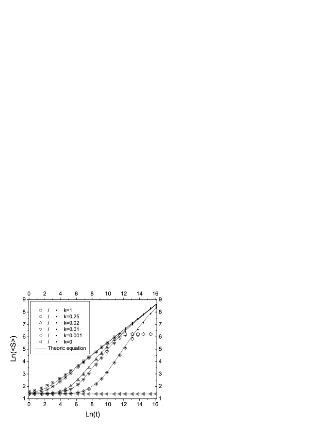
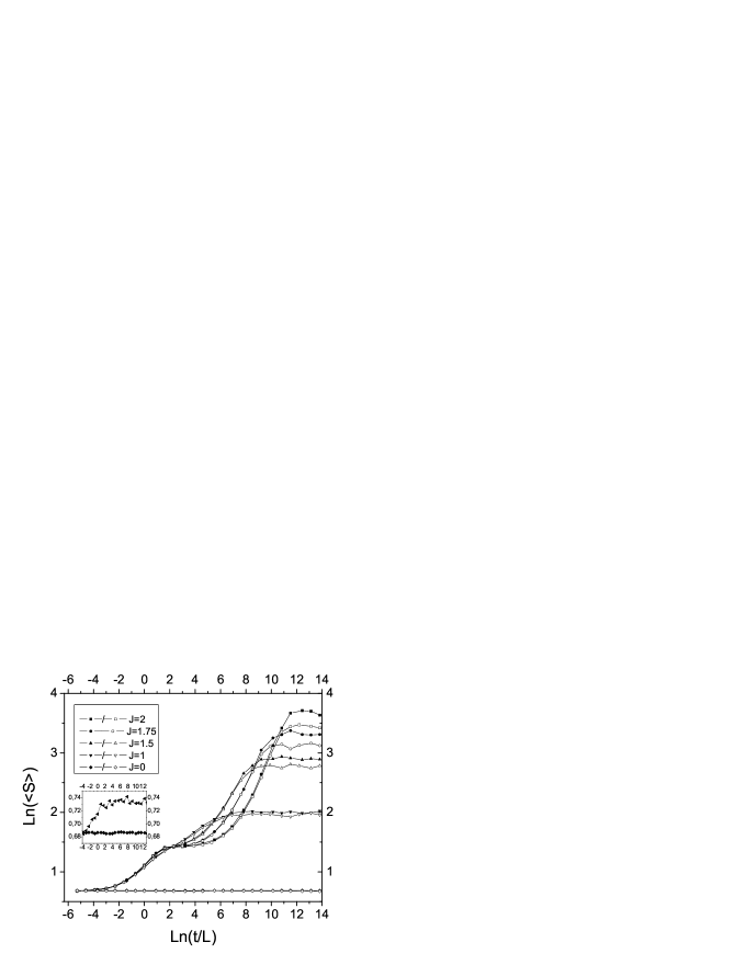
with . Note that for , we have as we mentioned above. In figure 1, we show the behavior of for different values of , this result was first shown in Ref. [9]. The agreement between Eq. (31) and the simulation is very good. Because of the finite size effects in the simulation, for , the system does not reach the asymptotic exponent but for we can see this regime for , , and . For low values of , the time that the system remains disorganized with almost constant, is larger than for large values of .
The nearest neighbor distribution evolves in the following way. The system starts in an disorganized state in such way that is described by the Poisson distribution, then, for the system evolves and is deformed continuously until it reaches the Wigner distribution, for large systems. For small systems, the finite size effects appear before this regime is attained, i.e., small systems reaches the NESS without reaching the scaling regime. In the case, the system remains disorganized for all values of .
In the continuum limit, Eq. (26) takes the form
| (32) |
with boundary conditions and . This equation can be solved easily for . For arbitrary values of , Eq. (32) cannot be solved exactly, however some approximate expressions were found in Refs. [4, 9, 10], but they involve self-consistent forms which are difficult to handle. Motivated by this fact, we propose to use the Berry-Robnik model to find an approximate analytical solution to the statistical behavior of this system.
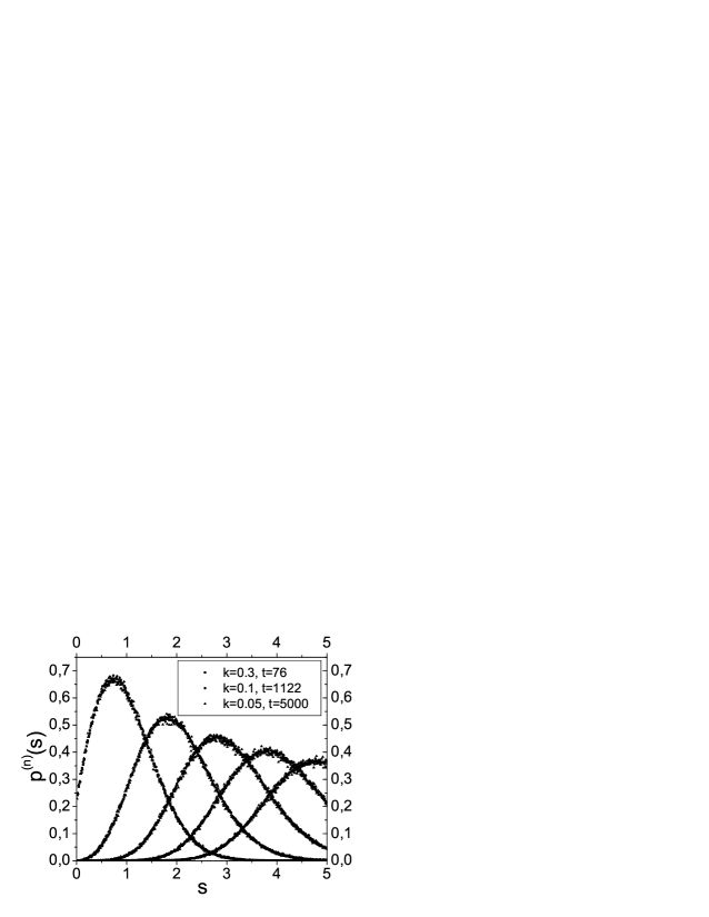
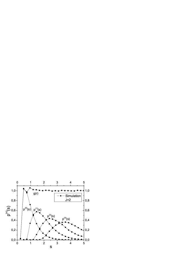
Equation (14) provides a good fit for the crossover in this reaction-diffusion model during its time evolution as we can see in figure 2. For the nearest neighbor distribution the fit is almost perfect for low and high values of , but for intermediate values we can see little differences in the interval for intermediate values of . In this figure all data was taken at different times with over realizations, the initial density was . The fit parameter is . We found the appropriate value of by using the numerical results for , equation (14) and the minimum square criteria 333This also can be done for values of near to or long times by using the numerical value of obtained from the simulation and taking into account that for the Berry-Robnik model..
The higher spacing distributions have been calculated with two methods. In the first one, we use our extension for the original Berry-Robnik Eq. (15) with equation (16). From now on, we call it the generalized Berry-Robnik (GBR) model. For the second one, we use equation (14) with the independent interval approximation (IIA). We call this method the Berry-Robnik+IIA (BR+IIA) model. In the IIA approximation, the entire statistical behavior of the system is described by the nearest neighbor distribution and the joint probability to find the particles in positions can be written as the product of independent product of the nearest neighbor distributions
| (33) |
where the partition function is the normalization constant
| (34) |
In the IIA approximation the correlations among intervals , , are neglected, for a review of this method see Ref. [5]. As is natural, the generalized Berry-Robnik model and the Berry-Robnik+IIA model are equivalents in the limit because in this regime those correlations are not strong and can be neglected.
In general, for the PCRW the fits are better for the GBR model than the BR+IIA. This means that for this system the information contained in is not enough to describe the entire statistical behavior of the system, i.e., the correlation among intervals can not be neglected as it happens in the BR+IIA model. These correlations can be neglected only for small times ), when the particles do not coalesce enough to build strong correlations between them. The value of as a function of can be computed from equation (30) as follows. Integrating Eq. (30), it is easy to find
| (35) |
Because of the reaction between particles, grows in time for making possible to write as plus an increment . In this way Eq. (35) takes the form
| (36) |
The correlations between particles can be neglected for small times when , then, we can neglect in Eq. (36). Finally if we consider that must be a fraction of , we find
| (37) |
This equation was derived first in Ref. [9]. From Eq. (37), it is clear that there is a time where the interaction between particles goes unnoticed even in the case of , where, is the typical time that one particle needs to reach one of its nearest neighbors. In the limit , we have as is natural because in this case is a constant.
We conclude, that, for the PCRW the spacing distribution and the pair correlation functions can be approximated from the uncorrelated superposition of a Poisson and a Wigner distribution functions as is proposed in the GBR model.
An alternate way to analyze the crossover of this system, is to study the spacing distribution functions at a fixed given time, but for different values of . In order to establish a connection between this picture for the transition and the one shown in figure 2, it is necessary to find the correct combination of and which gives the same statistical behavior for different values of these parameters. To find it, in figure 3-(a) we show the behavior of as a function of for different values of . We found that making the change of variable
| (38) |
all lines shown in figure 3-(a) collapse in a single one, see figure 3-(b). Then, different combinations of and with fixed give the same statistical behavior, i.e., give the same value for the fit parameter . This is shown in figure 4, the data was taken in all cases over realizations with . For large values of , , we found that and for low values of , , .
The physical meaning of the change of variable (38) is clear if we introduce the crossover time, , between the intermediate regime (which starts when ) and the long-time regime (when renormalizes to 1). This time is estimated in Ref. [9], by expanding Eq. (31) in powers of ,
| (39) |
which is precisely the scaling factor used in figure 3-(b). The change of variable (38) is .
4 Crossover in the quasi one dimensional gas system
This system was originally studied in [11]. There, the authors studied the biased diffusion of two species in a fully periodic rectangular lattice half filled with two types of particles labeled by their charge, there are particles with charge and particles with charge . An infinite external field drives the two species in opposite directions along the axis (long axis). The only interaction between particles is an excluded volume constraint, i.e., each lattice site can be occupied by only one particle. The system evolves in time according to the following dynamical rules:
-
1.
particles are randomly inserted in a rectangular lattice, particles and particles , the remaining sites are empty. Periodic boundary conditions are imposed in both directions of the lattice. Let the axis be the long axis of length .
-
2.
Two neighbor sites are chosen at random. The contents of the sites are exchanged with probability if the neighbor sites are particle-hole, but if they are particle-particle the contents are exchanged with probability . The exchanges which result in particles moving in the positive/negative direction are forbidden due to the action of the external field.
-
3.
A time unit, corresponds to attempts of exchange.
With these dynamical rules, this system evolves with formation of domains for low values of , see figure 5-(b) and 5-(c). In this regime, the average length of domains grows in time and while the size of the domains remains much smaller than the total size of the system, the domain size distribution exhibits a dynamic scaling. In the long time limit, the system reaches a non-equilibrium steady state (NESS) where there is only one macroscopic domain. The length of the macroscopic domain depends on , for example for it has an approximate size of . Additionally, for low values of , this macroscopic domain has not a simple charge distribution and it almost contains no holes. The macroscopic domain is not in equilibrium because there are particles (travelers) which leak out from one end of this domain and travel along the lattice until they reach the other end of this domain, see figure 5-(b). In the case of large values of the system remains homogeneous, i.e., disorganized without domain formation, as we can see in figure 5-(e). For intermediate values of , the macroscopic domain is not well formed, it has many holes and it is unstable. In this case there are many travelers and small length domains, see figure 5-(d).
In order to obtain quantitative results, we measure the length of a domain by using the coarse grained approximation (CG) defined in [11]. This approximation allows us to map the quasi one-dimensional lattice into a one-dimensional lattice. For any configuration on the lattice, we construct an effective one-dimensional one, with occupation numbers zero or one on a sites line, as follows. At each site , we assign if there are or less particles in the sites around it, including the -th column of the original lattice. We assign 1 otherwise, then, we assign in the -th site of the one-dimensional lattice if there are more particles than holes in the sites around the -th column in the original lattice 444In our description we take only four neighbor lines around the -th column, two at the left and two at the right. This election is arbitrary however the results are not so sensitive to it. If we take less neighbor lines we improve the measure of the small domains getting worse the measure of big domains and vice versa. Our choice of four neighbor lines allows us a reasonable measure of small and big domains.. In this simplified description a domain is a simple consecutive sequence of ones and its size is just the length of this string.
In figure 6, we show the behavior of for six values of . It is evident the NESS behavior in the long time limit when reaches its maximum value which depends on . Additionally, we found that in the NESS regime also depends on the size of the lattice for all values of , in fact for it is well know that . In figure 7, we show for and different values of . The value of increases with the value of and we can expect that it reaches its maximum value in the limit . We can conclude that for finite systems , in the NESS, depends on and .
For , we found in the scaling regime , this result coincides with the one found in [11]. For lower values of it seems that there is also a dynamical scaling region whose size decreases when increases. Naturally, for the systems remains homogeneous. Note that is very different for and cases, because for there are more travelers than in , see figure 5.

In figure 8, we show the spacing distribution and the pair correlation functions for the gas system for different values of . As it can be expected, the CG description is not appropriate to measure the length of small domains. However, this method allows us to measure of the length of big domains. For all values of , the nearest neighbor spacing distribution function is well fitted by Berry-Robnik model for high values of . For small values of , is well described by the Wigner distribution. In the case of , the nearest neighbor distribution is described by the Poisson distribution. However, the generalized Berry-Robnik model does not describe the next spacing distributions nor the pair correlation function with enough precision. The differences between the pure coalescing random walk (PCRW for ) and the gas system was already studied in Ref. [5] for the case of . There the authors found that the independent interval approximation (IIA) is a better model for the gas system than the CRW model. The results that we found for the Berry-Robnik+IIA model are shown in figure 8. We can see that the Berry-Robnik+IIA model is a better approximation for the statistical behavior of the gas for all values of . This fact suggests that, as it happens for , the domains in this system are not strongly correlated for all values of and because of that those correlations can be neglected.
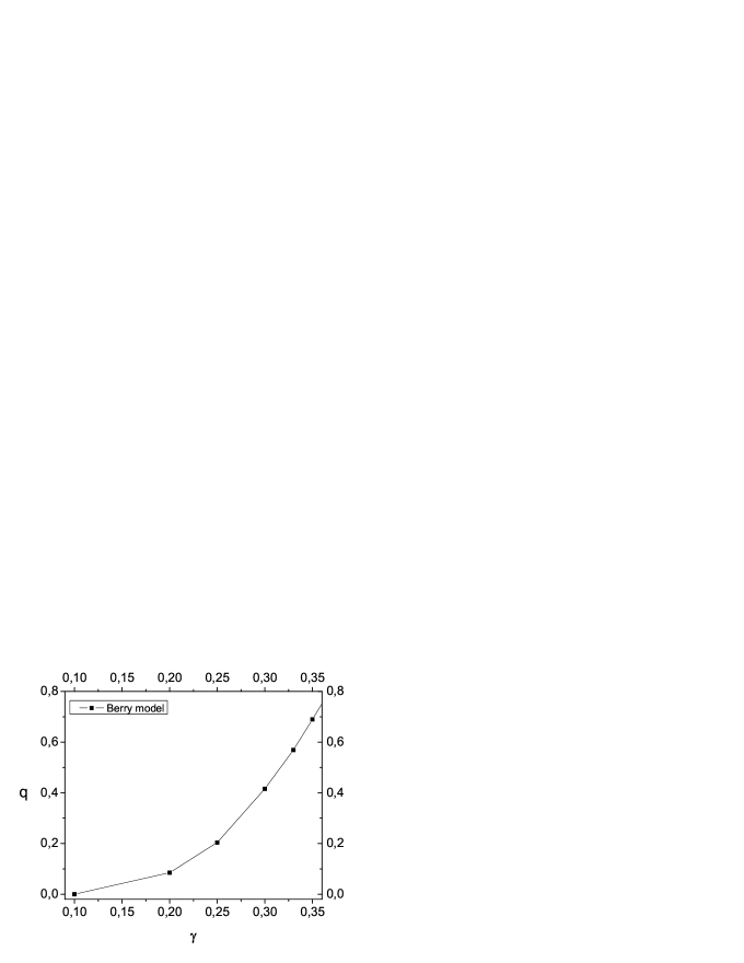
In figure 9, we show the behavior of as a function of in the interval . We found that at least for the system is in a disorganized state, i.e., its statistical behavior is well described by the Poisson distribution for large values of and fits give . In all fits used to find as function of we eliminated the regions where the points are highly dispersed, i.e., where the coarse grain method does not measure the length of domains with enough precision.
5 Crossover in the spin system
This system was originally introduced in Ref. [12]. There, the authors consider a lattice of length with spins up (“”) and spins down (“”) with . Periodic boundary conditions are imposed. The spin-flip events are:
-
1.
.
-
2.
.
-
3.
.
-
4.
.
The transition probability rate for a process from left to right is for and for . The constant is the nearest neighbor coupling between spins, is the energy associated to an external field which drives the up (“”) spins to the right and the down (“”) spins to the left, and the thermal energy (temperature times Boltzmann constant).
In Ref. [12] the authors restrict their study to the regime . In this regime the microscopic dynamics of the lattice of spins may be mapped into one for an array domain dynamics, which provides a good approximation in this regime, for more information see [5, 6, 8, 12, 13]. With this macroscopic description in Ref. [5] the authors show that this system has a statistical behavior very similar to the one of the gas system. Additionally, the system exhibits dynamical scaling behavior and, in the long time limit, the system reaches the NESS, where there are two macroscopic domains which move in opposite directions. However, this domain model does not allow us study the crossover of the system between organized and disorganized states because it is valid only in the regime . To study the crossover regime we must to use the microscopic dynamical rules listed above. In all simulations, we took and .
In figure 10-(b), we can see the asymptotic state for the spin system for large values of where there are only two stable macroscopic domains and . For , domain formation is not perceptible, see figure 10-(e) which it is almost identically to the disorganized initial state figure 10-(a). However, as we will see soon, the average length of domains is different in both cases. In the NESS, for low values of there is domain destruction and formation, in such way that is constant with a value lower than . As we can see in figure 11, for low values of , the statistical behavior of the spin system in the NESS is well described by the Poisson distribution. That means that the system remains in a disorganized state where the average length of domains is bigger than the initial one (). We can see slight differences near , this happens because we used in our simulation a discrete finite lattice.

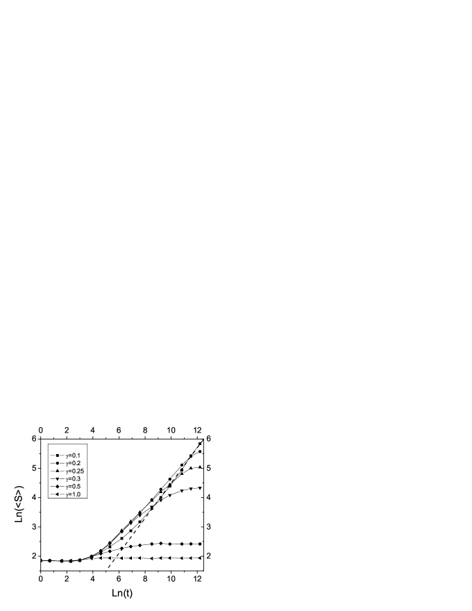
In figure 12, we can see the average length of domains as a function of time . In this case the behavior of is different from the one found in the PCRW and in the gas system. For large values of , the spin system reaches metastable states where is almost constant. Note that in all cases, the metastable state starts when the domain density is , i.e., when the system, in the statistical average sense, is filled with domains of the form . This is a consequence of the microscopical dynamical rules that we use, because they take into account interaction among four neighbors spins. For large enough values of , these domains have a low probability of destruction setting the system into a metastable state. In figure 13, we show the spacing distribution function in the metastable states, the level repulsion is present. After some time, starts to grow again in time. In the PCRW and in the gas systems the metastable states are not present. Once the metastable states ends, the domain formation in the system continues in such way that the average size of domains increases again. The length in time of these metastable states depends on the value of (with ). In fact for this region is absent but for bigger values of its size increases. Nevertheless, does not seem to depend on the length of the system in the scaling regime, it is the same for , the differences arises near to the NESS naturally 555The case was verified but is not included in the figure.. In figure 12, for , the system seems to reach another metastable state where for and for . For , the scaling region has a considerable size but this region for lower values of is smaller. From figure 12 it is evident that the value of in the NESS regime depends on the size of the system, as it also happens in the gas system. In the inset of figure 12, we compare for and , in the last case there is domain formation and it seems that only for there is not domain formation.
As it happens in the gas system, the statistical behavior of this model is better described by the Berry-Robnik+IIA than the generalized Berry-Robnik model. In figure 14, we show the statistical behavior of the system for different values of . For , the system evolves in time remaining disorganized, as we expected. However, we cannot compare directly its spacing distributions with our analytical model because of the effects of the discrete finite lattice that we use in our simulations. In fact, as we can see in figure 14, instead of as it is predicted by the continuous Poisson distribution. This result can be understood if we remember that, in a lattice, the lowest value for which the nearest spacing distribution is defined, is , with the density of particles. In our case, for in each spin species. This technical problem is usually solved taking low density values as we did it in the PCRW, where we took . However, we cannot do that in the spin system. We have to take small lattices because the simulation is very intensive and low densities give us a poor statistic. This is only a technical problem and we can be sure that in the limit of low densities and small values of , the system is well described by the continuous Poisson distribution. To corroborate this, we compare the results of our simulation for with the discrete version of the Poisson distribution (, , etc.).
For the system sets into an organized state where there is domain formation. In this case, is well fitted by the Wigner distribution. For , the results of our microscopic simulation coincides with the results of the macroscopic array domains simulation in the regime . For intermediate values, the system shows a mixed state. If we do not take into account the discrete finite lattice, for all values of , is well described by the Berry-Robnik+IIA model. This suggest that for this system the correlation between domains are not strong as it happen in the gas system. For low densities and values of near 1, we expect that the generalized Berry-Robnik and the Berry-Robnik+IIA models are a good approximation for higher spacing distribution functions () and for the pair correlation function because in this regime the correlation between domains can be neglected.
In our numerical simulations we took and realizations. The measures were taken at different times using two lattices: and , in order to confirm the scaling property. For , we took and for and . For , we took for and for . For , we took for and for . For , the system remains disorganized and the time when the data is taken is irrelevant.
6 Conclusion
In all systems considered in this paper, the original Berry-Robnik model gives us a good fit for the nearest neighbor distribution , i.e., can be approximated by the uncorrelated superposition of one Wigner and one Poisson distribution functions. The biggest differences in the fits are given when the densities of both sequences have similar values. We calculate the next spacing distribution functions by using two methods, the GBR and the BR+IIA. We found that the GBR model gives us a good approximation for the statistical behavior of the PCRW and the BR+IIA model is a good approximation for the gas and spin systems. This fact suggest that the correlation between domains in the gas and spin system are not strong and can be neglected in a first approximation but in the PCRW the correlations between particles cannot be neglected.
Our analytical models are simple and allow us to have a quantitative measure of the degree of order/disorder of the systems through the parameter . For the system is completely disordered and is described by the Poisson distribution, that means that the system is homogeneous, in the statistical average sense. For the system is organized and is described by the Wigner distribution. In the particular case of the PCRW implies that there is an effective repulsion between particles and in the case of the gas and spin systems means domain formation. Unfortunately, the information about the interaction between particles/domains cannot be extracted easily from the statistical behavior in non-equilibrium systems. However, by using the BR+IIA model it is possible to calculate in an approximate way the interaction potential between domain borders for the gas and spin systems, as follows. Comparing (33) with a Boltzmann factor with an inverse temperature , is straightforward to show that, under the BR+IIA approximation, the statistics of the domain borders is approximately equivalent to a system with particles which interact according to the potential
| (40) |
where
| (41) |
and . Thus, the statistics of the domain edges of the gas and spin systems in their crossover regimes is approximately equivalent to a statistical equilibrium system of particles on a circle interacting through the nearest neighbor pair potential (40). Note that for , Eq. (40) reduces to
| (42) |
as we can expect from Ref. [5]. Naturally, for the interaction potential is a constant and the interaction force between domain edges vanishes.
In the crossover between order and disorder all systems lose their level repulsion properties, i.e., the correlations between domains/particles decrease. In the PCRW, the correlations between particles arises from the coalescence reaction for , in the gas case, correlations arise from the mutual obstruction of particles for . For the spin system, taking and , the crossover depends only on and the correlations arise for .
The gas and spin systems have a similar statistical behavior in the crossover between organized and disorganized states but is very different in both cases. The metastable regions that we found in the spin system are not present in the gas system nor in the PCRW. In fact metastable regions are not predicted by the macroscopic dynamical rules used in Ref. [12]. In the PCRW there is a time where the interaction goes unnoticed which depends on the parameter . In the gas an spin systems it seems that this time does not depend on the parameters and respectively.
Finally, for the PCRW, we found that the parameter , which characterize the crossover, can be scaled in a function of a single argument by making the change of variable . The scaling factor is proportional to the crossover time between intermediate regime and long time regime, .
Acknowledgments
The authors thank F. van Wijland for valuable comments and observations. This work was partially supported by an ECOS Nord/COLCIENCIAS action of French and Colombian cooperation and by Comité de Investigaciones y Posgrados, Facultad de Ciencias, Universidad de los Andes.
References
- [1] M. V. Berry and M. Robnik, Semiclassical level spacings when regular and chaotic orbits coexist, J. Phys. A: Math. Gen. 17, 2413–2421 (1984).
- [2] P. Jacquod and J. P. Amiet, Evidence for the validity of the Berry-Robnik surmise in a periodically pulsed spin system, J. Phys. A: Math. Gen. 28, 4799–4811 (1995).
- [3] V. Lopac, S. Brant and V. Paar, Level density fluctuations and characterization of chaos in the realistic model spectra for odd-odd nuclei, Z. Phys. A. 356, 113–118 (1996).
- [4] D. ben-Avraham and S. Havlin. Diffusion and reactions in fractals and disordered systems, Cambridge University Press (2000).
- [5] D. L. González and G. Téllez, Statistical behavior of domain systems, Phys. Rev. E 76, 011126 (2007).
- [6] D. L. González and G. Téllez, Is The Nearest Neighbor Distribution Enough to Describe The Statistical Behavior Of A Domain System?, To be published in the Traffic granular flow 2007.
- [7] D. ben-Avraham and É. Brunet, On the relation between one-species diffusion-limited coalescence and annihilation in one dimension, J. Phys. A: Math. Gen. 38, 3247–3252 (2005).
- [8] D. L. González and G. Téllez, Wigner domains for domain systems, J. Stat. Phys. 132, 187–205 (2008).
- [9] D. Zhong and D. Ben-Avraham. Diffusion-limited coalescence with finite reaction rates in one dimension. J. Phys. A: Math. Gen. 28 33–44 (1995).
- [10] V. Privman and C. R. Doering, Crossover from rate-equation to diffusion-controlled kinetics in two particle coagulation, Phys. Rev. E 48, 846–851 (1993).
- [11] J. Mettetal, B. Schmittmann and R. Zia, Coarsening dynamics of a quasi one-dimensional driven lattice gas, Europhysics Lett. 58, 653–659 (2002).
- [12] S. J. Cornell and A. J. Bray, Domain growth in a one-dimensional driven diffusive system, Phys. Rev. E 54, 1153–1160 (1996).
- [13] V. Spirin, P. L. Krapivsky and S. Redner, Coarsening in a driven Ising chain with conserved dynamics, Phys. Rev. E 60, 2670–2676 (1999).
- [14] P. A. Alemany and D. ben-Avraham, Inter-particle distribution functions for one-species diffusion-limited annihilation, , Phys. Lett. A. 206, 18–25 (1995).
- [15] B. Derrida, V. Hakim and R. Zeitak, Persistent spins in the linear diffusion approximation of phase ordering and zeros of stationary gaussian processes, Phys. Rev. Lett. 77, 2871–2874 (1996).
- [16] S. N. Majumdar, C. Sire, A. J. Bray and S. J. Cornell, Nontrivial exponent for simple diffusion, Phys. Rev. Lett. 77, 2867–2870 (1996).
- [17] P. L. Krapivsky and E. Ben-Naim, Domain statistics in coarsening systems, Phys. Rev. E 56, 3788–3798 (1997).
- [18] E. Ben-Naim and P. L. Krapivsky, Domain number distribution in the nonequilibrium Ising model, J. Stat. Phys. 93, 583–601 (1998).
- [19] Z. W. Salsburg, R. W. Zwanzig and J. G. Kirkwood, Molecular distribution functions in a one-dimensional fluid, J. Chem. Phys. 21, 1098–1107 (1953).