Monte Carlo analysis of CLAS data

Abstract

We present a fit of the virtual-photon scattering asymmetry of polarized Deep Inelastic Scattering which combines a Monte Carlo technique with the use of a redundant parametrization based on Neural Networks. We apply the result to the analysis of CLAS data on a polarized proton target.

1 Introduction

In High Energy Physics assessing the uncertainty of a function (i. e., a probability measure on a space of functions) from a finite set of experimental data points has become a subject of great interest in the last years. The case of structure functions in polarized Deep Inelastic Scattering (DIS) is interesting in this respect, because it provides a good testing ground for the fitting technique on a relatively small set of data.

In our analysis we have used the data for the virtual-photon scattering asymmetry $A_{1}(x,Q^{2})$, since in this case the theoretical assumptions are minimized, and then different settings for the reconstruction of $g_{1}(x,Q^{2})$ can be tested separately. Indeed, the extraction of the polarized structure function $g_{1}(x,Q^{2})$ from the experimental measured asymmetries $A_{\parallel}$ and $A_{\perp}$ is not so trivial: assumptions have to be made (say, the choice of a parametrization for the unpolarized structure function) and different experimental collaborations sometimes quote different results. Once a fit of $A_{1}(x,Q^{2})$ is provided, such a parametrization might be an ideal input for a fit based on factorization scheme-invariant evolution equations aiming to a precise determination of $\alpha_{s}$, as proposed in [2, 3].

In [4] we have adopted the technique presented in [5, 6, 7] to the available data for polarized DIS. Here we present some details of our analysis not included in [4], as an example of application of our results.

2 The technique

The first step is the propagation of experimental information from the finite set of data points to the parametrization. Since experimental data are occurrences of a probability distribution, we use a Monte Carlo technique to sample such a distribution. This sampling is performed by generating $N_{rep}$ artificial replicas of data following a multi-gaussian distribution centered on each data point with the variance given by the experimental error

$$A_{1}^{(art),k}(x,Q^{2})=\left(1+r_{k,N}\sigma_{N}\right)\left(A_{1}^{(exp)}(x,Q^{2})+r_{k,t}\sigma_{t}(x,Q^{2})\right)\,,$$ (1)

where $r$ are Gaussian distributed random numbers, $\sigma_{t}$ is is the total uncorrelated error, obtained by summing in quadrature the statistical and uncorrelated systematic errors, $\sigma_{N}$ is the normalization multiplicative error. At this stage of the analysis we neglect correlated systematic errors since they are not available for all the experiments considered. Moreover the measurement of polarized structure functions is dominated by statistical errors.

The number of Monte Carlo replicas of the data is determined by the requirement that the average over the replicas reproduces the features (central values and errors) of the original experimental data with a given accuracy. In practice here we use $N_{rep}=100$.

The second step is to build a representation of the probability measure in the space of asymmetry functions. This construction can be done by taking a given functional form, and determining its parameters by fitting each of the generated replicas. In order to minimize the bias due to the assumptions made on the shape of the fitted functions we make use of a redundant parametrization, that is a parametrization with a sufficiently large number of parameters so that not only the underlying physical law, but also the statistical fluctuations of the data could be reproduced. Of course within this framework over-fitting is allowed and the minimization becomes crucial. In practise we use a Neural Network which has 20 tunable parameters to perform a fit to 100 data points and we stop the minimization, when we start fitting statistical noise (see [4] for details).

At the end of this procedure any observable can be computed from the fit by averaging over the sample. As an example, if we neglect the contribution of $g_{2}(x,Q^{2})$, we have

$$g_{1}(x,Q^{2})\simeq\frac{1}{N_{rep}}\sum_{k=1}^{N_{rep}}A_{1}^{(fit),k}(x,Q^{2})F_{1}(x,Q^{2})\,.$$ (2)

3 Results

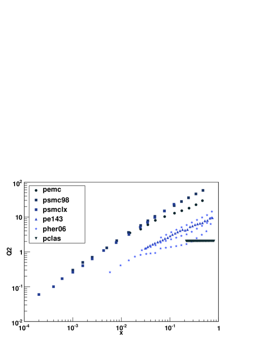
As an application and a test of our result, we compare our extraction of $g_{1}(x,Q^{2})$ to CLAS data [8], which have not been used in the fit. In Figure 1 we show the kinematic range spanned by the data used in the fit (see also Table 1) together with the bin of CLAS data against which we want to check our parametrisation. As it can be easily seen most of the CLAS data are in a region where our fit is asked to extrapolate, both in $x$ and in $Q^{2}$.

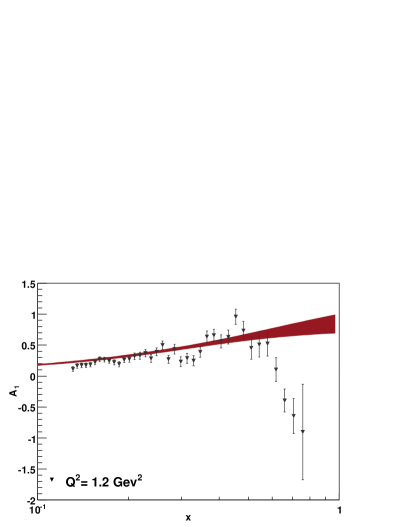
Comparing our extraction of $A_{1}(x,Q^{2})$ with data (see Figure 2 left pad), we notice that our description and CLAS data are compatible within 2-$\sigma$ error band, and that resonances are naturally averaged by the fit.

Proton	$x$ range	$Q^{2}(GeV^{2})$ range	$N_{dat}$
EMC	0.0150 - 0.466	3.50 - 29.5	10
SMC	0.0010 - 0.480	0.30 - 58.0	15
SMC low-$x$	0.0001 - 0.121	0.02 - 23.1	15
E143	0.0310 - 0.75	1.27 - 9.52	28
HERMES06	0.0058 - 0.7311	0.26 - 14.29	45

Table 1: General features of experimental data used in the fit

In order to obtain the polarized structure function $g_{1}(x,Q^{2})$, we have to supplement our parametrization with some assumptions, whose impact can be tested easily once a parametrization of $A_{1}(x,Q^{2})$ is given. In the present analysis we take $g_{2}(x,Q^{2})=g_{2}^{WW}(x,Q^{2})$, and

$$F_{1}(x,Q^{2})=\frac{1+\gamma^{2}}{2x\,(1+R(x,Q^{2}))}F_{2}(x,Q^{2})\,$$ (3)

where $\gamma^{2}=4xM^{2}/Q^{2}$, $R(x,Q^{2})$ is given from the SLAC parametrization [9, 10], and $F_{2}(x,Q^{2})$ from [6]. We have

$$g_{1}(x,Q^{2})=\frac{1+\gamma^{2}}{2x\,(1+R(x,Q^{2}))}\frac{1}{N_{rep}}\sum_{k=1}^{N_{rep}}\left[A_{1}^{(fit),k}(x,Q^{2})F_{2}^{k}(x,Q^{2})+\gamma^{2}g_{2}^{k}(x,Q^{2})\right]\,,$$ (4)

with

$$g_{2}^{k}(x,Q^{2})=-g_{1}^{k}(x,Q^{2})+\int_{x}^{1}\frac{dy}{y}\,g_{1}^{k}(x,Q^{2})\,.$$ (5)

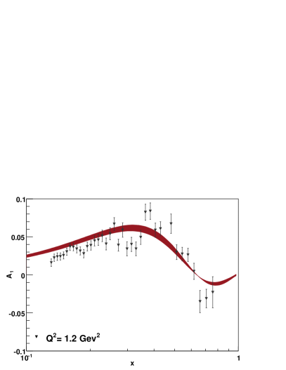
Equations (4) and (5) explicitly show how to evaluate any quantity depending on the asymmetry, together with its associated error, in a straightforward way. The result shown in the right pad of Figure 2 is consistent with the one given in [11].

Figure 1: Kinematics of the experimental data used in the analysis plus the CLAS bin used to test our fit.

Figure 2: The fitted asymmetry $A_{1}(x,Q^{2})$ and reconstruction of $g_{1}(x,Q^{2})$ compared to CLAS data not used in the fit

We have presented a fit based on a large fraction of the available experimental data for the asymmetry $A_{1}(x,Q^{2})$, and we have applied this result to predict some of the remaining data that were not included in the fit and lie in a region where our asymmetry needs to be extrapolated. We find the result of this comparison to be satisfactory. We conclude that our parametrization provides an interesting tool to study quark-hadron duality since no QCD evolution is used and averages of the structure function over resonances are naturally guaranteed by the smoothness of the fit (see [11] and references therein for further details on a usual approach to quark-hadron duality).

4 Acknowledgments

LDD is supported by an STFC advanced fellowship.