2 Solutions of Einstein-Maxwell-dilaton equations
The action of 5D EMd gravity is given by
S = 1 16 π ∫ d 5 x − g ( R − 8 3 g μ ν ∂ μ Φ ∂ ν Φ − 1 2 e − 4 3 α Φ F μ ν F μ ν ) , 𝑆 1 16 𝜋 superscript 𝑑 5 𝑥 𝑔 𝑅 8 3 superscript 𝑔 𝜇 𝜈 subscript 𝜇 Φ subscript 𝜈 Φ 1 2 superscript 𝑒 4 3 𝛼 Φ subscript 𝐹 𝜇 𝜈 superscript 𝐹 𝜇 𝜈 \displaystyle S=\frac{1}{16\pi}\int d^{5}x\sqrt{-g}\left(R-\frac{8}{3}g^{\mu\nu}\partial_{\mu}\Phi\partial_{\nu}\Phi-\frac{1}{2}e^{-\frac{4}{3}\alpha\Phi}F_{\mu\nu}F^{\mu\nu}\right), (1)
and metric we consider is given by
d s 2 = f ( d ρ 2 + d z 2 ) + g a b d x a d x b , ( a , b = 0 , 1 , 2 ) \displaystyle ds^{2}=f(d\rho^{2}+dz^{2})+g_{ab}dx^{a}dx^{b},\quad(a,b=0,1,2) (2)
where f 𝑓 f g a b subscript 𝑔 𝑎 𝑏 g_{ab} ρ 𝜌 \rho z 𝑧 z
R μ = ν 4 3 ∂ μ Φ ∂ ν Φ + 2 e − 4 3 α Φ ( F μ σ F ν σ − 1 6 δ μ F β σ ν F β σ ) , \displaystyle R^{\mu}{}_{\nu}=\frac{4}{3}\partial^{\mu}\Phi\partial_{\nu}\Phi+2e^{-\frac{4}{3}\alpha\Phi}\left(F^{\mu\sigma}F_{\nu\sigma}-\frac{1}{6}\delta^{\mu}{}_{\nu}F^{\beta\sigma}F_{\beta\sigma}\right), (3)
∇ 2 Φ = − α 2 e − 4 3 α Φ F β σ F β σ , superscript ∇ 2 Φ 𝛼 2 superscript 𝑒 4 3 𝛼 Φ subscript 𝐹 𝛽 𝜎 superscript 𝐹 𝛽 𝜎 \displaystyle\nabla^{2}\Phi=-\frac{\alpha}{2}e^{-\frac{4}{3}\alpha\Phi}F_{\beta\sigma}F^{\beta\sigma}, (4)
( e − 4 3 α Φ F μ ν ) ; μ = 0 , \displaystyle(e^{-\frac{4}{3}\alpha\Phi}F^{\mu\nu}{})_{;\mu}=0, (5)
with
F μ ν = A ν , μ − A μ , ν . \displaystyle F_{\mu\nu}=A_{\nu},_{\mu}-A_{\mu},_{\nu}. (6)
Here α 𝛼 \alpha det g = − ρ 2 𝑔 superscript 𝜌 2 \det g=-\rho^{2} g = ( g a b ) 𝑔 subscript 𝑔 𝑎 𝑏 g=(g_{ab}) U ( 1 ) 𝑈 1 U(1)
g = diag ( − h 1 − 1 h 2 − 1 , [ ρ 2 + z 2 − z ] h 1 , [ ρ 2 + z 2 + z ] h 2 ) , 𝑔 diag superscript subscript ℎ 1 1 superscript subscript ℎ 2 1 delimited-[] superscript 𝜌 2 superscript 𝑧 2 𝑧 subscript ℎ 1 delimited-[] superscript 𝜌 2 superscript 𝑧 2 𝑧 subscript ℎ 2 \displaystyle g={\rm diag}\left(-h_{1}^{-1}h_{2}^{-1},\left[\sqrt{\rho^{2}+z^{2}}-z\right]h_{1},\left[\sqrt{\rho^{2}+z^{2}}+z\right]h_{2}\right), (7)
A 0 = − χ , A 1 = A 2 = A ρ = A z = 0 , formulae-sequence subscript 𝐴 0 𝜒 subscript 𝐴 1 subscript 𝐴 2 subscript 𝐴 𝜌 subscript 𝐴 𝑧 0 \displaystyle A_{0}=-\chi,\quad A_{1}=A_{2}=A_{\rho}=A_{z}=0, (8)
where h 1 subscript ℎ 1 h_{1} h 2 subscript ℎ 2 h_{2} ρ 𝜌 \rho z 𝑧 z χ ( ρ , z ) 𝜒 𝜌 𝑧 \chi(\rho,z)
[ ρ ( ln h i ) , ρ ] , ρ + [ ρ ( ln h i ) , z ] , z = − 4 ρ 3 h 1 h 2 e − 4 3 α Φ ( χ , ρ 2 + χ , z 2 ) , ( i = 1 , 2 ) \displaystyle[\rho(\ln h_{i}),_{\rho}],_{\rho}+[\rho(\ln h_{i}),_{z}],_{z}=-\frac{4\rho}{3}h_{1}h_{2}e^{-\frac{4}{3}\alpha\Phi}(\chi,_{\rho}^{2}+\chi,_{z}^{2}),\quad(i=1,2) (9)
( ln f ) , ρ + ρ ρ 2 + z 2 − 1 2 ( ρ ρ 2 + z 2 [ ( ln h 1 ) , z − ( ln h 2 ) , z ] \displaystyle(\ln f),_{\rho}+\frac{\rho}{\rho^{2}+z^{2}}-\frac{1}{2}\Biggr{(}\frac{\rho}{\sqrt{\rho^{2}+z^{2}}}[(\ln h_{1}),_{z}-(\ln h_{2}),_{z}] (10)
+ ρ 2 + z 2 + z ρ 2 + z 2 ( ln h 1 ) , ρ + ρ 2 + z 2 − z ρ 2 + z 2 ( ln h 2 ) , ρ \displaystyle+\frac{\sqrt{\rho^{2}+z^{2}}+z}{\sqrt{\rho^{2}+z^{2}}}(\ln h_{1}),_{\rho}+\frac{\sqrt{\rho^{2}+z^{2}}-z}{\sqrt{\rho^{2}+z^{2}}}(\ln h_{2}),_{\rho} (11)
+ ρ [ ( ln h 1 ) , ρ 2 + ( ln h 2 ) , ρ 2 + ( ln h 1 ) , ρ ( ln h 2 ) , ρ ] \displaystyle+\rho[(\ln h_{1}),_{\rho}^{2}+(\ln h_{2}),_{\rho}^{2}+(\ln h_{1}),_{\rho}(\ln h_{2}),_{\rho}] (12)
− ρ [ ( ln h 1 ) , z 2 + ( ln h 2 ) , z 2 + ( ln h 1 ) , z ( ln h 2 ) , z ] ) \displaystyle-\rho[(\ln h_{1}),_{z}^{2}+(\ln h_{2}),_{z}^{2}+(\ln h_{1}),_{z}(\ln h_{2}),_{z}]\Biggr{)} (13)
= − 2 ρ [ h 1 h 2 e − 4 3 α Φ ( χ , ρ 2 − χ , z 2 ) − 2 3 ( Φ , ρ 2 − Φ , z 2 ) ] , \displaystyle=-2\rho\left[h_{1}h_{2}e^{-\frac{4}{3}\alpha\Phi}(\chi,_{\rho}^{2}-\chi,_{z}^{2})-\frac{2}{3}(\Phi,_{\rho}^{2}-\Phi,_{z}^{2})\right], (14)
( ln f ) , z + z ρ 2 + z 2 − 1 2 ( − ρ ρ 2 + z 2 [ ( ln h 1 ) , ρ − ( ln h 2 ) , ρ ] \displaystyle(\ln f),_{z}+\frac{z}{\rho^{2}+z^{2}}-\frac{1}{2}\Biggr{(}-\frac{\rho}{\sqrt{\rho^{2}+z^{2}}}[(\ln h_{1}),_{\rho}-(\ln h_{2}),_{\rho}] (15)
+ ρ 2 + z 2 + z ρ 2 + z 2 ( ln h 1 ) , z + ρ 2 + z 2 − z ρ 2 + z 2 ( ln h 2 ) , z \displaystyle+\frac{\sqrt{\rho^{2}+z^{2}}+z}{\sqrt{\rho^{2}+z^{2}}}(\ln h_{1}),_{z}+\frac{\sqrt{\rho^{2}+z^{2}}-z}{\sqrt{\rho^{2}+z^{2}}}(\ln h_{2}),_{z} (16)
+ 2 ρ [ ( ln h 1 ) , ρ ( ln h 1 ) , z + ( ln h 2 ) , ρ ( ln h 2 ) , z ] \displaystyle+2\rho[(\ln h_{1}),_{\rho}(\ln h_{1}),_{z}+(\ln h_{2}),_{\rho}(\ln h_{2}),_{z}] (17)
+ ρ [ ( ln h 1 ) , ρ ( ln h 2 ) , z + ( ln h 1 ) , z ( ln h 2 ) , ρ ] ) \displaystyle+\rho[(\ln h_{1}),_{\rho}(\ln h_{2}),_{z}+(\ln h_{1}),_{z}(\ln h_{2}),_{\rho}]\Biggr{)} (18)
= − 4 ρ ( h 1 h 2 e − 4 3 α Φ χ , ρ χ , z − 2 3 Φ , ρ Φ , z ) , \displaystyle=-4\rho\left(h_{1}h_{2}e^{-\frac{4}{3}\alpha\Phi}\chi,_{\rho}\chi,_{z}-\frac{2}{3}\Phi,_{\rho}\Phi,_{z}\right), (19)
( ρ h 1 h 2 χ , ρ ) , ρ + ( ρ h 1 h 2 χ , z ) , z = 4 ρ 3 α h 1 h 2 ( Φ , ρ χ , ρ + Φ , z χ , z ) , \displaystyle(\rho h_{1}h_{2}\chi,_{\rho}),_{\rho}+(\rho h_{1}h_{2}\chi,_{z}),_{z}=\frac{4\rho}{3}\alpha h_{1}h_{2}(\Phi,_{\rho}\chi,_{\rho}+\Phi,_{z}\chi,_{z}), (20)
∇ 2 Φ = α h 1 h 2 e − 4 3 α Φ ( χ , ρ 2 + χ , z 2 ) , \displaystyle\nabla^{2}\Phi=\alpha h_{1}h_{2}e^{-\frac{4}{3}\alpha\Phi}({\chi},_{\rho}^{2}+\chi,_{z}^{2}), (21)
where ∇ 2 = ∂ ρ 2 + ∂ ρ / ρ + ∂ z 2 superscript ∇ 2 superscript subscript 𝜌 2 subscript 𝜌 𝜌 superscript subscript 𝑧 2 \nabla^{2}=\partial_{\rho}^{2}+\partial_{\rho}/\rho+\partial_{z}^{2} 9 20 21 h i subscript ℎ 𝑖 h_{i} Φ Φ \Phi χ 𝜒 \chi 14 19 f 𝑓 f
Note that Eq. (9
∇ 2 ( ln h i ) = − 4 3 h 1 h 2 e − 4 3 α Φ ( χ , ρ 2 + χ , z 2 ) . ( i = 1 , 2 ) \displaystyle\nabla^{2}(\ln h_{i})=-\frac{4}{3}h_{1}h_{2}e^{-\frac{4}{3}\alpha\Phi}(\chi,_{\rho}^{2}+\chi,_{z}^{2}).\quad(i=1,2) (22)
Then, combining these equations with Eq. (21
∇ 2 ( ln h i + 2 α 3 Φ ) superscript ∇ 2 subscript ℎ 𝑖 2 𝛼 3 Φ \displaystyle\nabla^{2}(\ln h_{i}+\frac{2\alpha}{3}\Phi) = \displaystyle= 2 3 ( α 2 − 2 ) h 1 h 2 e − 4 3 α Φ ( χ , ρ 2 + χ , z 2 ) , ( i = 1 , 2 ) \displaystyle\frac{2}{3}(\alpha^{2}-2)h_{1}h_{2}e^{-\frac{4}{3}\alpha\Phi}(\chi,_{\rho}^{2}+\chi,_{z}^{2}),\quad(i=1,2) (23)
∇ 2 ( ln h i − 2 α 3 Φ ) superscript ∇ 2 subscript ℎ 𝑖 2 𝛼 3 Φ \displaystyle\nabla^{2}(\ln h_{i}-\frac{2\alpha}{3}\Phi) = \displaystyle= − 2 3 ( α 2 + 2 ) h 1 h 2 e − 4 3 α Φ ( χ , ρ 2 + χ , z 2 ) . ( i = 1 , 2 ) \displaystyle-\frac{2}{3}(\alpha^{2}+2)h_{1}h_{2}e^{-\frac{4}{3}\alpha\Phi}(\chi,_{\rho}^{2}+\chi,_{z}^{2}).\quad(i=1,2) (24)
By defining H i subscript 𝐻 𝑖 H_{i} H ¯ i subscript ¯ 𝐻 𝑖 \bar{H}_{i}
H i = h i e 2 α 3 Φ , H ¯ i = h i e − 2 α 3 Φ , ( i = 1 , 2 ) formulae-sequence subscript 𝐻 𝑖 subscript ℎ 𝑖 superscript 𝑒 2 𝛼 3 Φ subscript ¯ 𝐻 𝑖 subscript ℎ 𝑖 superscript 𝑒 2 𝛼 3 Φ 𝑖 1 2
\displaystyle H_{i}=h_{i}e^{\frac{2\alpha}{3}\Phi},~{}\bar{H}_{i}=h_{i}e^{-\frac{2\alpha}{3}\Phi},~{}(i=1,2) (25)
these equations are rewritten as
∇ 2 ln H i superscript ∇ 2 subscript 𝐻 𝑖 \displaystyle\nabla^{2}\ln H_{i} = \displaystyle= 2 3 ( α 2 − 2 ) H ¯ 1 H ¯ 2 ( χ , ρ 2 + χ , z 2 ) , ( i = 1 , 2 ) \displaystyle\frac{2}{3}(\alpha^{2}-2)\bar{H}_{1}\bar{H}_{2}(\chi,_{\rho}^{2}+\chi,_{z}^{2}),\quad(i=1,2) (26)
∇ 2 ln H ¯ i superscript ∇ 2 subscript ¯ 𝐻 𝑖 \displaystyle\nabla^{2}\ln\bar{H}_{i} = \displaystyle= − 2 3 ( α 2 + 2 ) H ¯ 1 H ¯ 2 ( χ , ρ 2 + χ , z 2 ) , ( i = 1 , 2 ) \displaystyle-\frac{2}{3}(\alpha^{2}+2)\bar{H}_{1}\bar{H}_{2}(\chi,_{\rho}^{2}+\chi,_{z}^{2}),\quad(i=1,2) (27)
and Eq. (20
( ρ H ¯ 1 H ¯ 2 χ , ρ ) , ρ + ( ρ H ¯ 1 H ¯ 2 χ , z ) , z = 0 . \displaystyle(\rho\bar{H}_{1}\bar{H}_{2}\chi,_{\rho}),_{\rho}+(\rho\bar{H}_{1}\bar{H}_{2}\chi,_{z}),_{z}=0. (28)
From Eq. (25
H 1 H 2 = H ¯ 1 H ¯ 2 = h 1 h 2 , subscript 𝐻 1 subscript 𝐻 2 subscript ¯ 𝐻 1 subscript ¯ 𝐻 2 subscript ℎ 1 subscript ℎ 2 \displaystyle\frac{H_{1}}{H_{2}}=\frac{\bar{H}_{1}}{\bar{H}_{2}}=\frac{h_{1}}{h_{2}}, (29)
and the equations in Eq. (25
Φ Φ \displaystyle\Phi = \displaystyle= 3 4 α ( ln H i − ln H ¯ i ) , ( i = 1 , 2 ) 3 4 𝛼 subscript 𝐻 𝑖 subscript ¯ 𝐻 𝑖 𝑖 1 2
\displaystyle\frac{3}{4\alpha}(\ln H_{i}-\ln\bar{H}_{i}),\quad(i=1,2) (30)
ln h i subscript ℎ 𝑖 \displaystyle\ln h_{i} = \displaystyle= 1 2 ( ln H i + ln H ¯ i ) . ( i = 1 , 2 ) \displaystyle\frac{1}{2}(\ln H_{i}+\ln\bar{H}_{i}).\quad(i=1,2) (31)
By using these expressions, Eqs. (14 19
( ln f ) , ρ + ρ ρ 2 + z 2 − 1 4 ( ρ ρ 2 + z 2 [ ( ln H 1 ) , z − ( ln H 2 ) , z ] \displaystyle(\ln f),_{\rho}+\frac{\rho}{\rho^{2}+z^{2}}-\frac{1}{4}\Biggr{(}\frac{\rho}{\sqrt{\rho^{2}+z^{2}}}[(\ln H_{1}),_{z}-(\ln H_{2}),_{z}] (32)
+ ρ 2 + z 2 + z ρ 2 + z 2 ( ln H 1 ) , ρ + ρ 2 + z 2 − z ρ 2 + z 2 ( ln H 2 ) , ρ \displaystyle+\frac{\sqrt{\rho^{2}+z^{2}}+z}{\sqrt{\rho^{2}+z^{2}}}(\ln H_{1}),_{\rho}+\frac{\sqrt{\rho^{2}+z^{2}}-z}{\sqrt{\rho^{2}+z^{2}}}(\ln H_{2}),_{\rho} (33)
+ α 2 + 2 2 α 2 ρ [ ( ln H 1 ) , ρ 2 + ( ln H 2 ) , ρ 2 + ( ln H 1 ) , ρ ( ln H 2 ) , ρ \displaystyle+\frac{\alpha^{2}+2}{2\alpha^{2}}\rho\left[(\ln H_{1}),_{\rho}^{2}+(\ln H_{2}),_{\rho}^{2}+(\ln H_{1}),_{\rho}(\ln H_{2}),_{\rho}\right. (34)
− ( ln H 1 ) , z 2 − ( ln H 2 ) , z 2 − ( ln H 1 ) , z ( ln H 2 ) , z ] ) \displaystyle\left.-(\ln H_{1}),_{z}^{2}-(\ln H_{2}),_{z}^{2}-(\ln H_{1}),_{z}(\ln H_{2}),_{z}\right]\Biggr{)} (35)
− 1 4 ( ρ ρ 2 + z 2 [ ( ln H ¯ 1 ) , z − ( ln H ¯ 2 ) , z ] \displaystyle-\frac{1}{4}\Biggr{(}\frac{\rho}{\sqrt{\rho^{2}+z^{2}}}[(\ln\bar{H}_{1}),_{z}-(\ln\bar{H}_{2}),_{z}] (36)
+ ρ 2 + z 2 + z ρ 2 + z 2 ( ln H ¯ 1 ) , ρ + ρ 2 + z 2 − z ρ 2 + z 2 ( ln H ¯ 2 ) , ρ \displaystyle+\frac{\sqrt{\rho^{2}+z^{2}}+z}{\sqrt{\rho^{2}+z^{2}}}(\ln\bar{H}_{1}),_{\rho}+\frac{\sqrt{\rho^{2}+z^{2}}-z}{\sqrt{\rho^{2}+z^{2}}}(\ln\bar{H}_{2}),_{\rho} (37)
+ α 2 + 2 2 α 2 ρ [ ( ln H ¯ 1 ) , ρ 2 + ( ln H ¯ 2 ) , ρ 2 + ( ln H ¯ 1 ) , ρ ( ln H ¯ 2 ) , ρ \displaystyle+\frac{\alpha^{2}+2}{2\alpha^{2}}\rho\left[(\ln\bar{H}_{1}),_{\rho}^{2}+(\ln\bar{H}_{2}),_{\rho}^{2}+(\ln\bar{H}_{1}),_{\rho}(\ln\bar{H}_{2}),_{\rho}\right. (38)
− ( ln H ¯ 1 ) , z 2 − ( ln H ¯ 2 ) , z 2 − ( ln H ¯ 1 ) , z ( ln H ¯ 2 ) , z ] ) \displaystyle\left.-(\ln\bar{H}_{1}),_{z}^{2}-(\ln\bar{H}_{2}),_{z}^{2}-(\ln\bar{H}_{1}),_{z}(\ln\bar{H}_{2}),_{z}\right]\Biggr{)} (39)
− α 2 − 2 8 α 2 ρ [ 2 ( ln H 1 ) , ρ ( ln H ¯ 1 ) , ρ + 2 ( ln H 2 ) , ρ ( ln H ¯ 2 ) , ρ \displaystyle-\frac{\alpha^{2}-2}{8\alpha^{2}}\rho\left[2(\ln H_{1}),_{\rho}(\ln\bar{H}_{1}),_{\rho}+2(\ln H_{2}),_{\rho}(\ln\bar{H}_{2}),_{\rho}\right. (40)
+ ( ln H 1 ) , ρ ( ln H ¯ 2 ) , ρ + ( ln H 2 ) , ρ ( ln H ¯ 1 ) , ρ \displaystyle+(\ln H_{1}),_{\rho}(\ln\bar{H}_{2}),_{\rho}+(\ln H_{2}),_{\rho}(\ln\bar{H}_{1}),_{\rho} (41)
− 2 ( ln H 1 ) , z ( ln H ¯ 1 ) , z − 2 ( ln H 2 ) , z ( ln H ¯ 2 ) , z \displaystyle-2(\ln H_{1}),_{z}(\ln\bar{H}_{1}),_{z}-2(\ln H_{2}),_{z}(\ln\bar{H}_{2}),_{z} (42)
− ( ln H 1 ) , z ( ln H ¯ 2 ) , z − ( ln H 2 ) , z ( ln H ¯ 1 ) , z ] = − 2 ρ H ¯ 1 H ¯ 2 ( χ , ρ 2 − χ , z 2 ) , \displaystyle\left.-(\ln H_{1}),_{z}(\ln\bar{H}_{2}),_{z}-(\ln H_{2}),_{z}(\ln\bar{H}_{1}),_{z}\right]=-2\rho\bar{H}_{1}\bar{H}_{2}(\chi,_{\rho}^{2}-\chi,_{z}^{2}), (43)
( ln f ) , z + z ρ 2 + z 2 − 1 4 ( − ρ ρ 2 + z 2 [ ( ln H 1 ) , ρ − ( ln H 2 ) , ρ ] \displaystyle(\ln f),_{z}+\frac{z}{\rho^{2}+z^{2}}-\frac{1}{4}\Biggr{(}-\frac{\rho}{\sqrt{\rho^{2}+z^{2}}}[(\ln H_{1}),_{\rho}-(\ln H_{2}),_{\rho}] (44)
+ ρ 2 + z 2 + z ρ 2 + z 2 ( ln H 1 ) , z + ρ 2 + z 2 − z ρ 2 + z 2 ( ln H 2 ) , z \displaystyle+\frac{\sqrt{\rho^{2}+z^{2}}+z}{\sqrt{\rho^{2}+z^{2}}}(\ln H_{1}),_{z}+\frac{\sqrt{\rho^{2}+z^{2}}-z}{\sqrt{\rho^{2}+z^{2}}}(\ln H_{2}),_{z} (45)
+ α 2 + 2 2 α 2 ρ [ 2 ( ln H 1 ) , ρ ( ln H 1 ) , z + 2 ( ln H 2 ) , ρ ( ln H 2 ) , z \displaystyle+\frac{\alpha^{2}+2}{2\alpha^{2}}\rho\left[2(\ln H_{1}),_{\rho}(\ln H_{1}),_{z}+2(\ln H_{2}),_{\rho}(\ln H_{2}),_{z}\right. (46)
+ ( ln H 1 ) , ρ ( ln H 2 ) , z + ( ln H 1 ) , z ( ln H 2 ) , ρ ] ) \displaystyle\left.+(\ln H_{1}),_{\rho}(\ln H_{2}),_{z}+(\ln H_{1}),_{z}(\ln H_{2}),_{\rho}\right]\Biggr{)} (47)
− 1 4 ( − ρ ρ 2 + z 2 [ ( ln H ¯ 1 ) , ρ − ( ln H ¯ 2 ) , ρ ] \displaystyle-\frac{1}{4}\Biggr{(}-\frac{\rho}{\sqrt{\rho^{2}+z^{2}}}[(\ln\bar{H}_{1}),_{\rho}-(\ln\bar{H}_{2}),_{\rho}] (48)
+ ρ 2 + z 2 + z ρ 2 + z 2 ( ln H ¯ 1 ) , z + ρ 2 + z 2 − z ρ 2 + z 2 ( ln H ¯ 2 ) , z \displaystyle+\frac{\sqrt{\rho^{2}+z^{2}}+z}{\sqrt{\rho^{2}+z^{2}}}(\ln\bar{H}_{1}),_{z}+\frac{\sqrt{\rho^{2}+z^{2}}-z}{\sqrt{\rho^{2}+z^{2}}}(\ln\bar{H}_{2}),_{z} (49)
+ α 2 + 2 2 α 2 ρ [ 2 ( ln H ¯ 1 ) , ρ ( ln H ¯ 1 ) , z + 2 ( ln H ¯ 2 ) , ρ ( ln H ¯ 2 ) , z \displaystyle+\frac{\alpha^{2}+2}{2\alpha^{2}}\rho\left[2(\ln\bar{H}_{1}),_{\rho}(\ln\bar{H}_{1}),_{z}+2(\ln\bar{H}_{2}),_{\rho}(\ln\bar{H}_{2}),_{z}\right. (50)
+ ( ln H ¯ 1 ) , ρ ( ln H ¯ 2 ) , z + ( ln H ¯ 1 ) , z ( ln H ¯ 2 ) , ρ ] ) \displaystyle\left.+(\ln\bar{H}_{1}),_{\rho}(\ln\bar{H}_{2}),_{z}+(\ln\bar{H}_{1}),_{z}(\ln\bar{H}_{2}),_{\rho}\right]\Biggr{)} (51)
− α 2 − 2 8 α 2 ρ [ 2 ( ln H 1 ) , ρ ( ln H ¯ 1 ) , z + 2 ( ln H 2 ) , ρ ( ln H ¯ 2 ) , z \displaystyle-\frac{\alpha^{2}-2}{8\alpha^{2}}\rho\left[2(\ln H_{1}),_{\rho}(\ln\bar{H}_{1}),_{z}+2(\ln H_{2}),_{\rho}(\ln\bar{H}_{2}),_{z}\right. (52)
+ 2 ( ln H ¯ 1 ) , ρ ( ln H 1 ) , z + 2 ( ln H ¯ 2 ) , ρ ( ln H 2 ) , z + ( ln H 1 ) , ρ ( ln H ¯ 2 ) , z \displaystyle+2(\ln\bar{H}_{1}),_{\rho}(\ln H_{1}),_{z}+2(\ln\bar{H}_{2}),_{\rho}(\ln H_{2}),_{z}+(\ln H_{1}),_{\rho}(\ln\bar{H}_{2}),_{z} (53)
+ ( ln H 2 ) , ρ ( ln H ¯ 1 ) , z + ( ln H ¯ 1 ) , ρ ( ln H 2 ) , z + ( ln H ¯ 2 ) , ρ ( ln H 1 ) , z ] \displaystyle\left.+(\ln H_{2}),_{\rho}(\ln\bar{H}_{1}),_{z}+(\ln\bar{H}_{1}),_{\rho}(\ln H_{2}),_{z}+(\ln\bar{H}_{2}),_{\rho}(\ln H_{1}),_{z}\right] (54)
= − 4 ρ H ¯ 1 H ¯ 2 χ , ρ χ , z , \displaystyle=-4\rho\bar{H}_{1}\bar{H}_{2}\chi,_{\rho}\chi,_{z}, (55)
From Eqs. (26 27 H i subscript 𝐻 𝑖 H_{i} H ¯ i subscript ¯ 𝐻 𝑖 \bar{H}_{i}
ln H i = − α 2 − 2 α 2 + 2 ln H ¯ i + ln N i , ( i = 1 , 2 ) subscript 𝐻 𝑖 superscript 𝛼 2 2 superscript 𝛼 2 2 subscript ¯ 𝐻 𝑖 subscript 𝑁 𝑖 𝑖 1 2
\displaystyle\ln H_{i}=-\frac{\alpha^{2}-2}{\alpha^{2}+2}\ln\bar{H}_{i}+\ln N_{i},\quad(i=1,2) (56)
with the equation
∇ 2 ln N i = 0 . ( i = 1 , 2 ) \displaystyle\nabla^{2}\ln N_{i}=0.\quad(i=1,2) (57)
Substituting Eq. (56 43 55
( ln f ) , ρ + ρ ρ 2 + z 2 − 1 α 2 + 2 ( ρ ρ 2 + z 2 [ ( ln H ¯ 1 ) , ρ − ( ln H ¯ 2 ) , ρ ] \displaystyle(\ln f),_{\rho}+\frac{\rho}{\rho^{2}+z^{2}}-\frac{1}{\alpha^{2}+2}\Biggr{(}\frac{\rho}{\sqrt{\rho^{2}+z^{2}}}[(\ln\bar{H}_{1}),_{\rho}-(\ln\bar{H}_{2}),_{\rho}] (58)
+ ρ 2 + z 2 + z ρ 2 + z 2 ( ln H ¯ 1 ) , z + ρ 2 + z 2 − z ρ 2 + z 2 ( ln H ¯ 2 ) , z \displaystyle+\frac{\sqrt{\rho^{2}+z^{2}}+z}{\sqrt{\rho^{2}+z^{2}}}(\ln\bar{H}_{1}),_{z}+\frac{\sqrt{\rho^{2}+z^{2}}-z}{\sqrt{\rho^{2}+z^{2}}}(\ln\bar{H}_{2}),_{z} (59)
+ ρ [ ( ln H ¯ 1 ) , ρ 2 + ( ln H ¯ 2 ) , ρ 2 + ( ln H ¯ 1 ) , ρ ( ln H ¯ 2 ) , ρ \displaystyle+\rho\left[(\ln\bar{H}_{1}),_{\rho}^{2}+(\ln\bar{H}_{2}),_{\rho}^{2}+(\ln\bar{H}_{1}),_{\rho}(\ln\bar{H}_{2}),_{\rho}\right. (60)
− ( ln H ¯ 1 ) , z 2 − ( ln H ¯ 2 ) , z 2 − ( ln H ¯ 1 ) , z ( ln H ¯ 2 ) , z ] ) \displaystyle\left.-(\ln\bar{H}_{1}),_{z}^{2}-(\ln\bar{H}_{2}),_{z}^{2}-(\ln\bar{H}_{1}),_{z}(\ln\bar{H}_{2}),_{z}\right]\Biggr{)} (61)
− 1 4 ( ρ ρ 2 + z 2 [ ( ln N 1 ) , z − ( ln N 2 ) , z ] \displaystyle-\frac{1}{4}\Biggr{(}\frac{\rho}{\sqrt{\rho^{2}+z^{2}}}[(\ln N_{1}),_{z}-(\ln N_{2}),_{z}] (62)
+ ρ 2 + z 2 + z ρ 2 + z 2 ( ln N 1 ) , ρ + ρ 2 + z 2 − z ρ 2 + z 2 ( ln N 2 ) , ρ \displaystyle+\frac{\sqrt{\rho^{2}+z^{2}}+z}{\sqrt{\rho^{2}+z^{2}}}(\ln N_{1}),_{\rho}+\frac{\sqrt{\rho^{2}+z^{2}}-z}{\sqrt{\rho^{2}+z^{2}}}(\ln N_{2}),_{\rho} (63)
+ α 2 + 2 2 α 2 ρ [ ( ln N 1 ) , ρ 2 + ( ln N 2 ) , ρ 2 + ( ln N 1 ) , ρ ( ln N 2 ) , ρ \displaystyle+\frac{\alpha^{2}+2}{2\alpha^{2}}\rho\left[(\ln N_{1}),_{\rho}^{2}+(\ln N_{2}),_{\rho}^{2}+(\ln N_{1}),_{\rho}(\ln N_{2}),_{\rho}\right. (64)
− ( ln N 1 ) , z 2 − ( ln N 2 ) , z 2 − ( ln N 1 ) , z ( ln N 2 ) , z ] ) \displaystyle\left.-(\ln N_{1}),_{z}^{2}-(\ln N_{2}),_{z}^{2}-(\ln N_{1}),_{z}(\ln N_{2}),_{z}\right]\Biggr{)} (65)
= − 2 ρ H ¯ 1 H ¯ 2 ( χ , ρ 2 − χ , z 2 ) , \displaystyle=-2\rho\bar{H}_{1}\bar{H}_{2}(\chi,_{\rho}^{2}-\chi,_{z}^{2}), (66)
( ln f ) , z + z ρ 2 + z 2 − 1 α 2 + 2 ( − ρ ρ 2 + z 2 [ ( ln H ¯ 1 ) , ρ − ( ln H ¯ 2 ) , ρ ] \displaystyle(\ln f),_{z}+\frac{z}{\rho^{2}+z^{2}}-\frac{1}{\alpha^{2}+2}\Biggr{(}-\frac{\rho}{\sqrt{\rho^{2}+z^{2}}}[(\ln\bar{H}_{1}),_{\rho}-(\ln\bar{H}_{2}),_{\rho}] (67)
+ ρ 2 + z 2 + z ρ 2 + z 2 ( ln H ¯ 1 ) , z + ρ 2 + z 2 − z ρ 2 + z 2 ( ln H ¯ 2 ) , z \displaystyle+\frac{\sqrt{\rho^{2}+z^{2}}+z}{\sqrt{\rho^{2}+z^{2}}}(\ln\bar{H}_{1}),_{z}+\frac{\sqrt{\rho^{2}+z^{2}}-z}{\sqrt{\rho^{2}+z^{2}}}(\ln\bar{H}_{2}),_{z} (68)
+ ρ [ 2 ( ln H ¯ 1 ) , ρ ( ln H ¯ 1 ) , z + 2 ( ln H ¯ 2 ) , ρ ( ln H ¯ 2 ) , z \displaystyle+\rho\left[2(\ln\bar{H}_{1}),_{\rho}(\ln\bar{H}_{1}),_{z}+2(\ln\bar{H}_{2}),_{\rho}(\ln\bar{H}_{2}),_{z}\right. (69)
+ ( ln H ¯ 1 ) , ρ ( ln H ¯ 2 ) , z + ( ln H ¯ 1 ) , z ( ln H ¯ 2 ) , ρ ] ) \displaystyle\left.+(\ln\bar{H}_{1}),_{\rho}(\ln\bar{H}_{2}),_{z}+(\ln\bar{H}_{1}),_{z}(\ln\bar{H}_{2}),_{\rho}\right]\Biggr{)} (70)
− 1 4 ( − ρ ρ 2 + z 2 [ ( ln N 1 ) , ρ − ( ln N 2 ) , ρ ] \displaystyle-\frac{1}{4}\Biggr{(}-\frac{\rho}{\sqrt{\rho^{2}+z^{2}}}[(\ln N_{1}),_{\rho}-(\ln N_{2}),_{\rho}] (71)
+ ρ 2 + z 2 + z ρ 2 + z 2 ( ln N 1 ) , z + ρ 2 + z 2 − z ρ 2 + z 2 ( ln N 2 ) , z \displaystyle+\frac{\sqrt{\rho^{2}+z^{2}}+z}{\sqrt{\rho^{2}+z^{2}}}(\ln N_{1}),_{z}+\frac{\sqrt{\rho^{2}+z^{2}}-z}{\sqrt{\rho^{2}+z^{2}}}(\ln N_{2}),_{z} (72)
+ α 2 + 2 2 α 2 ρ [ 2 ( ln N 1 ) , ρ ( ln N 1 ) , z + 2 ( ln N 2 ) , ρ ( ln N 2 ) , z \displaystyle+\frac{\alpha^{2}+2}{2\alpha^{2}}\rho\left[2(\ln N_{1}),_{\rho}(\ln N_{1}),_{z}+2(\ln N_{2}),_{\rho}(\ln N_{2}),_{z}\right. (73)
+ ( ln N 1 ) , ρ ( ln N 2 ) , z + ( ln N 1 ) , z ( ln N 2 ) , ρ ] ) = − 4 ρ H ¯ 1 H ¯ 2 χ , ρ χ , z . \displaystyle\left.+(\ln N_{1}),_{\rho}(\ln N_{2}),_{z}+(\ln N_{1}),_{z}(\ln N_{2}),_{\rho}\right]\Biggr{)}=-4\rho\bar{H}_{1}\bar{H}_{2}\chi,_{\rho}\chi,_{z}. (74)
In order to solve these equations, we introduce f N subscript 𝑓 𝑁 f_{N} f e m subscript 𝑓 𝑒 𝑚 f_{em}
f = f N ⋅ f e m , 𝑓 ⋅ subscript 𝑓 𝑁 subscript 𝑓 𝑒 𝑚 \displaystyle f=\sqrt{f_{N}\cdot f_{em}}, (75)
and require that f N subscript 𝑓 𝑁 f_{N}
( ln f N ) , ρ + ρ ρ 2 + z 2 − 1 2 ( ρ ρ 2 + z 2 [ ( ln N 1 ) , z − ( ln N 2 ) , z ] \displaystyle(\ln f_{N}),_{\rho}+\frac{\rho}{\rho^{2}+z^{2}}-\frac{1}{2}\Biggr{(}\frac{\rho}{\sqrt{\rho^{2}+z^{2}}}[(\ln N_{1}),_{z}-(\ln N_{2}),_{z}] (76)
+ ρ 2 + z 2 + z ρ 2 + z 2 ( ln N 1 ) , ρ + ρ 2 + z 2 − z ρ 2 + z 2 ( ln N 2 ) , ρ \displaystyle+\frac{\sqrt{\rho^{2}+z^{2}}+z}{\sqrt{\rho^{2}+z^{2}}}(\ln N_{1}),_{\rho}+\frac{\sqrt{\rho^{2}+z^{2}}-z}{\sqrt{\rho^{2}+z^{2}}}(\ln N_{2}),_{\rho} (77)
+ α 2 + 2 2 α 2 ρ [ ( ln N 1 ) , ρ 2 + ( ln N 2 ) , ρ 2 + ( ln N 1 ) , ρ ( ln N 2 ) , ρ \displaystyle+\frac{\alpha^{2}+2}{2\alpha^{2}}\rho\left[(\ln N_{1}),_{\rho}^{2}+(\ln N_{2}),_{\rho}^{2}+(\ln N_{1}),_{\rho}(\ln N_{2}),_{\rho}\right. (78)
− ( ln N 1 ) , z 2 − ( ln N 2 ) , z 2 − ( ln N 1 ) , z ( ln N 2 ) , z ] ) = 0 , \displaystyle\left.-(\ln N_{1}),_{z}^{2}-(\ln N_{2}),_{z}^{2}-(\ln N_{1}),_{z}(\ln N_{2}),_{z}\right]\Biggr{)}=0, (79)
( ln f N ) , z + z ρ 2 + z 2 − 1 2 ( − ρ ρ 2 + z 2 [ ( ln N 1 ) , ρ − ( ln N 2 ) , ρ ] \displaystyle(\ln f_{N}),_{z}+\frac{z}{\rho^{2}+z^{2}}-\frac{1}{2}\Biggr{(}-\frac{\rho}{\sqrt{\rho^{2}+z^{2}}}[(\ln N_{1}),_{\rho}-(\ln N_{2}),_{\rho}] (80)
+ ρ 2 + z 2 + z ρ 2 + z 2 ( ln N 1 ) , z + ρ 2 + z 2 − z ρ 2 + z 2 ( ln N 2 ) , z \displaystyle+\frac{\sqrt{\rho^{2}+z^{2}}+z}{\sqrt{\rho^{2}+z^{2}}}(\ln N_{1}),_{z}+\frac{\sqrt{\rho^{2}+z^{2}}-z}{\sqrt{\rho^{2}+z^{2}}}(\ln N_{2}),_{z} (81)
+ α 2 + 2 2 α 2 ρ [ 2 ( ln N 1 ) , ρ ( ln N 1 ) , z + 2 ( ln N 2 ) , ρ ( ln N 2 ) , z \displaystyle+\frac{\alpha^{2}+2}{2\alpha^{2}}\rho\left[2(\ln N_{1}),_{\rho}(\ln N_{1}),_{z}+2(\ln N_{2}),_{\rho}(\ln N_{2}),_{z}\right. (82)
+ ( ln N 1 ) , ρ ( ln N 2 ) , z + ( ln N 1 ) , z ( ln N 2 ) , ρ ] ) = 0 , \displaystyle\left.+(\ln N_{1}),_{\rho}(\ln N_{2}),_{z}+(\ln N_{1}),_{z}(\ln N_{2}),_{\rho}\right]\Biggr{)}=0, (83)
which have similar forms to those of the corresponding equations in the 5D static vacuum case. Then, f e m subscript 𝑓 𝑒 𝑚 f_{em}
( ln f e m ) , ρ + ρ ρ 2 + z 2 − 2 α 2 + 2 ( ρ ρ 2 + z 2 [ ( ln H ¯ 1 ) , ρ − ( ln H ¯ 2 ) , ρ ] \displaystyle(\ln f_{em}),_{\rho}+\frac{\rho}{\rho^{2}+z^{2}}-\frac{2}{\alpha^{2}+2}\Biggr{(}\frac{\rho}{\sqrt{\rho^{2}+z^{2}}}[(\ln\bar{H}_{1}),_{\rho}-(\ln\bar{H}_{2}),_{\rho}] (84)
+ ρ 2 + z 2 + z ρ 2 + z 2 ( ln H ¯ 1 ) , z + ρ 2 + z 2 − z ρ 2 + z 2 ( ln H ¯ 2 ) , z \displaystyle+\frac{\sqrt{\rho^{2}+z^{2}}+z}{\sqrt{\rho^{2}+z^{2}}}(\ln\bar{H}_{1}),_{z}+\frac{\sqrt{\rho^{2}+z^{2}}-z}{\sqrt{\rho^{2}+z^{2}}}(\ln\bar{H}_{2}),_{z} (85)
+ ρ [ ( ln H ¯ 1 ) , ρ 2 + ( ln H ¯ 2 ) , ρ 2 + ( ln H ¯ 1 ) , ρ ( ln H ¯ 2 ) , ρ \displaystyle+\rho\left[(\ln\bar{H}_{1}),_{\rho}^{2}+(\ln\bar{H}_{2}),_{\rho}^{2}+(\ln\bar{H}_{1}),_{\rho}(\ln\bar{H}_{2}),_{\rho}\right. (86)
− ( ln H ¯ 1 ) , z 2 − ( ln H ¯ 2 ) , z 2 − ( ln H ¯ 1 ) , z ( ln H ¯ 2 ) , z ] ) \displaystyle\left.-(\ln\bar{H}_{1}),_{z}^{2}-(\ln\bar{H}_{2}),_{z}^{2}-(\ln\bar{H}_{1}),_{z}(\ln\bar{H}_{2}),_{z}\right]\Biggr{)} (87)
= − 4 ρ H ¯ 1 H ¯ 2 ( χ , ρ 2 − χ , z 2 ) , \displaystyle=-4\rho\bar{H}_{1}\bar{H}_{2}(\chi,_{\rho}^{2}-\chi,_{z}^{2}), (88)
( ln f e m ) , z + z ρ 2 + z 2 − 2 α 2 + 2 ( − ρ ρ 2 + z 2 [ ( ln H ¯ 1 ) , ρ − ( ln H ¯ 2 ) , ρ ] \displaystyle(\ln f_{em}),_{z}+\frac{z}{\rho^{2}+z^{2}}-\frac{2}{\alpha^{2}+2}\Biggr{(}-\frac{\rho}{\sqrt{\rho^{2}+z^{2}}}[(\ln\bar{H}_{1}),_{\rho}-(\ln\bar{H}_{2}),_{\rho}] (89)
+ ρ 2 + z 2 + z ρ 2 + z 2 ( ln H ¯ 1 ) , z + ρ 2 + z 2 − z ρ 2 + z 2 ( ln H ¯ 2 ) , z \displaystyle+\frac{\sqrt{\rho^{2}+z^{2}}+z}{\sqrt{\rho^{2}+z^{2}}}(\ln\bar{H}_{1}),_{z}+\frac{\sqrt{\rho^{2}+z^{2}}-z}{\sqrt{\rho^{2}+z^{2}}}(\ln\bar{H}_{2}),_{z} (90)
+ ρ [ 2 ( ln H ¯ 1 ) , ρ ( ln H ¯ 1 ) , z + 2 ( ln H ¯ 2 ) , ρ ( ln H ¯ 2 ) , z \displaystyle+\rho\left[2(\ln\bar{H}_{1}),_{\rho}(\ln\bar{H}_{1}),_{z}+2(\ln\bar{H}_{2}),_{\rho}(\ln\bar{H}_{2}),_{z}\right. (91)
+ ( ln H ¯ 1 ) , ρ ( ln H ¯ 2 ) , z + ( ln H ¯ 1 ) , z ( ln H ¯ 2 ) , ρ ] ) = − 8 ρ H ¯ 1 H ¯ 2 χ , ρ χ , z , \displaystyle\left.+(\ln\bar{H}_{1}),_{\rho}(\ln\bar{H}_{2}),_{z}+(\ln\bar{H}_{1}),_{z}(\ln\bar{H}_{2}),_{\rho}\right]\Biggr{)}=-8\rho\bar{H}_{1}\bar{H}_{2}\chi,_{\rho}\chi,_{z}, (92)
which have similar forms to those of the corresponding equations in the 5D electro-static case.
In order to solve Eqs. (27 28 H ¯ 1 subscript ¯ 𝐻 1 \bar{H}_{1} H ¯ 2 subscript ¯ 𝐻 2 \bar{H}_{2}
H ¯ 1 subscript ¯ 𝐻 1 \displaystyle\bar{H}_{1} = \displaystyle= [ 1 − 4 3 ( α 2 + 2 ) c χ + 2 3 ( α 2 + 2 ) χ 2 ] − 1 / 2 N 1 / 2 , superscript delimited-[] 1 4 3 superscript 𝛼 2 2 𝑐 𝜒 2 3 superscript 𝛼 2 2 superscript 𝜒 2 1 2 superscript 𝑁 1 2 \displaystyle\left[1-\frac{4}{3}(\alpha^{2}+2)c\chi+\frac{2}{3}(\alpha^{2}+2)\chi^{2}\right]^{-1/2}N^{1/2}, (93)
H ¯ 2 subscript ¯ 𝐻 2 \displaystyle\bar{H}_{2} = \displaystyle= [ 1 − 4 3 ( α 2 + 2 ) c χ + 2 3 ( α 2 + 2 ) χ 2 ] − 1 / 2 N − 1 / 2 , superscript delimited-[] 1 4 3 superscript 𝛼 2 2 𝑐 𝜒 2 3 superscript 𝛼 2 2 superscript 𝜒 2 1 2 superscript 𝑁 1 2 \displaystyle\left[1-\frac{4}{3}(\alpha^{2}+2)c\chi+\frac{2}{3}(\alpha^{2}+2)\chi^{2}\right]^{-1/2}N^{-1/2}, (94)
where N 𝑁 N ρ 𝜌 \rho z 𝑧 z c 𝑐 c 27 28
∇ 2 χ = 4 ( α 2 + 2 ) ( χ − c ) 3 − 4 ( α 2 + 2 ) c χ + 2 ( α 2 + 2 ) χ 2 ( χ , ρ 2 + χ , z 2 ) , \displaystyle\nabla^{2}\chi=\frac{4(\alpha^{2}+2)(\chi-c)}{3-4(\alpha^{2}+2)c\chi+2(\alpha^{2}+2)\chi^{2}}(\chi,_{\rho}^{2}+\chi,_{z}^{2}), (95)
with the Laplace equation for ln N 𝑁 \ln N
∇ 2 ln N = 0 . superscript ∇ 2 𝑁 0 \displaystyle\nabla^{2}\ln N=0. (96)
Next, we introduce a new function R ( ρ , z ) 𝑅 𝜌 𝑧 R(\rho,z)
χ = e R + m , 𝜒 𝑒 𝑅 𝑚 \displaystyle\chi=\frac{e}{R+m}, (97)
where e 𝑒 e m 𝑚 m
m = 2 ( α 2 + 2 ) 3 c e . 𝑚 2 superscript 𝛼 2 2 3 𝑐 𝑒 \displaystyle m=\frac{2(\alpha^{2}+2)}{3}ce. (98)
Then, Eqs. (93 94
H ¯ 1 subscript ¯ 𝐻 1 \displaystyle\bar{H}_{1} = \displaystyle= m + R R 2 − d 2 N 1 / 2 , 𝑚 𝑅 superscript 𝑅 2 superscript 𝑑 2 superscript 𝑁 1 2 \displaystyle\frac{m+R}{\sqrt{R^{2}-d^{2}}}N^{1/2}, (99)
H ¯ 2 subscript ¯ 𝐻 2 \displaystyle\bar{H}_{2} = \displaystyle= m + R R 2 − d 2 N − 1 / 2 , 𝑚 𝑅 superscript 𝑅 2 superscript 𝑑 2 superscript 𝑁 1 2 \displaystyle\frac{m+R}{\sqrt{R^{2}-d^{2}}}N^{-1/2}, (100)
where
d = 3 m 2 − 2 ( α 2 + 2 ) e 2 3 . 𝑑 3 superscript 𝑚 2 2 superscript 𝛼 2 2 superscript 𝑒 2 3 \displaystyle d=\sqrt{\frac{3m^{2}-2(\alpha^{2}+2)e^{2}}{3}}. (101)
Equation (95 R 𝑅 R
∇ 2 R = 2 R ( R 2 − d 2 ) − 1 ( R , ρ 2 + R , z 2 ) . \displaystyle\nabla^{2}R=2R(R^{2}-d^{2})^{-1}(R,_{\rho}^{2}+R,_{z}^{2}). (102)
Then, introducing a function h ( ρ , z ) ℎ 𝜌 𝑧 h(\rho,z)
R = d 1 + h 1 − h , 𝑅 𝑑 1 ℎ 1 ℎ \displaystyle R=d\frac{1+h}{1-h}, (103)
we obtain the Laplace equation for ln h ℎ \ln h
∇ 2 ln h = 0 . superscript ∇ 2 ℎ 0 \displaystyle\nabla^{2}\ln h=0. (104)
Note that we can construct the solution to Eq.(95 χ 𝜒 \chi R 𝑅 R 103 88 92 χ 𝜒 \chi N 𝑁 N 88
( ln f e m ) , ρ = − ρ ρ 2 + z 2 − 8 ( χ − c ) χ , ρ 3 − 4 ( α 2 + 2 ) c χ + 2 ( α 2 + 2 ) χ 2 \displaystyle(\ln f_{em}),_{\rho}=-\frac{\rho}{\rho^{2}+z^{2}}-\frac{8(\chi-c)\chi,_{\rho}}{3-4(\alpha^{2}+2)c\chi+2(\alpha^{2}+2)\chi^{2}} (105)
+ 12 ρ [ 2 ( α 2 + 2 ) c 2 − 3 ) ] ( χ , ρ 2 − χ , z 2 ) [ 3 − 4 ( α 2 + 2 ) c χ + 2 ( α 2 + 2 ) χ 2 ] 2 \displaystyle+\frac{12\rho[2(\alpha^{2}+2)c^{2}-3)](\chi,_{\rho}^{2}-\chi,_{z}^{2})}{[3-4(\alpha^{2}+2)c\chi+2(\alpha^{2}+2)\chi^{2}]^{2}} (106)
+ 2 α 2 + 2 ( [ z ( ln N ) , ρ + ρ ( ln N ) , z ] ρ 2 + z 2 + ρ 4 [ ( ln N ) , ρ 2 − ( ln N ) , z 2 ] ) , \displaystyle+\frac{2}{\alpha^{2}+2}\left(\frac{\left[z(\ln N),_{\rho}+\rho(\ln N),_{z}\right]}{\sqrt{\rho^{2}+z^{2}}}+\frac{\rho}{4}\left[(\ln N),_{\rho}^{2}-(\ln N),_{z}^{2}\right]\right), (107)
and Eq. (92
( ln f e m ) , z = − z ρ 2 + z 2 − 8 ( χ − c ) χ , z 3 − 4 ( α 2 + 2 ) c χ + 2 ( α 2 + 2 ) χ 2 \displaystyle(\ln f_{em}),_{z}=-\frac{z}{\rho^{2}+z^{2}}-\frac{8(\chi-c)\chi,_{z}}{3-4(\alpha^{2}+2)c\chi+2(\alpha^{2}+2)\chi^{2}} (108)
+ 24 ρ [ 2 ( α 2 + 2 ) c 2 − 3 ) ] χ , ρ χ , z [ 3 − 4 ( α 2 + 2 ) c χ + 2 ( α 2 + 2 ) χ 2 ] 2 \displaystyle+\frac{24\rho[2(\alpha^{2}+2)c^{2}-3)]\chi,_{\rho}\chi,_{z}}{[3-4(\alpha^{2}+2)c\chi+2(\alpha^{2}+2)\chi^{2}]^{2}} (109)
+ 2 α 2 + 2 ( − [ ρ ( ln N ) , ρ − z ( ln N ) , z ] ρ 2 + z 2 + ρ 2 ( ln N ) , ρ ( ln N ) , z ) . \displaystyle+\frac{2}{\alpha^{2}+2}\left(-\frac{\left[\rho(\ln N),_{\rho}-z(\ln N),_{z}\right]}{\sqrt{\rho^{2}+z^{2}}}+\frac{\rho}{2}(\ln N),_{\rho}(\ln N),_{z}\right). (110)
By further introducing Q e m ( ρ , z ) subscript 𝑄 𝑒 𝑚 𝜌 𝑧 Q_{em}(\rho,z)
f e m = 1 2 ρ 2 + z 2 [ 1 − 4 3 ( α 2 + 2 ) c χ + 2 3 ( α 2 + 2 ) χ 2 ] − 2 / ( α 2 + 2 ) Q e m , subscript 𝑓 𝑒 𝑚 1 2 superscript 𝜌 2 superscript 𝑧 2 superscript delimited-[] 1 4 3 superscript 𝛼 2 2 𝑐 𝜒 2 3 superscript 𝛼 2 2 superscript 𝜒 2 2 superscript 𝛼 2 2 subscript 𝑄 𝑒 𝑚 \displaystyle f_{em}=\frac{1}{2\sqrt{\rho^{2}+z^{2}}}\left[1-\frac{4}{3}(\alpha^{2}+2)c\chi+\frac{2}{3}(\alpha^{2}+2)\chi^{2}\right]^{-2/(\alpha^{2}+2)}Q_{em}, (111)
Eqs. (107 110
( ln Q e m ) , ρ = 2 α 2 + 2 \displaystyle(\ln Q_{em}),_{\rho}=\frac{2}{\alpha^{2}+2} ( ( \displaystyle\Biggr{(} 3 ρ 4 [ ( ln h ) , ρ 2 − ( ln h ) , z 2 ] + ρ 4 [ ( ln N ) , ρ 2 − ( ln N ) , z 2 ] \displaystyle\frac{3\rho}{4}\left[(\ln h),_{\rho}^{2}-(\ln h),_{z}^{2}\right]+\frac{\rho}{4}\left[(\ln N),_{\rho}^{2}-(\ln N),_{z}^{2}\right] (113)
+ [ z ( ln N ) , ρ + ρ ( ln N ) , z ] ρ 2 + z 2 ) \displaystyle+\frac{\left[z(\ln N),_{\rho}+\rho(\ln N),_{z}\right]}{\sqrt{\rho^{2}+z^{2}}}\Biggr{)}
and
( ln Q e m ) , z = 2 α 2 + 2 \displaystyle(\ln Q_{em}),_{z}=\frac{2}{\alpha^{2}+2} ( ( \displaystyle\Biggr{(} 3 ρ 2 ( ln h ) , ρ ( ln h ) , z + ρ 2 ( ln N ) , ρ ( ln N ) , z \displaystyle\frac{3\rho}{2}(\ln h),_{\rho}(\ln h),_{z}+\frac{\rho}{2}(\ln N),_{\rho}(\ln N),_{z} (115)
− [ ρ ( ln N ) , ρ − z ( ln N ) , z ] ρ 2 + z 2 ) . \displaystyle-\frac{\left[\rho(\ln N),_{\rho}-z(\ln N),_{z}\right]}{\sqrt{\rho^{2}+z^{2}}}\Biggr{)}.
We next rewrite Eqs. (79 83 N 𝑁 N N 2 subscript 𝑁 2 N_{2} Q N ( ρ , z ) subscript 𝑄 𝑁 𝜌 𝑧 Q_{N}(\rho,z)
f N = 1 2 ρ 2 + z 2 Q N , subscript 𝑓 𝑁 1 2 superscript 𝜌 2 superscript 𝑧 2 subscript 𝑄 𝑁 \displaystyle f_{N}=\frac{1}{2\sqrt{\rho^{2}+z^{2}}}Q_{N}, (116)
and taking account of the relation
N 1 N 2 = N 2 α 2 / ( α 2 + 2 ) , subscript 𝑁 1 subscript 𝑁 2 superscript 𝑁 2 superscript 𝛼 2 superscript 𝛼 2 2 \displaystyle\frac{N_{1}}{N_{2}}=N^{2\alpha^{2}/(\alpha^{2}+2)}, (117)
Eqs. (79 83
( ln Q N ) , ρ = ( ln N 2 ) , ρ + 3 ( α 2 + 2 ) ρ 4 α 2 [ ( ln N 2 ) , ρ 2 − ( ln N 2 ) , z 2 ] \displaystyle(\ln Q_{N}),_{\rho}=(\ln N_{2}),_{\rho}+\frac{3(\alpha^{2}+2)\rho}{4\alpha^{2}}\left[(\ln N_{2}),_{\rho}^{2}-(\ln N_{2}),_{z}^{2}\right] (118)
+ 3 ρ 2 [ ( ln N 2 ) , ρ ( ln N ) , ρ − ( ln N 2 ) , z ( ln N ) , z ] \displaystyle+\frac{3\rho}{2}\left[(\ln N_{2}),_{\rho}(\ln N),_{\rho}-(\ln N_{2}),_{z}(\ln N),_{z}\right] (119)
+ α 2 α 2 + 2 ( ( ln N ) , ρ + z ( ln N ) , ρ + ρ ( ln N ) , z ρ 2 + z 2 + ρ [ ( ln N ) , ρ 2 − ( ln N ) , z 2 ] ) , \displaystyle+\frac{\alpha^{2}}{\alpha^{2}+2}\Biggr{(}(\ln N),_{\rho}+\frac{z(\ln N),_{\rho}+\rho(\ln N),_{z}}{\sqrt{\rho^{2}+z^{2}}}+\rho\left[(\ln N),_{\rho}^{2}-(\ln N),_{z}^{2}\right]\Biggr{)},\quad\quad (120)
( ln Q N ) , z = ( ln N 2 ) , z + 3 ( α 2 + 2 ) ρ 2 α 2 ( ln N 2 ) , ρ ( ln N 2 ) , z \displaystyle(\ln Q_{N}),_{z}=(\ln N_{2}),_{z}+\frac{3(\alpha^{2}+2)\rho}{2\alpha^{2}}(\ln N_{2}),_{\rho}(\ln N_{2}),_{z} (121)
+ 3 ρ 2 [ ( ln N 2 ) , ρ ( ln N ) , z + ( ln N 2 ) , z ( ln N ) , z ] \displaystyle+\frac{3\rho}{2}\left[(\ln N_{2}),_{\rho}(\ln N),_{z}+(\ln N_{2}),_{z}(\ln N),_{z}\right] (122)
+ α 2 α 2 + 2 ( ( ln N ) , z − [ ρ ( ln N ) , ρ − z ( ln N ) , z ] ρ 2 + z 2 + 2 ρ ( ln N ) , ρ ( ln N ) , z ) . \displaystyle+\frac{\alpha^{2}}{\alpha^{2}+2}\Biggr{(}(\ln N),_{z}-\frac{\left[\rho(\ln N),_{\rho}-z(\ln N),_{z}\right]}{\sqrt{\rho^{2}+z^{2}}}+2\rho(\ln N),_{\rho}(\ln N),_{z}\Biggr{)}.\quad\quad (123)
As is seen from Eqs. (57 96 104 ln N 2 subscript 𝑁 2 \ln N_{2} ln N 𝑁 \ln N ln h ℎ \ln h ln N 2 subscript 𝑁 2 \ln N_{2} ln N 𝑁 \ln N ln h ℎ \ln h
ln N 2 subscript 𝑁 2 \displaystyle\ln N_{2} = \displaystyle= 2 α 2 k 1 α 2 + 2 ln h , 2 superscript 𝛼 2 subscript 𝑘 1 superscript 𝛼 2 2 ℎ \displaystyle\frac{2\alpha^{2}k_{1}}{\alpha^{2}+2}\ln h, (124)
ln N 𝑁 \displaystyle\ln N = \displaystyle= k 2 ln h , subscript 𝑘 2 ℎ \displaystyle k_{2}\ln h, (125)
where k 1 subscript 𝑘 1 k_{1} k 2 subscript 𝑘 2 k_{2} h 1 subscript ℎ 1 h_{1} h 2 subscript ℎ 2 h_{2} 31 h ℎ h 56 99 100 117
h 1 subscript ℎ 1 \displaystyle h_{1} = \displaystyle= [ d ( 1 + h ) + m ( 1 − h ) 2 d ] 2 / ( α 2 + 2 ) h [ α 2 k 1 + ( α 2 + 1 ) k 2 − 1 ] / ( α 2 + 2 ) , superscript delimited-[] 𝑑 1 ℎ 𝑚 1 ℎ 2 𝑑 2 superscript 𝛼 2 2 superscript ℎ delimited-[] superscript 𝛼 2 subscript 𝑘 1 superscript 𝛼 2 1 subscript 𝑘 2 1 superscript 𝛼 2 2 \displaystyle\left[\frac{d(1+h)+m(1-h)}{2d}\right]^{2/(\alpha^{2}+2)}h^{[\alpha^{2}k_{1}+(\alpha^{2}+1)k_{2}-1]/(\alpha^{2}+2)}, (126)
h 2 subscript ℎ 2 \displaystyle h_{2} = \displaystyle= [ d ( 1 + h ) + m ( 1 − h ) 2 d ] 2 / ( α 2 + 2 ) h ( α 2 k 1 − k 2 − 1 ) / ( α 2 + 2 ) . superscript delimited-[] 𝑑 1 ℎ 𝑚 1 ℎ 2 𝑑 2 superscript 𝛼 2 2 superscript ℎ superscript 𝛼 2 subscript 𝑘 1 subscript 𝑘 2 1 superscript 𝛼 2 2 \displaystyle\left[\frac{d(1+h)+m(1-h)}{2d}\right]^{2/(\alpha^{2}+2)}h^{(\alpha^{2}k_{1}-k_{2}-1)/(\alpha^{2}+2)}. (127)
From the definitions (75 111 116 f 𝑓 f
f = 1 2 ρ 2 + z 2 [ 1 − 4 3 ( α 2 + 2 ) c χ + 2 3 ( α 2 + 2 ) χ 2 ] − 1 / ( α 2 + 2 ) Q N Q e m . 𝑓 1 2 superscript 𝜌 2 superscript 𝑧 2 superscript delimited-[] 1 4 3 superscript 𝛼 2 2 𝑐 𝜒 2 3 superscript 𝛼 2 2 superscript 𝜒 2 1 superscript 𝛼 2 2 subscript 𝑄 𝑁 subscript 𝑄 𝑒 𝑚 \displaystyle f=\frac{1}{2\sqrt{\rho^{2}+z^{2}}}\left[1-\frac{4}{3}(\alpha^{2}+2)c\chi+\frac{2}{3}(\alpha^{2}+2)\chi^{2}\right]^{-1/(\alpha^{2}+2)}\sqrt{Q_{N}Q_{em}}. (128)
The quantity Q 𝑄 Q Q = Q N Q e m 𝑄 subscript 𝑄 𝑁 subscript 𝑄 𝑒 𝑚 Q=\sqrt{Q_{N}Q_{em}}
( ln Q ) , ρ \displaystyle(\ln Q),_{\rho} = \displaystyle= α 2 ( 2 k 1 + k 2 ) 2 ( α 2 + 2 ) ( ln h ) , ρ + ρ 2 ν [ ( ln h ) , ρ 2 − ( ln h ) , z 2 ] \displaystyle\frac{\alpha^{2}(2k_{1}+k_{2})}{2(\alpha^{2}+2)}(\ln h),_{\rho}+\frac{\rho}{2}\nu[(\ln h),_{\rho}^{2}-(\ln h),_{z}^{2}] (130)
+ k 2 2 ρ 2 + z 2 [ z ( ln h ) , ρ + ρ ( ln h ) , z ] , \displaystyle+\frac{k_{2}}{2\sqrt{\rho^{2}+z^{2}}}\left[z(\ln h),_{\rho}+\rho(\ln h),_{z}\right],
( ln Q ) , z \displaystyle(\ln Q),_{z} = \displaystyle= α 2 ( 2 k 1 + k 2 ) 2 ( α 2 + 2 ) ( ln h ) , z + ρ ν ( ln h ) , ρ ( ln h ) , z \displaystyle\frac{\alpha^{2}(2k_{1}+k_{2})}{2(\alpha^{2}+2)}(\ln h),_{z}+\rho\nu(\ln h),_{\rho}(\ln h),_{z} (132)
− k 2 2 ρ 2 + z 2 [ ρ ( ln h ) , ρ − z ( ln h ) , z ] , \displaystyle-\frac{k_{2}}{2\sqrt{\rho^{2}+z^{2}}}\left[\rho(\ln h),_{\rho}-z(\ln h),_{z}\right],
where
ν 𝜈 \displaystyle\nu = \displaystyle= 1 α 2 + 2 ( 3 2 + 3 α 2 k 1 2 + 3 α 2 k 1 k 2 + 2 α 2 + 1 2 k 2 2 ) . 1 superscript 𝛼 2 2 3 2 3 superscript 𝛼 2 superscript subscript 𝑘 1 2 3 superscript 𝛼 2 subscript 𝑘 1 subscript 𝑘 2 2 superscript 𝛼 2 1 2 superscript subscript 𝑘 2 2 \displaystyle\frac{1}{\alpha^{2}+2}\left(\frac{3}{2}+3\alpha^{2}k_{1}^{2}+3\alpha^{2}k_{1}k_{2}+\frac{2\alpha^{2}+1}{2}k_{2}^{2}\right). (133)
The n 𝑛 n h ℎ h
h = ∏ k n ( i μ k ) ρ n , ℎ superscript subscript product 𝑘 𝑛 𝑖 subscript 𝜇 𝑘 superscript 𝜌 𝑛 \displaystyle h=\frac{\prod_{k}^{n}(i\mu_{k})}{\rho^{n}}, (134)
with the pole trajectories
μ k = w k − z + ( − 1 ) k − 1 ( w k − z ) 2 + ρ 2 , ( k = 1 , 2 , ⋯ , n ) subscript 𝜇 𝑘 subscript 𝑤 𝑘 𝑧 superscript 1 𝑘 1 superscript subscript 𝑤 𝑘 𝑧 2 superscript 𝜌 2 𝑘 1 2 ⋯ 𝑛
\displaystyle\mu_{k}=w_{k}-z+(-1)^{k-1}\sqrt{(w_{k}-z)^{2}+\rho^{2}},\quad(k=1,2,\cdots,n) (135)
where w k ( k = 1 , 2 , ⋯ , n ) subscript 𝑤 𝑘 𝑘 1 2 ⋯ 𝑛
w_{k}(k=1,2,\cdots,n)
ρ 2 [ ( ln h ) , ρ 2 − ( ln h ) , z 2 ] \displaystyle\frac{\rho}{2}[(\ln h),_{\rho}^{2}-(\ln h),_{z}^{2}] = \displaystyle= ∂ ∂ ρ ln [ ρ n 2 / 2 ∏ ( μ k − μ l ) 2 ∏ ( i μ k ) n − 2 ∏ ( μ k 2 + ρ 2 ) ] , 𝜌 superscript 𝜌 superscript 𝑛 2 2 product superscript subscript 𝜇 𝑘 subscript 𝜇 𝑙 2 product superscript 𝑖 subscript 𝜇 𝑘 𝑛 2 product superscript subscript 𝜇 𝑘 2 superscript 𝜌 2 \displaystyle\frac{\partial}{\partial\rho}\ln\left[\frac{\rho^{n^{2}/2}\prod(\mu_{k}-\mu_{l})^{2}}{\prod(i\mu_{k})^{n-2}\prod(\mu_{k}^{2}+\rho^{2})}\right], (136)
[ z ( ln h ) , ρ + ρ ( ln h ) , z ] 2 ρ 2 + z 2 \displaystyle\frac{[z(\ln h),_{\rho}+\rho(\ln h),_{z}]}{2\sqrt{\rho^{2}+z^{2}}} = \displaystyle= ∂ ∂ ρ ln [ ( ρ 2 + z 2 + z ) n / 2 ∏ ( i μ k ) 1 / 2 ρ n / 2 ∏ ( ρ 2 + z 2 + z + μ k ) ] , 𝜌 superscript superscript 𝜌 2 superscript 𝑧 2 𝑧 𝑛 2 product superscript 𝑖 subscript 𝜇 𝑘 1 2 superscript 𝜌 𝑛 2 product superscript 𝜌 2 superscript 𝑧 2 𝑧 subscript 𝜇 𝑘 \displaystyle\frac{\partial}{\partial\rho}\ln\left[\frac{(\sqrt{\rho^{2}+z^{2}}+z)^{n/2}\prod(i\mu_{k})^{1/2}}{\rho^{n/2}\prod(\sqrt{\rho^{2}+z^{2}}+z+\mu_{k})}\right], (137)
we obtain
Q = C ( n ) ρ ν 1 ∏ k n ( i μ k ) ν 2 ∏ k > l n ( μ k − μ l ) 2 ν ( ρ 2 + z 2 + z ) n k 2 / 2 ∏ k n ( ρ 2 + z 2 + z + μ k ) k 2 ∏ k n ( μ k 2 + ρ 2 ) ν , 𝑄 superscript 𝐶 𝑛 superscript 𝜌 subscript 𝜈 1 superscript subscript product 𝑘 𝑛 superscript 𝑖 subscript 𝜇 𝑘 subscript 𝜈 2 superscript subscript product 𝑘 𝑙 𝑛 superscript subscript 𝜇 𝑘 subscript 𝜇 𝑙 2 𝜈 superscript superscript 𝜌 2 superscript 𝑧 2 𝑧 𝑛 subscript 𝑘 2 2 superscript subscript product 𝑘 𝑛 superscript superscript 𝜌 2 superscript 𝑧 2 𝑧 subscript 𝜇 𝑘 subscript 𝑘 2 superscript subscript product 𝑘 𝑛 superscript superscript subscript 𝜇 𝑘 2 superscript 𝜌 2 𝜈 \displaystyle Q=C^{(n)}\frac{\rho^{\nu_{1}}\prod_{k}^{n}(i\mu_{k})^{\nu_{2}}\prod_{k>l}^{n}(\mu_{k}-\mu_{l})^{2\nu}(\sqrt{\rho^{2}+z^{2}}+z)^{nk_{2}/2}}{\prod_{k}^{n}(\sqrt{\rho^{2}+z^{2}}+z+\mu_{k})^{k_{2}}\prod_{k}^{n}(\mu_{k}^{2}+\rho^{2})^{\nu}}, (138)
where C ( n ) superscript 𝐶 𝑛 C^{(n)}
ν 1 subscript 𝜈 1 \displaystyle\nu_{1} = \displaystyle= n 2 2 ν − n α 2 + 2 [ α 2 k 1 + ( α 2 + 1 ) k 2 ] , superscript 𝑛 2 2 𝜈 𝑛 superscript 𝛼 2 2 delimited-[] superscript 𝛼 2 subscript 𝑘 1 superscript 𝛼 2 1 subscript 𝑘 2 \displaystyle\frac{n^{2}}{2}\nu-\frac{n}{\alpha^{2}+2}[\alpha^{2}k_{1}+(\alpha^{2}+1)k_{2}], (139)
ν 2 subscript 𝜈 2 \displaystyle\nu_{2} = \displaystyle= − ( n − 2 ) ν + 1 α 2 + 2 [ α 2 k 1 + ( α 2 + 1 ) k 2 ] . 𝑛 2 𝜈 1 superscript 𝛼 2 2 delimited-[] superscript 𝛼 2 subscript 𝑘 1 superscript 𝛼 2 1 subscript 𝑘 2 \displaystyle-(n-2)\nu+\frac{1}{\alpha^{2}+2}[\alpha^{2}k_{1}+(\alpha^{2}+1)k_{2}]. (140)
Here we summarize the result. The metric components are given by
g 00 subscript 𝑔 00 \displaystyle g_{00} = \displaystyle= − K − 1 h − ( 2 α 2 k 1 + α 2 k 2 − 2 ) / ( α 2 + 2 ) , superscript 𝐾 1 superscript ℎ 2 superscript 𝛼 2 subscript 𝑘 1 superscript 𝛼 2 subscript 𝑘 2 2 superscript 𝛼 2 2 \displaystyle-K^{-1}h^{-(2\alpha^{2}k_{1}+\alpha^{2}k_{2}-2)/(\alpha^{2}+2)}, (141)
g 11 subscript 𝑔 11 \displaystyle g_{11} = \displaystyle= ( ρ 2 + z 2 − z ) K h [ α 2 k 1 + ( α 2 + 1 ) k 2 − 1 ] / ( α 2 + 2 ) , superscript 𝜌 2 superscript 𝑧 2 𝑧 𝐾 superscript ℎ delimited-[] superscript 𝛼 2 subscript 𝑘 1 superscript 𝛼 2 1 subscript 𝑘 2 1 superscript 𝛼 2 2 \displaystyle(\sqrt{\rho^{2}+z^{2}}-z)\sqrt{K}h^{[\alpha^{2}k_{1}+(\alpha^{2}+1)k_{2}-1]/(\alpha^{2}+2)}, (142)
g 22 subscript 𝑔 22 \displaystyle g_{22} = \displaystyle= − ( ρ 2 + z 2 + z ) K h ( α 2 k 1 − k 2 − 1 ) / ( α 2 + 2 ) , superscript 𝜌 2 superscript 𝑧 2 𝑧 𝐾 superscript ℎ superscript 𝛼 2 subscript 𝑘 1 subscript 𝑘 2 1 superscript 𝛼 2 2 \displaystyle-(\sqrt{\rho^{2}+z^{2}}+z)\sqrt{K}h^{(\alpha^{2}k_{1}-k_{2}-1)/(\alpha^{2}+2)}, (143)
g ρ ρ subscript 𝑔 𝜌 𝜌 \displaystyle g_{\rho\rho} = \displaystyle= g z z = C ( n ) 2 ρ 2 + z 2 K subscript 𝑔 𝑧 𝑧 superscript 𝐶 𝑛 2 superscript 𝜌 2 superscript 𝑧 2 𝐾 \displaystyle g_{zz}=\frac{C^{(n)}}{2\sqrt{\rho^{2}+z^{2}}}\sqrt{K} (145)
× ρ ν 1 ∏ k n ( i μ k ) ν 2 ∏ k > l n ( μ k − μ l ) 2 ν ( ρ 2 + z 2 + z ) n k 2 / 2 ∏ k n ( ρ 2 + z 2 + z + μ k ) k 2 ∏ k n ( μ k 2 + ρ 2 ) ν , superscript 𝜌 subscript 𝜈 1 superscript subscript product 𝑘 𝑛 superscript 𝑖 subscript 𝜇 𝑘 subscript 𝜈 2 superscript subscript product 𝑘 𝑙 𝑛 superscript subscript 𝜇 𝑘 subscript 𝜇 𝑙 2 𝜈 superscript superscript 𝜌 2 superscript 𝑧 2 𝑧 𝑛 subscript 𝑘 2 2 superscript subscript product 𝑘 𝑛 superscript superscript 𝜌 2 superscript 𝑧 2 𝑧 subscript 𝜇 𝑘 subscript 𝑘 2 superscript subscript product 𝑘 𝑛 superscript superscript subscript 𝜇 𝑘 2 superscript 𝜌 2 𝜈
\displaystyle\qquad\times\ \ \frac{\rho^{\nu_{1}}\prod_{k}^{n}(i\mu_{k})^{\nu_{2}}\prod_{k>l}^{n}(\mu_{k}-\mu_{l})^{2\nu}(\sqrt{\rho^{2}+z^{2}}+z)^{nk_{2}/2}}{\prod_{k}^{n}(\sqrt{\rho^{2}+z^{2}}+z+\mu_{k})^{k_{2}}\prod_{k}^{n}(\mu_{k}^{2}+\rho^{2})^{\nu}},
and the dilaton field and the electric potential are given by
Φ Φ \displaystyle\Phi = \displaystyle= − 3 α 8 ln K + 3 α ( 1 + 2 k 1 + k 2 ) 4 ( α 2 + 2 ) ln h , 3 𝛼 8 𝐾 3 𝛼 1 2 subscript 𝑘 1 subscript 𝑘 2 4 superscript 𝛼 2 2 ℎ \displaystyle-\frac{3\alpha}{8}\ln K+\frac{3\alpha(1+2k_{1}+k_{2})}{4(\alpha^{2}+2)}\ln h, (146)
χ 𝜒 \displaystyle\chi = \displaystyle= e ( 1 − h ) 2 d K − ( α 2 + 2 ) / 4 , 𝑒 1 ℎ 2 𝑑 superscript 𝐾 superscript 𝛼 2 2 4 \displaystyle\frac{e(1-h)}{2d}K^{-(\alpha^{2}+2)/4}, (147)
where K 𝐾 K
K = [ d ( 1 + h ) + m ( 1 − h ) 2 d ] 4 / ( α 2 + 2 ) , 𝐾 superscript delimited-[] 𝑑 1 ℎ 𝑚 1 ℎ 2 𝑑 4 superscript 𝛼 2 2 \displaystyle K=\left[\frac{d(1+h)+m(1-h)}{2d}\right]^{4/(\alpha^{2}+2)}, (148)
and h ℎ h 134
We illustrate the solution by taking n = 2 𝑛 2 n=2 h ℎ h Q 𝑄 Q
h ℎ \displaystyle h = \displaystyle= − μ 1 μ 2 ρ 2 , subscript 𝜇 1 subscript 𝜇 2 superscript 𝜌 2 \displaystyle-\frac{\mu_{1}\mu_{2}}{\rho^{2}}, (149)
Q 𝑄 \displaystyle Q = \displaystyle= [ 2 ( z 0 + d ) ( ρ 2 + z 2 + z ) ( ρ 2 + z 2 + z + μ 1 ) ( ρ 2 + z 2 + z + μ 2 ) ] k 2 superscript delimited-[] 2 subscript 𝑧 0 𝑑 superscript 𝜌 2 superscript 𝑧 2 𝑧 superscript 𝜌 2 superscript 𝑧 2 𝑧 subscript 𝜇 1 superscript 𝜌 2 superscript 𝑧 2 𝑧 subscript 𝜇 2 subscript 𝑘 2 \displaystyle\left[\frac{2(z_{0}+d)(\sqrt{\rho^{2}+z^{2}}+z)}{(\sqrt{\rho^{2}+z^{2}}+z+\mu_{1})(\sqrt{\rho^{2}+z^{2}}+z+\mu_{2})}\right]^{k_{2}} (150)
× \displaystyle\times ( − μ 1 μ 2 ρ 2 ) [ α 2 k 1 + ( α 2 + 1 ) k 2 ) ] / ( α 2 + 2 ) [ ρ 2 ( μ 2 − μ 1 ) 2 ( μ 1 2 + ρ 2 ) ( μ 2 2 + ρ 2 ) ] ν , \displaystyle\left(-\frac{\mu_{1}\mu_{2}}{\rho^{2}}\right)^{[\alpha^{2}k_{1}+(\alpha^{2}+1)k_{2})]/(\alpha^{2}+2)}\left[\frac{\rho^{2}(\mu_{2}-\mu_{1})^{2}}{(\mu_{1}^{2}+\rho^{2})(\mu_{2}^{2}+\rho^{2})}\right]^{\nu}, (151)
where we have put w 1 = z 0 − d subscript 𝑤 1 subscript 𝑧 0 𝑑 w_{1}=z_{0}-d w 2 = z 0 + d subscript 𝑤 2 subscript 𝑧 0 𝑑 w_{2}=z_{0}+d μ 1 subscript 𝜇 1 \mu_{1} μ 2 subscript 𝜇 2 \mu_{2}
{ μ 1 = z 0 − z − d + ( z 0 − z − d ) 2 + ρ 2 , μ 2 = z 0 − z + d − ( z 0 − z + d ) 2 + ρ 2 . \displaystyle\left\{\matrix{\mu_{1}=z_{0}-z-d+\sqrt{(z_{0}-z-d)^{2}+\rho^{2}},\cr\mu_{2}=z_{0}-z+d-\sqrt{(z_{0}-z+d)^{2}+\rho^{2}}.}\right. (152)
By transforming the variable z 𝑧 z z + z 0 𝑧 subscript 𝑧 0 z+z_{0}
{ μ 1 = − ( z + d ) + ( z + d ) 2 + ρ 2 , μ 2 = − ( z − d ) − ( z − d ) 2 + ρ 2 , \displaystyle\left\{\matrix{\mu_{1}=-(z+d)+\sqrt{(z+d)^{2}+\rho^{2}},\cr\mu_{2}=-(z-d)-\sqrt{(z-d)^{2}+\rho^{2}},}\right. (153)
and define new poles by
{ μ = − ( z + z 0 ) − ( z + z 0 ) 2 + ρ 2 , μ ∗ = − ( z + z 0 ) + ( z + z 0 ) 2 + ρ 2 . \displaystyle\left\{\matrix{\mu=-(z+z_{0})-\sqrt{(z+z_{0})^{2}+\rho^{2}},\cr\mu^{*}=-(z+z_{0})+\sqrt{(z+z_{0})^{2}+\rho^{2}}.}\right. (154)
With these expressions, the 2-soliton solution is given by
g 00 subscript 𝑔 00 \displaystyle g_{00} = \displaystyle= − K − 1 h − ( 2 α 2 k 1 + α 2 k 2 − 2 ) / ( α 2 + 2 ) , superscript 𝐾 1 superscript ℎ 2 superscript 𝛼 2 subscript 𝑘 1 superscript 𝛼 2 subscript 𝑘 2 2 superscript 𝛼 2 2 \displaystyle-K^{-1}h^{-(2\alpha^{2}k_{1}+\alpha^{2}k_{2}-2)/(\alpha^{2}+2)}, (155)
g 11 subscript 𝑔 11 \displaystyle g_{11} = \displaystyle= μ ∗ K h [ α 2 k 1 + ( α 2 + 1 ) k 2 − 1 ] / ( α 2 + 2 ) , superscript 𝜇 𝐾 superscript ℎ delimited-[] superscript 𝛼 2 subscript 𝑘 1 superscript 𝛼 2 1 subscript 𝑘 2 1 superscript 𝛼 2 2 \displaystyle\mu^{*}\sqrt{K}h^{[\alpha^{2}k_{1}+(\alpha^{2}+1)k_{2}-1]/(\alpha^{2}+2)}, (156)
g 22 subscript 𝑔 22 \displaystyle g_{22} = \displaystyle= − μ K h ( α 2 k 1 − k 2 − 1 ) / ( α 2 + 2 ) , 𝜇 𝐾 superscript ℎ superscript 𝛼 2 subscript 𝑘 1 subscript 𝑘 2 1 superscript 𝛼 2 2 \displaystyle-\mu\sqrt{K}h^{(\alpha^{2}k_{1}-k_{2}-1)/(\alpha^{2}+2)}, (157)
f 𝑓 \displaystyle f = \displaystyle= h [ α 2 k 1 + ( α 2 + 1 ) k 2 − 1 ] / ( α 2 + 2 ) 2 ( z + z 0 ) 2 + ρ 2 K superscript ℎ delimited-[] superscript 𝛼 2 subscript 𝑘 1 superscript 𝛼 2 1 subscript 𝑘 2 1 superscript 𝛼 2 2 2 superscript 𝑧 subscript 𝑧 0 2 superscript 𝜌 2 𝐾 \displaystyle\frac{h^{[\alpha^{2}k_{1}+(\alpha^{2}+1)k_{2}-1]/(\alpha^{2}+2)}}{2\sqrt{(z+z_{0})^{2}+\rho^{2}}}\sqrt{K} (158)
× \displaystyle\times [ − 2 ( z 0 + d ) μ ( μ 1 − μ ) ( μ 2 − μ ) ] k 2 [ ρ 2 ( μ 2 − μ 1 ) 2 ( μ 1 2 + ρ 2 ) ( μ 2 2 + ρ 2 ) ] ν . superscript delimited-[] 2 subscript 𝑧 0 𝑑 𝜇 subscript 𝜇 1 𝜇 subscript 𝜇 2 𝜇 subscript 𝑘 2 superscript delimited-[] superscript 𝜌 2 superscript subscript 𝜇 2 subscript 𝜇 1 2 superscript subscript 𝜇 1 2 superscript 𝜌 2 superscript subscript 𝜇 2 2 superscript 𝜌 2 𝜈 \displaystyle\left[\frac{-2(z_{0}+d)\mu}{(\mu_{1}-\mu)(\mu_{2}-\mu)}\right]^{k_{2}}\left[\frac{\rho^{2}(\mu_{2}-\mu_{1})^{2}}{(\mu_{1}^{2}+\rho^{2})(\mu_{2}^{2}+\rho^{2})}\right]^{\nu}. (159)
We note that μ 𝜇 \mu μ ∗ superscript 𝜇 \mu^{*} μ 1 subscript 𝜇 1 \mu_{1} μ 2 subscript 𝜇 2 \mu_{2} k 1 subscript 𝑘 1 k_{1} k 2 subscript 𝑘 2 k_{2}
3 Analysis of Solutions
We now study ρ ∼ 0 similar-to 𝜌 0 \rho\sim 0 z 𝑧 z z = − z 0 𝑧 subscript 𝑧 0 z=-z_{0} z = ± d 𝑧 plus-or-minus 𝑑 z=\pm d
− ∞ < − d < d < − z 0 < ∞ . 𝑑 𝑑 subscript 𝑧 0 \displaystyle-\infty<-d<d<-z_{0}<\infty. (160)
If g i i ∝ ρ 2 ( i = 1 , 2 ) proportional-to subscript 𝑔 𝑖 𝑖 superscript 𝜌 2 𝑖 1 2
g_{ii}\propto\rho^{2}~{}(i=1,2) ∂ / ∂ x i superscript 𝑥 𝑖 \partial/\partial x^{i} ρ 𝜌 \rho i 𝑖 i z 𝑧 z z 𝑧 z i 𝑖 i x i superscript 𝑥 𝑖 x^{i} ρ ∼ 0 similar-to 𝜌 0 \rho\sim 0 ∞ > z > − z 0 𝑧 subscript 𝑧 0 \infty>z>-z_{0}
g 00 subscript 𝑔 00 \displaystyle g_{00} ∼ similar-to \displaystyle\sim − ( z + m z + d ) − 4 / ( α 2 + 2 ) ( z − d z + d ) − ( 2 α 2 k 1 + α 2 k 2 − 2 ) / ( α 2 + 2 ) , superscript 𝑧 𝑚 𝑧 𝑑 4 superscript 𝛼 2 2 superscript 𝑧 𝑑 𝑧 𝑑 2 superscript 𝛼 2 subscript 𝑘 1 superscript 𝛼 2 subscript 𝑘 2 2 superscript 𝛼 2 2 \displaystyle-\left(\frac{z+m}{z+d}\right)^{-4/(\alpha^{2}+2)}\left(\frac{z-d}{z+d}\right)^{-(2\alpha^{2}k_{1}+\alpha^{2}k_{2}-2)/(\alpha^{2}+2)}, (161)
g 11 subscript 𝑔 11 \displaystyle g_{11} ∼ similar-to \displaystyle\sim ρ 2 2 ( z + z 0 ) ( z + m z + d ) 2 / ( α 2 + 2 ) ( z − d z + d ) [ α 2 k 1 + ( α 2 + 1 ) k 2 − 1 ] / ( α 2 + 2 ) , superscript 𝜌 2 2 𝑧 subscript 𝑧 0 superscript 𝑧 𝑚 𝑧 𝑑 2 superscript 𝛼 2 2 superscript 𝑧 𝑑 𝑧 𝑑 delimited-[] superscript 𝛼 2 subscript 𝑘 1 superscript 𝛼 2 1 subscript 𝑘 2 1 superscript 𝛼 2 2 \displaystyle\frac{\rho^{2}}{2(z+z_{0})}\left(\frac{z+m}{z+d}\right)^{2/(\alpha^{2}+2)}\left(\frac{z-d}{z+d}\right)^{[\alpha^{2}k_{1}+(\alpha^{2}+1)k_{2}-1]/(\alpha^{2}+2)}, (162)
g 22 subscript 𝑔 22 \displaystyle g_{22} ∼ similar-to \displaystyle\sim 2 ( z + z 0 ) ( z + m z + d ) 2 / ( α 2 + 2 ) ( z − d z + d ) ( α 2 k 1 − k 2 − 1 ) / ( α 2 + 2 ) , 2 𝑧 subscript 𝑧 0 superscript 𝑧 𝑚 𝑧 𝑑 2 superscript 𝛼 2 2 superscript 𝑧 𝑑 𝑧 𝑑 superscript 𝛼 2 subscript 𝑘 1 subscript 𝑘 2 1 superscript 𝛼 2 2 \displaystyle 2(z+z_{0})\left(\frac{z+m}{z+d}\right)^{2/(\alpha^{2}+2)}\left(\frac{z-d}{z+d}\right)^{(\alpha^{2}k_{1}-k_{2}-1)/(\alpha^{2}+2)}, (163)
f 𝑓 \displaystyle f ∼ similar-to \displaystyle\sim 1 2 ( z + z 0 ) ( z + m z + d ) 2 / ( α 2 + 2 ) ( z − d z + d ) [ α 2 k 1 + ( α 2 + 1 ) k 2 − 1 ] / ( α 2 + 2 ) . 1 2 𝑧 subscript 𝑧 0 superscript 𝑧 𝑚 𝑧 𝑑 2 superscript 𝛼 2 2 superscript 𝑧 𝑑 𝑧 𝑑 delimited-[] superscript 𝛼 2 subscript 𝑘 1 superscript 𝛼 2 1 subscript 𝑘 2 1 superscript 𝛼 2 2 \displaystyle\frac{1}{2(z+z_{0})}\left(\frac{z+m}{z+d}\right)^{2/(\alpha^{2}+2)}\left(\frac{z-d}{z+d}\right)^{[\alpha^{2}k_{1}+(\alpha^{2}+1)k_{2}-1]/(\alpha^{2}+2)}. (164)
In this interval, we note that g 11 ∼ 𝒪 ( ρ 2 ) similar-to subscript 𝑔 11 𝒪 superscript 𝜌 2 g_{11}\sim{\cal O}(\rho^{2}) ∂ / ∂ x 1 superscript 𝑥 1 \partial/\partial x^{1} △ x 1 △ superscript 𝑥 1 \triangle x^{1}
△ x 1 = 2 π lim ρ → 0 ρ 2 f g 11 △ superscript 𝑥 1 2 𝜋 subscript → 𝜌 0 superscript 𝜌 2 𝑓 subscript 𝑔 11 \displaystyle\triangle x^{1}=2\pi\lim_{\rho\to 0}\sqrt{\frac{\rho^{2}f}{g_{11}}} = 2 π , absent 2 𝜋 \displaystyle=2\pi, (165)
which shows no conical singularity in this interval.
− z 0 > z > d subscript 𝑧 0 𝑧 𝑑 -z_{0}>z>d
g 00 subscript 𝑔 00 \displaystyle g_{00} ∼ similar-to \displaystyle\sim − ( z + m z + d ) − 4 / ( α 2 + 2 ) ( z − d z + d ) − ( 2 α 2 k 1 + α 2 k 2 − 2 ) / ( α 2 + 2 ) , superscript 𝑧 𝑚 𝑧 𝑑 4 superscript 𝛼 2 2 superscript 𝑧 𝑑 𝑧 𝑑 2 superscript 𝛼 2 subscript 𝑘 1 superscript 𝛼 2 subscript 𝑘 2 2 superscript 𝛼 2 2 \displaystyle-\left(\frac{z+m}{z+d}\right)^{-4/(\alpha^{2}+2)}\left(\frac{z-d}{z+d}\right)^{-(2\alpha^{2}k_{1}+\alpha^{2}k_{2}-2)/(\alpha^{2}+2)}, (166)
g 11 subscript 𝑔 11 \displaystyle g_{11} ∼ similar-to \displaystyle\sim − 2 ( z + z 0 ) ( z + m z + d ) 2 / ( α 2 + 2 ) ( z − d z + d ) [ α 2 k 1 + ( α 2 + 1 ) k 2 − 1 ] / ( α 2 + 2 ) , 2 𝑧 subscript 𝑧 0 superscript 𝑧 𝑚 𝑧 𝑑 2 superscript 𝛼 2 2 superscript 𝑧 𝑑 𝑧 𝑑 delimited-[] superscript 𝛼 2 subscript 𝑘 1 superscript 𝛼 2 1 subscript 𝑘 2 1 superscript 𝛼 2 2 \displaystyle-2(z+z_{0})\left(\frac{z+m}{z+d}\right)^{2/(\alpha^{2}+2)}\left(\frac{z-d}{z+d}\right)^{[\alpha^{2}k_{1}+(\alpha^{2}+1)k_{2}-1]/(\alpha^{2}+2)}, (167)
g 22 subscript 𝑔 22 \displaystyle g_{22} ∼ similar-to \displaystyle\sim − ρ 2 2 ( z + z 0 ) ( z + m z + d ) 2 / ( α 2 + 2 ) ( z − d z + d ) ( α 2 k 1 − k 2 − 1 ) / ( α 2 + 2 ) , superscript 𝜌 2 2 𝑧 subscript 𝑧 0 superscript 𝑧 𝑚 𝑧 𝑑 2 superscript 𝛼 2 2 superscript 𝑧 𝑑 𝑧 𝑑 superscript 𝛼 2 subscript 𝑘 1 subscript 𝑘 2 1 superscript 𝛼 2 2 \displaystyle-\frac{\rho^{2}}{2(z+z_{0})}\left(\frac{z+m}{z+d}\right)^{2/(\alpha^{2}+2)}\left(\frac{z-d}{z+d}\right)^{(\alpha^{2}k_{1}-k_{2}-1)/(\alpha^{2}+2)}, (168)
f 𝑓 \displaystyle f ∼ similar-to \displaystyle\sim − 1 2 ( z + z 0 ) ( z + m z + d ) 2 / ( α 2 + 2 ) ( z − d z + d ) [ α 2 k 1 + ( α 2 + 1 ) k 2 − 1 ] / ( α 2 + 2 ) 1 2 𝑧 subscript 𝑧 0 superscript 𝑧 𝑚 𝑧 𝑑 2 superscript 𝛼 2 2 superscript 𝑧 𝑑 𝑧 𝑑 delimited-[] superscript 𝛼 2 subscript 𝑘 1 superscript 𝛼 2 1 subscript 𝑘 2 1 superscript 𝛼 2 2 \displaystyle-\frac{1}{2(z+z_{0})}\left(\frac{z+m}{z+d}\right)^{2/(\alpha^{2}+2)}\left(\frac{z-d}{z+d}\right)^{[\alpha^{2}k_{1}+(\alpha^{2}+1)k_{2}-1]/(\alpha^{2}+2)} (169)
× \displaystyle\times [ ( z + d ) ( z 0 + d ) ( z − d ) ( z 0 − d ) ] k 2 . superscript delimited-[] 𝑧 𝑑 subscript 𝑧 0 𝑑 𝑧 𝑑 subscript 𝑧 0 𝑑 subscript 𝑘 2 \displaystyle\left[\frac{(z+d)(z_{0}+d)}{(z-d)(z_{0}-d)}\right]^{k_{2}}. (170)
In this interval, we note that g 22 ∼ 𝒪 ( ρ 2 ) similar-to subscript 𝑔 22 𝒪 superscript 𝜌 2 g_{22}\sim{\cal O}(\rho^{2}) ∂ / ∂ x 2 superscript 𝑥 2 \partial/\partial x^{2} △ x 2 △ superscript 𝑥 2 \triangle x^{2}
△ x 2 = 2 π lim ρ → 0 ρ 2 f g 22 △ superscript 𝑥 2 2 𝜋 subscript → 𝜌 0 superscript 𝜌 2 𝑓 subscript 𝑔 22 \displaystyle\triangle x^{2}=2\pi\lim_{\rho\to 0}\sqrt{\frac{\rho^{2}f}{g_{22}}} = 2 π ( z 0 + d z 0 − d ) k 2 / 2 , absent 2 𝜋 superscript subscript 𝑧 0 𝑑 subscript 𝑧 0 𝑑 subscript 𝑘 2 2 \displaystyle=2\pi\left(\displaystyle{\frac{z_{0}+d}{z_{0}-d}}\right)^{k_{2}/2}, (171)
which shows that the parameters should be adjusted to avoid the conical singularity.
d > z > − d 𝑑 𝑧 𝑑 d>z>-d
g 00 subscript 𝑔 00 \displaystyle g_{00} ∼ similar-to \displaystyle\sim − ( d + m 2 d ) − 4 / ( α 2 + 2 ) [ 4 ( d 2 − z 2 ) ] ( 2 α 2 k 1 + α 2 k 2 − 2 ) / ( α 2 + 2 ) superscript 𝑑 𝑚 2 𝑑 4 superscript 𝛼 2 2 superscript delimited-[] 4 superscript 𝑑 2 superscript 𝑧 2 2 superscript 𝛼 2 subscript 𝑘 1 superscript 𝛼 2 subscript 𝑘 2 2 superscript 𝛼 2 2 \displaystyle-\left(\frac{d+m}{2d}\right)^{-4/(\alpha^{2}+2)}[4(d^{2}-z^{2})]^{(2\alpha^{2}k_{1}+\alpha^{2}k_{2}-2)/(\alpha^{2}+2)} (172)
× \displaystyle\times ρ − 2 ( 2 α 2 k 1 + α 2 k 2 − 2 ) / ( α 2 + 2 ) , superscript 𝜌 2 2 superscript 𝛼 2 subscript 𝑘 1 superscript 𝛼 2 subscript 𝑘 2 2 superscript 𝛼 2 2 \displaystyle\rho^{-2(2\alpha^{2}k_{1}+\alpha^{2}k_{2}-2)/(\alpha^{2}+2)}, (173)
g 11 subscript 𝑔 11 \displaystyle g_{11} ∼ similar-to \displaystyle\sim − 2 ( z + z 0 ) ( d + m 2 d ) 2 / ( α 2 + 2 ) [ 4 ( d 2 − z 2 ) ] − [ α 2 k 1 + ( α 2 + 1 ) k 2 − 1 ] / ( α 2 + 2 ) 2 𝑧 subscript 𝑧 0 superscript 𝑑 𝑚 2 𝑑 2 superscript 𝛼 2 2 superscript delimited-[] 4 superscript 𝑑 2 superscript 𝑧 2 delimited-[] superscript 𝛼 2 subscript 𝑘 1 superscript 𝛼 2 1 subscript 𝑘 2 1 superscript 𝛼 2 2 \displaystyle-2(z+z_{0})\left(\frac{d+m}{2d}\right)^{2/(\alpha^{2}+2)}[4(d^{2}-z^{2})]^{-[\alpha^{2}k_{1}+(\alpha^{2}+1)k_{2}-1]/(\alpha^{2}+2)} (174)
× \displaystyle\times ρ 2 [ α 2 k 1 + ( α 2 + 1 ) k 2 − 1 ] / ( α 2 + 2 ) , superscript 𝜌 2 delimited-[] superscript 𝛼 2 subscript 𝑘 1 superscript 𝛼 2 1 subscript 𝑘 2 1 superscript 𝛼 2 2 \displaystyle\rho^{2[\alpha^{2}k_{1}+(\alpha^{2}+1)k_{2}-1]/(\alpha^{2}+2)}, (175)
g 22 subscript 𝑔 22 \displaystyle g_{22} ∼ similar-to \displaystyle\sim − 1 2 ( z + z 0 ) ( d + m 2 d ) 2 / ( α 2 + 2 ) [ 4 ( d 2 − z 2 ) ] − ( α 2 k 1 − k 2 − 1 ) / ( α 2 + 2 ) 1 2 𝑧 subscript 𝑧 0 superscript 𝑑 𝑚 2 𝑑 2 superscript 𝛼 2 2 superscript delimited-[] 4 superscript 𝑑 2 superscript 𝑧 2 superscript 𝛼 2 subscript 𝑘 1 subscript 𝑘 2 1 superscript 𝛼 2 2 \displaystyle-\frac{1}{2(z+z_{0})}\left(\frac{d+m}{2d}\right)^{2/(\alpha^{2}+2)}[4(d^{2}-z^{2})]^{-(\alpha^{2}k_{1}-k_{2}-1)/(\alpha^{2}+2)} (176)
× \displaystyle\times ρ 2 ( α 2 k 1 − k 2 + α 2 + 1 ) / ( α 2 + 2 ) , superscript 𝜌 2 superscript 𝛼 2 subscript 𝑘 1 subscript 𝑘 2 superscript 𝛼 2 1 superscript 𝛼 2 2 \displaystyle\rho^{2(\alpha^{2}k_{1}-k_{2}+\alpha^{2}+1)/(\alpha^{2}+2)}, (177)
f 𝑓 \displaystyle f ∼ similar-to \displaystyle\sim − 1 2 ( z + z 0 ) ( d + m 2 d ) 2 / ( α 2 + 2 ) [ 4 ( d 2 − z 2 ) ] − [ α 2 k 1 + ( α 2 + 1 ) k 2 − 1 ] / ( α 2 + 2 ) 1 2 𝑧 subscript 𝑧 0 superscript 𝑑 𝑚 2 𝑑 2 superscript 𝛼 2 2 superscript delimited-[] 4 superscript 𝑑 2 superscript 𝑧 2 delimited-[] superscript 𝛼 2 subscript 𝑘 1 superscript 𝛼 2 1 subscript 𝑘 2 1 superscript 𝛼 2 2 \displaystyle-\frac{1}{2(z+z_{0})}\left(\frac{d+m}{2d}\right)^{2/(\alpha^{2}+2)}[4(d^{2}-z^{2})]^{-[\alpha^{2}k_{1}+(\alpha^{2}+1)k_{2}-1]/(\alpha^{2}+2)} (178)
× \displaystyle\times [ 4 ( d 2 − z 2 ) ( z + z 0 ) z 0 − d ] k 2 ( d d 2 − z 2 ) 2 ν ρ 2 ( α 2 k 1 − k 2 − 1 ) / ( α 2 + 2 ) + 2 ν . superscript delimited-[] 4 superscript 𝑑 2 superscript 𝑧 2 𝑧 subscript 𝑧 0 subscript 𝑧 0 𝑑 subscript 𝑘 2 superscript 𝑑 superscript 𝑑 2 superscript 𝑧 2 2 𝜈 superscript 𝜌 2 superscript 𝛼 2 subscript 𝑘 1 subscript 𝑘 2 1 superscript 𝛼 2 2 2 𝜈 \displaystyle\left[\frac{4(d^{2}-z^{2})(z+z_{0})}{z_{0}-d}\right]^{k_{2}}\left(\frac{d}{d^{2}-z^{2}}\right)^{2\nu}\rho^{2(\alpha^{2}k_{1}-k_{2}-1)/(\alpha^{2}+2)+2\nu}. (179)
The behavior in this interval depends on the values of α 𝛼 \alpha k 1 subscript 𝑘 1 k_{1} k 2 subscript 𝑘 2 k_{2} − d > z > − ∞ 𝑑 𝑧 -d>z>-\infty
g 00 subscript 𝑔 00 \displaystyle g_{00} ∼ similar-to \displaystyle\sim − ( z − m z − d ) − 4 / ( α 2 + 2 ) ( z + d z − d ) − ( 2 α 2 k 1 + α 2 k 2 − 2 ) / ( α 2 + 2 ) , superscript 𝑧 𝑚 𝑧 𝑑 4 superscript 𝛼 2 2 superscript 𝑧 𝑑 𝑧 𝑑 2 superscript 𝛼 2 subscript 𝑘 1 superscript 𝛼 2 subscript 𝑘 2 2 superscript 𝛼 2 2 \displaystyle-\left(\frac{z-m}{z-d}\right)^{-4/(\alpha^{2}+2)}\left(\frac{z+d}{z-d}\right)^{-(2\alpha^{2}k_{1}+\alpha^{2}k_{2}-2)/(\alpha^{2}+2)}, (180)
g 11 subscript 𝑔 11 \displaystyle g_{11} ∼ similar-to \displaystyle\sim − 2 ( z + z 0 ) ( z − m z − d ) 2 / ( α 2 + 2 ) ( z + d z − d ) [ α 2 k 1 + ( α 2 + 1 ) k 2 − 1 ] / ( α 2 + 2 ) , 2 𝑧 subscript 𝑧 0 superscript 𝑧 𝑚 𝑧 𝑑 2 superscript 𝛼 2 2 superscript 𝑧 𝑑 𝑧 𝑑 delimited-[] superscript 𝛼 2 subscript 𝑘 1 superscript 𝛼 2 1 subscript 𝑘 2 1 superscript 𝛼 2 2 \displaystyle-2(z+z_{0})\left(\frac{z-m}{z-d}\right)^{2/(\alpha^{2}+2)}\left(\frac{z+d}{z-d}\right)^{[\alpha^{2}k_{1}+(\alpha^{2}+1)k_{2}-1]/(\alpha^{2}+2)}, (181)
g 22 subscript 𝑔 22 \displaystyle g_{22} ∼ similar-to \displaystyle\sim − ρ 2 2 ( z + z 0 ) ( z − m z − d ) 2 / ( α 2 + 2 ) ( z + d z − d ) ( α 2 k 1 − k 2 − 1 ) / ( α 2 + 2 ) , superscript 𝜌 2 2 𝑧 subscript 𝑧 0 superscript 𝑧 𝑚 𝑧 𝑑 2 superscript 𝛼 2 2 superscript 𝑧 𝑑 𝑧 𝑑 superscript 𝛼 2 subscript 𝑘 1 subscript 𝑘 2 1 superscript 𝛼 2 2 \displaystyle-\frac{\rho^{2}}{2(z+z_{0})}\left(\frac{z-m}{z-d}\right)^{2/(\alpha^{2}+2)}\left(\frac{z+d}{z-d}\right)^{(\alpha^{2}k_{1}-k_{2}-1)/(\alpha^{2}+2)}, (182)
f 𝑓 \displaystyle f ∼ similar-to \displaystyle\sim − 1 2 ( z + z 0 ) ( z − m z − d ) 2 / ( α 2 + 2 ) ( z + d z − d ) ( α 2 k 1 − k 2 − 1 ) / ( α 2 + 2 ) . 1 2 𝑧 subscript 𝑧 0 superscript 𝑧 𝑚 𝑧 𝑑 2 superscript 𝛼 2 2 superscript 𝑧 𝑑 𝑧 𝑑 superscript 𝛼 2 subscript 𝑘 1 subscript 𝑘 2 1 superscript 𝛼 2 2 \displaystyle-\frac{1}{2(z+z_{0})}\left(\frac{z-m}{z-d}\right)^{2/(\alpha^{2}+2)}\left(\frac{z+d}{z-d}\right)^{(\alpha^{2}k_{1}-k_{2}-1)/(\alpha^{2}+2)}. (183)
In this interval, we note that g 22 ∼ 𝒪 ( ρ 2 ) similar-to subscript 𝑔 22 𝒪 superscript 𝜌 2 g_{22}\sim{\cal O}(\rho^{2}) △ x 2 △ superscript 𝑥 2 \triangle x^{2}
△ x 2 = 2 π lim ρ → 0 ρ 2 f g 22 △ superscript 𝑥 2 2 𝜋 subscript → 𝜌 0 superscript 𝜌 2 𝑓 subscript 𝑔 22 \displaystyle\triangle x^{2}=2\pi\lim_{\rho\to 0}\sqrt{\frac{\rho^{2}f}{g_{22}}} = 2 π , absent 2 𝜋 \displaystyle=2\pi, (184)
which shows that there is no conical singularity.
We first determine the values of the parameters of k 1 subscript 𝑘 1 k_{1} k 2 subscript 𝑘 2 k_{2} g 00 ∼ ρ 2 , g 11 ∼ ρ 0 , g 22 ∼ ρ 0 , f ∼ ρ 0 formulae-sequence similar-to subscript 𝑔 00 superscript 𝜌 2 formulae-sequence similar-to subscript 𝑔 11 superscript 𝜌 0 formulae-sequence similar-to subscript 𝑔 22 superscript 𝜌 0 similar-to 𝑓 superscript 𝜌 0 g_{00}\sim\rho^{2},~{}g_{11}\sim\rho^{0},~{}g_{22}\sim\rho^{0},~{}f\sim\rho^{0}
α 2 ( 2 k 1 + k 2 + 1 ) superscript 𝛼 2 2 subscript 𝑘 1 subscript 𝑘 2 1 \displaystyle\alpha^{2}(2k_{1}+k_{2}+1) = \displaystyle= 0 , 0 \displaystyle 0, (185)
α 2 k 1 + ( α 2 + 1 ) k 2 − 1 superscript 𝛼 2 subscript 𝑘 1 superscript 𝛼 2 1 subscript 𝑘 2 1 \displaystyle\alpha^{2}k_{1}+(\alpha^{2}+1)k_{2}-1 = \displaystyle= 0 , 0 \displaystyle 0, (186)
α 2 k 1 − k 2 + α 2 + 1 superscript 𝛼 2 subscript 𝑘 1 subscript 𝑘 2 superscript 𝛼 2 1 \displaystyle\alpha^{2}k_{1}-k_{2}+\alpha^{2}+1 = \displaystyle= 0 , 0 \displaystyle 0, (187)
that determine the parameters as
{ α 2 = 0 , k 2 = 1 } , or { k 1 = − 1 , k 2 = 1 } . formulae-sequence superscript 𝛼 2 0 subscript 𝑘 2 1 or formulae-sequence subscript 𝑘 1 1 subscript 𝑘 2 1
\displaystyle\{\alpha^{2}=0,~{}k_{2}=1\},\quad{\rm or}\quad\{k_{1}=-1,~{}k_{2}=1\}. (188)
Noting that the solution with α 2 = 0 superscript 𝛼 2 0 \alpha^{2}=0 k 1 subscript 𝑘 1 k_{1} k 2 subscript 𝑘 2 k_{2} k 1 = − 1 , k 2 = 1 formulae-sequence subscript 𝑘 1 1 subscript 𝑘 2 1 k_{1}=-1,~{}k_{2}=1 [ − d , d ] 𝑑 𝑑 [-d,~{}d] ∂ / ∂ x 2 superscript 𝑥 2 \partial/\partial x^{2} S 2 × S 1 superscript 𝑆 2 superscript 𝑆 1 S^{2}\times S^{1} 155 159 k 1 = − 1 subscript 𝑘 1 1 k_{1}=-1 k 2 = 1 subscript 𝑘 2 1 k_{2}=1
g 00 subscript 𝑔 00 \displaystyle g_{00} = \displaystyle= − K − 1 h , superscript 𝐾 1 ℎ \displaystyle-K^{-1}h, (189)
g 11 subscript 𝑔 11 \displaystyle g_{11} = \displaystyle= μ ∗ K , superscript 𝜇 𝐾 \displaystyle\mu^{*}\sqrt{K}, (190)
g 22 subscript 𝑔 22 \displaystyle g_{22} = \displaystyle= − μ K h − 1 , 𝜇 𝐾 superscript ℎ 1 \displaystyle-\mu\sqrt{K}h^{-1}, (191)
f 𝑓 \displaystyle f = \displaystyle= − ( z 0 + d ) K μ ρ 2 ( μ 2 − μ 1 ) 2 ( z + z 0 ) 2 + ρ 2 ( μ 1 − μ ) ( μ 2 − μ ) ( μ 1 2 + ρ 2 ) ( μ 2 2 + ρ 2 ) , subscript 𝑧 0 𝑑 𝐾 𝜇 superscript 𝜌 2 superscript subscript 𝜇 2 subscript 𝜇 1 2 superscript 𝑧 subscript 𝑧 0 2 superscript 𝜌 2 subscript 𝜇 1 𝜇 subscript 𝜇 2 𝜇 superscript subscript 𝜇 1 2 superscript 𝜌 2 superscript subscript 𝜇 2 2 superscript 𝜌 2 \displaystyle-\frac{(z_{0}+d)\sqrt{K}\mu\rho^{2}(\mu_{2}-\mu_{1})^{2}}{\sqrt{(z+z_{0})^{2}+\rho^{2}}(\mu_{1}-\mu)(\mu_{2}-\mu)(\mu_{1}^{2}+\rho^{2})(\mu_{2}^{2}+\rho^{2})}, (192)
and dilaton fields and the electric potential are given by
Φ Φ \displaystyle\Phi = \displaystyle= − 3 α 8 ln K , 3 𝛼 8 𝐾 \displaystyle-\frac{3\alpha}{8}\ln K, (193)
χ 𝜒 \displaystyle\chi = \displaystyle= e 2 d ( 1 − h ) K − ( α 2 + 2 ) / 4 . 𝑒 2 𝑑 1 ℎ superscript 𝐾 superscript 𝛼 2 2 4 \displaystyle\frac{e}{2d}(1-h)K^{-(\alpha^{2}+2)/4}. (194)
Note that when m = d 𝑚 𝑑 m=d e = 0 𝑒 0 e=0 K = 1 𝐾 1 K=1
In order to elucidate the structure of the solution given here, we introduce the prolate spheroidal coordinates x 𝑥 x y 𝑦 y
ρ 𝜌 \displaystyle\rho = \displaystyle= d ( x 2 − 1 ) ( 1 − y 2 ) , 𝑑 superscript 𝑥 2 1 1 superscript 𝑦 2 \displaystyle d\sqrt{(x^{2}-1)(1-y^{2})}, (195)
z 𝑧 \displaystyle z = \displaystyle= d x y . 𝑑 𝑥 𝑦 \displaystyle dxy. (196)
In these coordinates we have the expressions
h ℎ \displaystyle h = \displaystyle= x − 1 x + 1 , 𝑥 1 𝑥 1 \displaystyle\frac{x-1}{x+1}, (197)
K 𝐾 \displaystyle K = \displaystyle= [ d x + m d ( x + 1 ) ] 4 / ( α 2 + 2 ) , superscript delimited-[] 𝑑 𝑥 𝑚 𝑑 𝑥 1 4 superscript 𝛼 2 2 \displaystyle\left[\frac{dx+m}{d(x+1)}\right]^{4/(\alpha^{2}+2)}, (198)
μ 1 subscript 𝜇 1 \displaystyle\mu_{1} = \displaystyle= d ( x − 1 ) ( 1 − y ) , 𝑑 𝑥 1 1 𝑦 \displaystyle d(x-1)(1-y), (199)
μ 2 subscript 𝜇 2 \displaystyle\mu_{2} = \displaystyle= − d ( x − 1 ) ( 1 + y ) , 𝑑 𝑥 1 1 𝑦 \displaystyle-d(x-1)(1+y), (200)
μ 𝜇 \displaystyle\mu = \displaystyle= − ( d x y + z 0 ) − ( d x y + z 0 ) 2 + d 2 ( x 2 − 1 ) ( 1 − y 2 ) , 𝑑 𝑥 𝑦 subscript 𝑧 0 superscript 𝑑 𝑥 𝑦 subscript 𝑧 0 2 superscript 𝑑 2 superscript 𝑥 2 1 1 superscript 𝑦 2 \displaystyle-(dxy+z_{0})-\sqrt{(dxy+z_{0})^{2}+d^{2}(x^{2}-1)(1-y^{2})}, (201)
μ ∗ superscript 𝜇 \displaystyle\mu^{*} = \displaystyle= − ( d x y + z 0 ) + ( d x y + z 0 ) 2 + d 2 ( x 2 − 1 ) ( 1 − y 2 ) . 𝑑 𝑥 𝑦 subscript 𝑧 0 superscript 𝑑 𝑥 𝑦 subscript 𝑧 0 2 superscript 𝑑 2 superscript 𝑥 2 1 1 superscript 𝑦 2 \displaystyle-(dxy+z_{0})+\sqrt{(dxy+z_{0})^{2}+d^{2}(x^{2}-1)(1-y^{2})}. (202)
Using these quantities, we can rewrite the metric components g 00 subscript 𝑔 00 g_{00} g 11 subscript 𝑔 11 g_{11} g 22 subscript 𝑔 22 g_{22} x 𝑥 x y 𝑦 y g x x subscript 𝑔 𝑥 𝑥 g_{xx} g y y subscript 𝑔 𝑦 𝑦 g_{yy}
g x x subscript 𝑔 𝑥 𝑥 \displaystyle g_{xx} = \displaystyle= − d 2 ( z 0 + d ) K μ ( d x y + z 0 ) 2 + d 2 ( x 2 − 1 ) ( 1 − y 2 ) ( μ 1 − μ ) ( μ 2 − μ ) , superscript 𝑑 2 subscript 𝑧 0 𝑑 𝐾 𝜇 superscript 𝑑 𝑥 𝑦 subscript 𝑧 0 2 superscript 𝑑 2 superscript 𝑥 2 1 1 superscript 𝑦 2 subscript 𝜇 1 𝜇 subscript 𝜇 2 𝜇 \displaystyle\frac{-d^{2}(z_{0}+d)\sqrt{K}\mu}{\sqrt{(dxy+z_{0})^{2}+d^{2}(x^{2}-1)(1-y^{2})}(\mu_{1}-\mu)(\mu_{2}-\mu)}, (203)
g y y subscript 𝑔 𝑦 𝑦 \displaystyle g_{yy} = \displaystyle= − d 2 ( z 0 + d ) K μ ( x 2 − 1 ) ( d x y + z 0 ) 2 + d 2 ( x 2 − 1 ) ( 1 − y 2 ) ( μ 1 − μ ) ( μ 2 − μ ) ( 1 − y 2 ) . superscript 𝑑 2 subscript 𝑧 0 𝑑 𝐾 𝜇 superscript 𝑥 2 1 superscript 𝑑 𝑥 𝑦 subscript 𝑧 0 2 superscript 𝑑 2 superscript 𝑥 2 1 1 superscript 𝑦 2 subscript 𝜇 1 𝜇 subscript 𝜇 2 𝜇 1 superscript 𝑦 2 \displaystyle\frac{-d^{2}(z_{0}+d)\sqrt{K}\mu(x^{2}-1)}{\sqrt{(dxy+z_{0})^{2}+d^{2}(x^{2}-1)(1-y^{2})}(\mu_{1}-\mu)(\mu_{2}-\mu)(1-y^{2})}.\ \ \ (204)
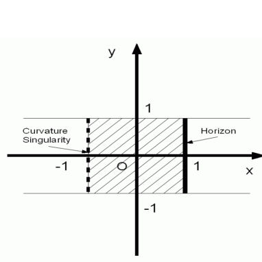
The point z = − z 0 𝑧 subscript 𝑧 0 z=-z_{0} z 𝑧 z ( ρ , z ) 𝜌 𝑧 (\rho,z) ( − z 0 / d , 1 ) subscript 𝑧 0 𝑑 1 (-z_{0}/d,1) ( z 0 / d , − 1 ) subscript 𝑧 0 𝑑 1 (z_{0}/d,-1) ( x , y ) 𝑥 𝑦 (x,y) [ − d , d ] 𝑑 𝑑 [-d,d] z 𝑧 z x = 1 𝑥 1 x=1 − 1 < y < 1 1 𝑦 1 -1<y<1 ( x , y ) 𝑥 𝑦 (x,y) − 1 < x < 1 1 𝑥 1 -1<x<1 − 1 < y < 1 1 𝑦 1 -1<y<1 ( ρ , z ) 𝜌 𝑧 (\rho,z) x = − 1 𝑥 1 x=-1
R α β γ δ R α β γ δ ∼ constant × z 0 − d y ( x + 1 ) 6 . similar-to superscript 𝑅 𝛼 𝛽 𝛾 𝛿 subscript 𝑅 𝛼 𝛽 𝛾 𝛿 constant subscript 𝑧 0 𝑑 𝑦 superscript 𝑥 1 6 \displaystyle R^{\alpha\beta\gamma\delta}R_{\alpha\beta\gamma\delta}\sim{\rm constant}\times\frac{z_{0}-dy}{(x+1)^{6}}. (205)
This curvature singularity is covered with the horizon of the dilaton black ring.
Figure 1: The horizon and the curvature singularity are depicted in the x 𝑥 x y 𝑦 y − 1 < x < 1 1 𝑥 1 -1<x<1 − 1 < y < 1 1 𝑦 1 -1<y<1 x = 1 𝑥 1 x=1
We next study the asymptotic behaviors of the metric components, the dilaton fields and the electric potential. Using
h ℎ \displaystyle h ∼ similar-to \displaystyle\sim 1 − 2 d ρ 2 + z 2 , 1 2 𝑑 superscript 𝜌 2 superscript 𝑧 2 \displaystyle 1-\frac{2d}{\sqrt{\rho^{2}+z^{2}}}, (206)
K 𝐾 \displaystyle K ∼ similar-to \displaystyle\sim 1 + 4 α 2 + 2 m − d ρ 2 + z 2 , 1 4 superscript 𝛼 2 2 𝑚 𝑑 superscript 𝜌 2 superscript 𝑧 2 \displaystyle 1+\frac{4}{\alpha^{2}+2}\frac{m-d}{\sqrt{\rho^{2}+z^{2}}}, (207)
as ρ 2 + z 2 → ∞ → superscript 𝜌 2 superscript 𝑧 2 \sqrt{\rho^{2}+z^{2}}\to\infty
g 00 ∼ − 1 , g 11 ∼ − z + ρ 2 + z 2 , formulae-sequence similar-to subscript 𝑔 00 1 similar-to subscript 𝑔 11 𝑧 superscript 𝜌 2 superscript 𝑧 2 \displaystyle g_{00}\sim-1,\quad g_{11}\sim-z+\sqrt{\rho^{2}+z^{2}}, (208)
g 22 ∼ z + ρ 2 + z 2 , f ∼ 1 2 ρ 2 + z 2 , formulae-sequence similar-to subscript 𝑔 22 𝑧 superscript 𝜌 2 superscript 𝑧 2 similar-to 𝑓 1 2 superscript 𝜌 2 superscript 𝑧 2 \displaystyle g_{22}\sim z+\sqrt{\rho^{2}+z^{2}},\quad f\sim\frac{1}{2\sqrt{\rho^{2}+z^{2}}}, (209)
which shows the metric becomes asymptotically flat, and the fields approach to
Φ Φ \displaystyle\Phi ∼ similar-to \displaystyle\sim − 3 α 2 ( α 2 + 2 ) m − d ρ 2 + z 2 , 3 𝛼 2 superscript 𝛼 2 2 𝑚 𝑑 superscript 𝜌 2 superscript 𝑧 2 \displaystyle-\frac{3\alpha}{2(\alpha^{2}+2)}\frac{m-d}{\sqrt{\rho^{2}+z^{2}}}, (210)
χ 𝜒 \displaystyle\chi ∼ similar-to \displaystyle\sim e ρ 2 + z 2 . 𝑒 superscript 𝜌 2 superscript 𝑧 2 \displaystyle\frac{e}{\sqrt{\rho^{2}+z^{2}}}. (211)
From Eq. (171 [ d , − z 0 ] 𝑑 subscript 𝑧 0 [d,-z_{0}] d = − z 0 𝑑 subscript 𝑧 0 d=-z_{0} △ x 2 = 2 π △ superscript 𝑥 2 2 𝜋 \triangle x^{2}=2\pi d = 0 𝑑 0 d=0 d = − z 0 𝑑 subscript 𝑧 0 d=-z_{0} g 00 , g 11 subscript 𝑔 00 subscript 𝑔 11
g_{00},g_{11} g 22 subscript 𝑔 22 g_{22} 189 191
h = − μ 1 μ ρ 2 , ℎ subscript 𝜇 1 𝜇 superscript 𝜌 2 \displaystyle h=-\frac{\mu_{1}\mu}{\rho^{2}}, (212)
and the component f 𝑓 f
f = K ρ 2 ( μ 1 − μ ) ( μ 1 2 + ρ 2 ) ( μ + ρ 2 ) , 𝑓 𝐾 superscript 𝜌 2 subscript 𝜇 1 𝜇 superscript subscript 𝜇 1 2 superscript 𝜌 2 𝜇 superscript 𝜌 2 \displaystyle f=\frac{\sqrt{K}\rho^{2}(\mu_{1}-\mu)}{(\mu_{1}^{2}+\rho^{2})(\mu+\rho^{2})}, (213)
where we have used the limit
lim d → − z 0 z 0 + d μ 2 − μ = − ( z + z 0 ) 2 + ρ 2 μ . subscript → 𝑑 subscript 𝑧 0 subscript 𝑧 0 𝑑 subscript 𝜇 2 𝜇 superscript 𝑧 subscript 𝑧 0 2 superscript 𝜌 2 𝜇 \displaystyle\lim_{d\to-z_{0}}\frac{z_{0}+d}{\mu_{2}-\mu}=-\frac{\sqrt{(z+z_{0})^{2}+\rho^{2}}}{\mu}. (214)
Introducing the hyper-spherical coordinates r 𝑟 r θ 𝜃 \theta
ρ 𝜌 \displaystyle\rho = \displaystyle= 1 2 ( r 2 − 2 m ) 2 − 4 d 2 sin 2 θ , 1 2 superscript superscript 𝑟 2 2 𝑚 2 4 superscript 𝑑 2 2 𝜃 \displaystyle\frac{1}{2}\sqrt{(r^{2}-2m)^{2}-4d^{2}}\sin 2\theta, (215)
z 𝑧 \displaystyle z = \displaystyle= 1 2 ( r 2 − 2 m ) cos 2 θ , 1 2 superscript 𝑟 2 2 𝑚 2 𝜃 \displaystyle\frac{1}{2}(r^{2}-2m)\cos 2\theta, (216)
we have
μ 𝜇 \displaystyle\mu = \displaystyle= − ( r 2 − 2 m − 2 d ) cos 2 θ , superscript 𝑟 2 2 𝑚 2 𝑑 superscript 2 𝜃 \displaystyle-(r^{2}-2m-2d)\cos^{2}\theta, (217)
μ ∗ superscript 𝜇 \displaystyle\mu^{*} = \displaystyle= ( r 2 − 2 m + 2 d ) sin 2 θ , superscript 𝑟 2 2 𝑚 2 𝑑 superscript 2 𝜃 \displaystyle(r^{2}-2m+2d)\sin^{2}\theta, (218)
μ 1 subscript 𝜇 1 \displaystyle\mu_{1} = \displaystyle= ( r 2 − 2 m − 2 d ) sin 2 θ , superscript 𝑟 2 2 𝑚 2 𝑑 superscript 2 𝜃 \displaystyle(r^{2}-2m-2d)\sin^{2}\theta, (219)
h ℎ \displaystyle h = \displaystyle= r 2 − 2 m − 2 d r 2 − 2 m + 2 d , superscript 𝑟 2 2 𝑚 2 𝑑 superscript 𝑟 2 2 𝑚 2 𝑑 \displaystyle\frac{r^{2}-2m-2d}{r^{2}-2m+2d}, (220)
K 𝐾 \displaystyle K = \displaystyle= ( r 2 r 2 − 2 m + 2 d ) 4 / ( α 2 + 2 ) . superscript superscript 𝑟 2 superscript 𝑟 2 2 𝑚 2 𝑑 4 superscript 𝛼 2 2 \displaystyle\left(\frac{r^{2}}{r^{2}-2m+2d}\right)^{4/(\alpha^{2}+2)}. (221)
By using these expressions the metric components are reduced to
g 00 subscript 𝑔 00 \displaystyle g_{00} = \displaystyle= − r 2 − 2 m − 2 d r 2 − 2 m + 2 d ( r 2 − 2 m + 2 d r 2 ) 4 / ( α 2 + 2 ) , superscript 𝑟 2 2 𝑚 2 𝑑 superscript 𝑟 2 2 𝑚 2 𝑑 superscript superscript 𝑟 2 2 𝑚 2 𝑑 superscript 𝑟 2 4 superscript 𝛼 2 2 \displaystyle-\frac{r^{2}-2m-2d}{r^{2}-2m+2d}\left(\frac{r^{2}-2m+2d}{r^{2}}\right)^{4/(\alpha^{2}+2)}, (222)
g 11 subscript 𝑔 11 \displaystyle g_{11} = \displaystyle= ( r 2 − 2 m + 2 d ) sin 2 θ ( r 2 r 2 − 2 m + 2 d ) 2 / ( α 2 + 2 ) , superscript 𝑟 2 2 𝑚 2 𝑑 superscript 2 𝜃 superscript superscript 𝑟 2 superscript 𝑟 2 2 𝑚 2 𝑑 2 superscript 𝛼 2 2 \displaystyle(r^{2}-2m+2d)\sin^{2}\theta\left(\frac{r^{2}}{r^{2}-2m+2d}\right)^{2/(\alpha^{2}+2)}, (223)
g 22 subscript 𝑔 22 \displaystyle g_{22} = \displaystyle= ( r 2 − 2 m + 2 d ) cos 2 θ ( r 2 r 2 − 2 m + 2 d ) 2 / ( α 2 + 2 ) , superscript 𝑟 2 2 𝑚 2 𝑑 superscript 2 𝜃 superscript superscript 𝑟 2 superscript 𝑟 2 2 𝑚 2 𝑑 2 superscript 𝛼 2 2 \displaystyle(r^{2}-2m+2d)\cos^{2}\theta\left(\frac{r^{2}}{r^{2}-2m+2d}\right)^{2/(\alpha^{2}+2)}, (224)
f 𝑓 \displaystyle f = \displaystyle= r 2 − 2 m + 2 d ( r 2 − 2 m ) 2 − 4 d 2 cos 2 2 θ ( r 2 r 2 − 2 m + 2 d ) 2 / ( α 2 + 2 ) . superscript 𝑟 2 2 𝑚 2 𝑑 superscript superscript 𝑟 2 2 𝑚 2 4 superscript 𝑑 2 superscript 2 2 𝜃 superscript superscript 𝑟 2 superscript 𝑟 2 2 𝑚 2 𝑑 2 superscript 𝛼 2 2 \displaystyle\frac{r^{2}-2m+2d}{(r^{2}-2m)^{2}-4d^{2}\cos^{2}2\theta}\left(\frac{r^{2}}{r^{2}-2m+2d}\right)^{2/(\alpha^{2}+2)}. (225)
Then, noting the relation
d ρ 2 + d z 2 = [ ( r 2 − 2 m ) 2 − 4 d 2 cos 2 2 θ ] [ r 2 d r 2 ( r 2 − 2 m ) 2 − 4 d 2 + d θ 2 ] , 𝑑 superscript 𝜌 2 𝑑 superscript 𝑧 2 delimited-[] superscript superscript 𝑟 2 2 𝑚 2 4 superscript 𝑑 2 superscript 2 2 𝜃 delimited-[] superscript 𝑟 2 𝑑 superscript 𝑟 2 superscript superscript 𝑟 2 2 𝑚 2 4 superscript 𝑑 2 𝑑 superscript 𝜃 2 \displaystyle d\rho^{2}+dz^{2}=\left[(r^{2}-2m)^{2}-4d^{2}\cos^{2}2\theta\right]\left[\frac{r^{2}dr^{2}}{(r^{2}-2m)^{2}-4d^{2}}+d\theta^{2}\right], (226)
we obtain
d s 2 = 𝑑 superscript 𝑠 2 absent \displaystyle ds^{2}= − \displaystyle- [ 1 − 2 ( m + d ) r 2 ] Y − ( α 2 − 2 ) / ( α 2 + 2 ) ( d x 0 ) 2 delimited-[] 1 2 𝑚 𝑑 superscript 𝑟 2 superscript 𝑌 superscript 𝛼 2 2 superscript 𝛼 2 2 superscript 𝑑 superscript 𝑥 0 2 \displaystyle\left[1-\frac{2(m+d)}{r^{2}}\right]Y^{-(\alpha^{2}-2)/(\alpha^{2}+2)}(dx^{0})^{2} (227)
+ \displaystyle+ [ 1 − 2 ( m + d ) r 2 ] − 1 Y − 2 / ( α 2 + 2 ) d r 2 superscript delimited-[] 1 2 𝑚 𝑑 superscript 𝑟 2 1 superscript 𝑌 2 superscript 𝛼 2 2 𝑑 superscript 𝑟 2 \displaystyle\left[1-\frac{2(m+d)}{r^{2}}\right]^{-1}Y^{-2/(\alpha^{2}+2)}dr^{2} (228)
+ \displaystyle+ Y α 2 / ( α 2 + 2 ) r 2 [ d θ 2 + sin 2 θ ( d x 1 ) 2 + cos 2 θ ( d x 2 ) 2 ] , superscript 𝑌 superscript 𝛼 2 superscript 𝛼 2 2 superscript 𝑟 2 delimited-[] 𝑑 superscript 𝜃 2 superscript 2 𝜃 superscript 𝑑 superscript 𝑥 1 2 superscript 2 𝜃 superscript 𝑑 superscript 𝑥 2 2 \displaystyle Y^{\alpha^{2}/(\alpha^{2}+2)}r^{2}[d\theta^{2}+\sin^{2}\theta(dx^{1})^{2}+\cos^{2}\theta(dx^{2})^{2}], (229)
where
Y = 1 − 2 ( m − d ) r 2 . 𝑌 1 2 𝑚 𝑑 superscript 𝑟 2 \displaystyle Y=1-\frac{2(m-d)}{r^{2}}. (230)
This metric has an event horizon at r 2 = 2 ( m + d ) superscript 𝑟 2 2 𝑚 𝑑 r^{2}=2(m+d) r 2 = 2 ( m − d ) superscript 𝑟 2 2 𝑚 𝑑 r^{2}=2(m-d) [23 ] . The difference from their solution comes from the imposition of the coordinate condition det g = − ρ 2 𝑔 superscript 𝜌 2 \det g=-\rho^{2}
g 00 ⋅ g r r = − Y − α 2 / ( α 2 + 2 ) , ⋅ subscript 𝑔 00 subscript 𝑔 𝑟 𝑟 superscript 𝑌 superscript 𝛼 2 superscript 𝛼 2 2 \displaystyle g_{00}\cdot g_{rr}=-Y^{-\alpha^{2}/(\alpha^{2}+2)}, (231)
which does not equal to − 1 1 -1 d = 0 𝑑 0 d=0 r 2 = 2 m superscript 𝑟 2 2 𝑚 r^{2}=2m
The second possibility of removing the conical singularity is setting d = 0 𝑑 0 d=0 d = 0 𝑑 0 d=0 z 0 ≠ 0 subscript 𝑧 0 0 z_{0}\neq 0
g 00 subscript 𝑔 00 \displaystyle g_{00} = \displaystyle= − K 0 − 1 , superscript subscript 𝐾 0 1 \displaystyle-K_{0}^{-1}, (232)
g 11 subscript 𝑔 11 \displaystyle g_{11} = \displaystyle= μ ∗ K 0 , superscript 𝜇 subscript 𝐾 0 \displaystyle\mu^{*}\sqrt{K_{0}}, (233)
g 22 subscript 𝑔 22 \displaystyle g_{22} = \displaystyle= − μ K 0 , 𝜇 subscript 𝐾 0 \displaystyle-\mu\sqrt{K_{0}}, (234)
f 𝑓 \displaystyle f = \displaystyle= K 0 2 ( z + z 0 ) 2 + ρ 2 , subscript 𝐾 0 2 superscript 𝑧 subscript 𝑧 0 2 superscript 𝜌 2 \displaystyle\frac{\sqrt{K_{0}}}{2\sqrt{(z+z_{0})^{2}+\rho^{2}}}, (235)
where
K 0 = ( 1 + m ρ 2 + z 2 ) 4 / ( α 2 + 2 ) . subscript 𝐾 0 superscript 1 𝑚 superscript 𝜌 2 superscript 𝑧 2 4 superscript 𝛼 2 2 \displaystyle K_{0}=\left(1+\frac{m}{\sqrt{\rho^{2}+z^{2}}}\right)^{4/(\alpha^{2}+2)}. (236)
We find that the solution has a ring-like structure at z = 0 𝑧 0 z=0
g 00 subscript 𝑔 00 \displaystyle g_{00} ∼ similar-to \displaystyle\sim ρ 4 / ( α 2 + 2 ) , superscript 𝜌 4 superscript 𝛼 2 2 \displaystyle\rho^{4/(\alpha^{2}+2)}, (237)
g 22 subscript 𝑔 22 \displaystyle g_{22} ∼ similar-to \displaystyle\sim ρ 2 ( α 2 + 1 ) / ( α 2 + 2 ) . superscript 𝜌 2 superscript 𝛼 2 1 superscript 𝛼 2 2 \displaystyle\rho^{2(\alpha^{2}+1)/(\alpha^{2}+2)}. (238)
This shows that there are two eigenvectors belonging to the zero eigenvalue for g 𝑔 g ρ = 0 𝜌 0 \rho=0 z = 0 𝑧 0 z=0