Direct Detection of the Close Companion of Polaris with the Hubble Space Telescope

Abstract

Polaris, the nearest and brightest classical Cepheid, is a single-lined spectroscopic binary with an orbital period of 30 years. Using the High Resolution Channel of the Advanced Camera for Surveys onboard the Hubble Space Telescope (HST) at a wavelength of $\sim$2255 Å, we have directly detected the faint companion at a separation of $0\farcs 17$. A second HST observation 1.04 yr later confirms orbital motion in a retrograde direction. By combining our two measures with the spectroscopic orbit of Kamper and an analysis of the Hipparcos and FK5 proper motions by Wielen et al., we find a mass for Polaris Aa of $4.5^{+2.2}_{-1.4}\,M_{\odot}$—the first purely dynamical mass determined for any Cepheid. For the faint companion Polaris Ab we find a dynamical mass of $1.26^{+0.14}_{-0.07}\,M_{\odot}$, consistent with an inferred spectral type of F6 V and with the flux difference of 5.4 mag observed at 2255 Å. The magnitude difference at the $V$ band is estimated to be 7.2 mag. Continued HST observations will significantly reduce the mass errors, which are presently still too large to provide critical constraints on the roles of convective overshoot, mass loss, rotation, and opacities in the evolution of intermediate-mass stars.

Our astrometry, combined with two centuries of archival measurements, also confirms that the well-known, more distant ($18^{\prime\prime}$) visual companion, Polaris B, has a nearly common proper motion with that of the Aa,Ab pair. This is consistent with orbital motion in a long-period bound system. The ultraviolet brightness of Polaris B is in accordance with its known F3 V spectral type if it has the same distance as Polaris Aa,Ab.

1 Introduction

Cepheid variable stars are of central importance in galactic and extragalactic astronomy. They are the primary standard candles for measuring extragalactic distances, and they provide critical tests of stellar-evolution theory. Surprisingly, however, until now there has not been a single Cepheid with a purely dynamical measurement of its mass.

Polaris ($\alpha$ UMi) is the nearest and, at 2nd magnitude, the brightest classical Cepheid, albeit one with a small light amplitude in its 3.97-day pulsation period (Turner et al. 2005 and references therein). The amplitude, which had been decreasing for several decades, now appears to have stabilized and may be increasing again (Bruntt et al. 2008 and references therein). The Hipparcos parallax of Polaris indicates a luminosity consistent with pulsation in the first overtone (Feast & Catchpole 1997).

Polaris is the brightest member of a triple system (see Kamper 1996 and references therein). The well-known visual companion, Polaris B, is an 8th-magnitude F3 V star at a separation of $18^{\prime\prime}$. The Cepheid itself is a member of a single-lined spectroscopic binary with a period of 30 yr. In this paper we report the first direct detection of the close companion, from which we derive the first entirely dynamical mass measurement for a Cepheid.

Cepheid masses are a key parameter for testing stellar evolutionary calculations. Beginning in the 1960’s, discrepancies were found in the sense that Cepheid masses derived from pulsation modeling were lower than those derived from evolutionary tracks. A revision in envelope opacities brought pulsation and evolutionary masses closer together, partially alleviating this “Cepheid mass problem.” However, recent evolutionary and pulsation constraints for Galactic (Bono et al. 2001b; Caputo et al. 2005; Keller 2008; Natale, Marconi, & Bono 2008) and Magellanic (Bono, Castellani, & Marconi 2002; Keller & Wood 2006) Cepheids still imply a discrepancy in masses at the $\sim$15-20% level. The luminosities of Cepheids depend on the mass of the helium-burning core; physical mechanisms affecting the helium core mass include mixing due to convective core overshoot during the main-sequence phase, mass loss, stellar rotation, and radiative opacity. A directly measured mass for Polaris would thus provide an important constraint on this theoretical framework.

2 Observations and Data Reduction

With the intention of a direct detection of the close companion, we imaged Polaris with the Hubble Space Telescope (HST) and the High Resolution Channel (HRC; plate scale $0\farcs 026\,\rm pixel^{-1}$) of the Advanced Camera for Surveys (ACS). We chose the ultraviolet F220W filter (effective wavelength $\sim$2255 Å) in order to minimize the contrast between Polaris and the close companion, which we anticipated to be a main-sequence star slightly hotter than the Cepheid, and also to minimize the size of the point-spread function (PSF).

Observations were obtained on 2005 August 2-3, and again on 2006 August 13. At the first epoch we obtained a series of 0.1 to 0.3 s exposures dithered across 200 pixels on the chip over the course of one HST orbit, with several exposures taken at each dither position. At the second epoch we used the same dither pattern, but divided the spacecraft orbit between a series of 0.3 s exposures on Polaris A and 20 s exposures on Polaris B. For the longer exposures, we placed Polaris B at the same chip location as Polaris A in the short exposures, so as to provide an accurate PSF for a single star at the same place in the field of view.

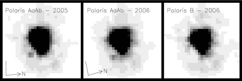
Figure 1: Coadded ACS HRC images of Polaris Aa,Ab taken with the F220W filter on 2005 Aug 2 (left) and 2006 Aug 13 (middle). The close companion Ab is detected at the lower left of the primary (at about a “7 o’clock” position). The images are $0\farcs 85\times 0\farcs 85$ and the directions of N and E are indicated. The right-hand panel shows a coadded image of Polaris B from longer exposures taken during the 2006 observations, and scaled to the flux level of the Polaris Aa,Ab images. There is no artifact in the Polaris B PSF at the location of Ab.

Figure 1 shows the co-added images of Polaris A from 2005 (left panel) and 2006 (middle panel). The close companion (which we designate Polaris Ab) is detected at the lower left of the primary (at about a “7 o’clock” position). Because of the asymmetric PSF shape, we performed several checks to confirm that the apparent companion is not an artifact. The right-hand frame in Figure 1 shows Polaris B in the 2006 image, with the star shifted to the same field position as Polaris A, and with its image scaled to the same flux as Polaris A. This PSF shows no artifact at the location of the companion seen in the images of Polaris A.

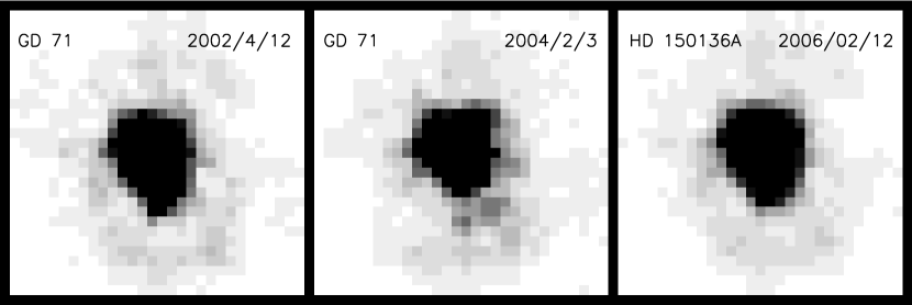
Figure 3: Archival images of flux-calibration standard stars observed with the ACS/HRC in the F220W filter. The star names and dates of observation are listed in each panel. There is no artifact at the location of the Polaris Ab companion.

Figure 2 shows contour maps of the same three images. Again the faint companion is seen in the 2005 and 2006 images of Polaris A, and there is no PSF artifact at this location in the image of Polaris B. We also retrieved images from the HST archive of several standard stars observed with ACS/HRC in the F220W filter over an interval of four years. Examples of these observations are shown in Figure 3. Although the PSF structure does vary somewhat with time, due to small changes in telescope focus and other instrumental phenomena, none of these images show any artifact at the location of the Polaris Ab companion seen in Figures 1 and 2.

To measure the separation and position angle between Polaris Aa and the newly revealed close companion, we used the calibrated flat-fielded exposures provided by the HST reduction pipeline. At each dither location, we median-filtered the repeated observations to remove cosmic rays. We then extracted subarrays from the images centered on Polaris Aa with a size of $0\farcs 85\times 0\farcs 85$. We used the observations of Polaris B from 2006 as a reference PSF to construct models of the close pair (Aa,Ab) by searching through a grid of separations and flux ratios. The IDL interpolate procedure was used to shift the PSF by sub-pixel intervals, using cubic convolution interpolation. The background was least-squares fitted with a tilted plane.

The separations, position angles (PAs), and magnitude differences, determined through $\chi^{2}$ minimization between the models and the observations, are given in Table 1. The uncertainties were determined by analyzing multiple images individually and computing the standard deviation. We applied the filter-dependent geometric distortion correction of Anderson & King (2004) to convert the pixel values to a separation in arcseconds. To define the orientation of the detector $y$-axis on the sky, and thus determine the PA of the binary relative to the pole for the equinox J2000.0, we used the HST image-header keyword PA_APER.

We also measured the separation and PA of the wide companion, Polaris B, relative to Aa, and the results are presented in Table 2. The good agreement with the historical measurements of the PA of Polaris B relative to A (see §4) indicates that we are properly defining the direction of north in spite of the extreme northerly declination. (Since the historical double-star convention is to give the PA for the equinox of the date of observation, we computed the precession corrections and give the adjusted PAs in the footnotes to Tables 1 and 2, for the convenience of archivists.)

3 Orbital Solutions

We stress that the orbital analyses discussed below are only preliminary fits to data with a very limited sample (only two points) of separations and PAs. We followed three different approaches to determining the orbital parameters, in order to illustrate the scope of the available data.

Kamper (1996) rederived the single-lined spectroscopic orbit of Polaris Aa using improved radial-velocity data, and a careful removal of the velocity signal due to the Cepheid pulsation. His solution provides the period, time of periastron passage, eccentricity, angle between the node and periastron, and the radial-velocity semi-amplitude of the primary (denoted $P,T,e,\omega,$ and $K_{\rm Aa}$, respectively). By comparing the Hipparcos proper motion of Polaris Aa (which, over the duration of the Hipparcos mission, is nearly instantaneous in the context of the 30-year orbit) with the ground-based long-term average proper motion from the FK5 (which is essentially the motion of the center of mass), Wielen et al. (2000) determined the inclination and the PA of the line of nodes ($i$ and $\Omega$). Their analysis, however, allows for retrograde and prograde orbital solutions (the two orbits being tangential at the Hipparcos epoch), with two different values of $i$ and $\Omega$. The orbital parameters based on the Kamper (1996) and the two Wielen et al. (2000) solutions are presented in Table 3.

The HST detection of the close companion Ab and its orbital motion at two epochs establishes a retrograde sense for the orbit (thus confirming the strong preference stated by Wielen et al. for their retrograde solution). Additionally, it provides constraints on the remaining unknown parameter of the orbit, the semi-major axis $a$. A combination of the spectroscopic mass function,

$$f(M)=(M_{\rm Ab}\sin{i})^{3}/(M_{\rm Aa}+M_{\rm Ab})^{2}=3.784\times 10^{-5}K_{\rm Aa}^{3}P(1-e^{2})^{3/2}\,,$$

with the total mass from Kepler’s Third Law,

$$M_{\rm tot}=M_{\rm Aa}+M_{\rm Ab}=\frac{a^{3}}{\pi^{3}P^{2}}\,,$$ (1)

then yields the masses of the binary components,

$$M_{\rm Ab}=0.03357\frac{K_{\rm Aa}a^{2}\sqrt{1-e^{2}}}{\pi^{2}P\sin{i}}\,,$$

$$M_{\rm Aa}=M_{\rm tot}-M_{\rm Ab}\,,$$

where $a$ and the parallax $\pi$ are in arcseconds, $P$ is in years, $K_{\rm Aa}$ is in km s^-1, and the masses are in $M_{\odot}$.

In §3.1-3.3 we describe the orbital fits that we computed based on a synthesis of the spectroscopic, astrometric, and HST data. In these sections, we present three successively more comprehensive orbital solutions. Table 4 summarizes the orbital parameters determined from each of these fits; the individual columns are described in more detail in §3.1-3.3.

3.1 Semi-major Axis

As a first approximation to an orbital solution, we fixed the spectroscopic and astrometric parameters ($P,T,e,\omega,i,\Omega$) to be those determined by Kamper (1996) and Wielen et al. (2000), and solved only for the semi-major axis $a$ based on the two HST separation measurements. The orbital parameters for this solution are listed in the second column of Table 4. Figure 4 compares this retrograde orbit fit with the HST measurements, and shows extremely poor agreement for the PAs. However, the relatively large uncertainties in $i$ and $\Omega$ determined by Wielen et al. (2000) provide considerable flexibility for adjusting the orbital parameters in order to improve the fit quality.

3.2 Best Fit to the HST Measurements

To get a better fit to the HST data, we solved for $i$, $\Omega$, and $a$ based on the two separation and PA measurements from the HST observations, while holding the relatively well-determined spectroscopic parameters ($P,T,e,$ and $\omega$) fixed. We computed the orbit fit through a standard Newton-Raphson method in $\chi^{2}$ space, and present the results in the third column of Table 4.

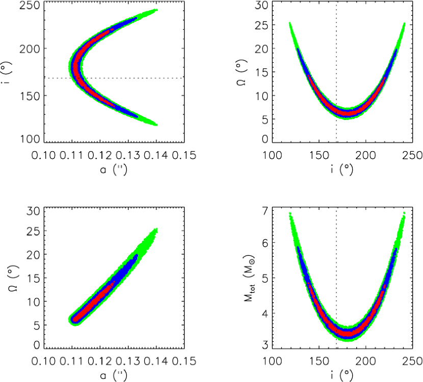
Figure 5: Crosscuts through the $\chi^{2}$ surfaces derived from the fit to the HST measurements alone while holding the spectroscopic parameters fixed. These results were obtained by performing a Monte-Carlo search for orbital solutions within the $3\sigma$ confidence interval ($\Delta\chi^{2}=9$). The total mass was derived for each of the 10,000 orbits found within this interval using a parallax of 7.72 mas. The dotted lines indicate the critical value of the inclination ($i=168^{\circ}$), above which negative values of a component mass are produced. The color codes in the electronic version of this figure correspond to the $1\sigma$ (red), $2\sigma$ (blue), and $3\sigma$ (green) confidence intervals.

To explore the range of orbital parameters that fit the HST data, we performed a Monte Carlo search by selecting values of $i$, $\Omega$, and $a$ at random. We searched for 10,000 solutions within the 3$\sigma$ confidence interval, corresponding to a difference of $\Delta\chi^{2}=9$ from the minimum $\chi^{2}$ value. Figure 5 shows cross-cuts through the $\chi^{2}$ surfaces for the three derived parameters. Using the recently revised Hipparcos parallax of $7.72\pm 0.12$ mas (van Leeuwen et al. 2007), we computed the total mass of the binary through Kepler’s Third Law for all of the solutions found in the Monte Carlo search. In the last panel of Figure 5 we show a plot of the total mass versus inclination. Because a visual orbit is insensitive to the individual masses of the components, when combining the total mass with the spectroscopic mass function, there exist values of the inclination that produce negative masses for $M_{\rm Aa}$ or $M_{\rm Ab}$. In the remaining analysis we removed these negative-mass solutions from our sample of possible orbits. Essentially, this rejects all orbital solutions with $i>168^{\circ}$. The 1$\sigma$ uncertainties listed in the third column of Table 4 are determined from the $\Delta\chi^{2}=1$ confidence interval of the modified distribution. The values of $i$ and $\Omega$ agree with the retrograde parameters computed by Wielen et al. (2000) at the 1.5$\sigma$ and 2.2$\sigma$ levels respectively. Figure 6 shows three examples illustrating how the orbit fit varies within a 1$\sigma$ confidence interval.

We note that the HST-only solution yields a secondary mass of $M_{\rm Ab}=1.8\,M_{\odot}$ (Table 4, col. 3), corresponding approximately to an A5 V star. The discussion below in §5.1, as well as the lack of a detection of the companion in UV spectra obtained by Evans (1988) with the International Ultraviolet Explorer (IUE), makes it highly improbable that Ab could be this hot. With only two HST measurements sampling the orbit thus far, we do not yet have a good constraint on the curvature, and hence acceleration, of the orbit. In turn, this limits how well we can determine the total system mass, and it contributes to the large errors quoted in Table 4.

3.3 Joint Fit to HST and Proper-Motion Measurements

Incorporation of the Hipparcos proper-motion measurements into the orbital fit extends the time coverage of the measurements to $\sim$15 years. This represents a significant fraction of the orbital period and is therefore likely to improve the reliability of the results. Following the technique described in Wielen et al. (2000), we performed a simultaneous fit to the proper-motion data and the HST measurements.

As Wielen et al. point out, the FK5 proper motion is averaged over several cycles of the orbital period and therefore reflects the center-of-mass motion of Polaris Aa,Ab. Because of the shorter time span of the Hipparcos mission, the Hipparcos proper motion more nearly represents an instantaneous measurement of the combined proper motion of the center of mass of the Aa,Ab pair and the orbital motion of the photocenter about the center of mass at the epoch of the observations ($\sim$1991.3). The difference between the FK5 and Hipparcos proper motions thus gives the offset caused by the orbital motion.

In computing the joint fit, we held the spectroscopic parameters ($P,T,e,\omega$, and $K_{\rm Aa}$) fixed at the Kamper (1996) values and solved for $i$, $\Omega$, and $a$, again using a Newton-Raphson technique in $\chi^{2}$ space. The input data were the relative positions of Aa and Ab at the two HST epochs, and the difference between the Hipparcos and FK5 proper motions. To incorporate the proper-motion data into the orbit fit, we had to compute the time-dependent offset of the photocenter relative to the center of mass predicted by the orbital parameters during the time of the Hipparcos observations. To compute these offsets, we converted the semi-major axis of Polaris Aa determined from the single-lined spectroscopic orbit to the semi-major axis of the photocenter by using the mass ratio computed from the full set of orbital parameters and a magnitude difference between Aa and Ab of $\Delta V=7.2$ (see §5.1). This conversion is specified by eqns. (8) and (9) in Wielen et al. (2000). The expected difference between the instantaneous and the mean proper motion ($\Delta\mu_{\rm fit}$) at the central epoch of the Hipparcos observations is then computed from eqn. (18) of Wielen et al.

Table 5 shows the values of the proper motions used by Wielen et al. (2000). The first line shows the proper motion of Polaris given in the FK5 catalog ($\mu_{\rm FK5}$). In the second line, a systematic correction is applied to convert the proper motion from the FK5 reference system to the Hipparcos/ICRS system (Wielen et al. 2000). The proper motion measured by Hipparcos ($\mu_{HIP}$) is given in the third line. The difference in the measured proper motions $\Delta\mu=\mu_{HIP}-\mu_{\rm FK5}$ is given in the fourth line.

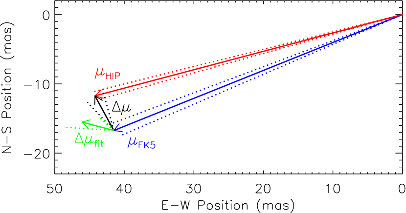
Figure 7: Schematic comparison between the instantaneous and mean proper motions of Polaris A. The vectors indicate the magnitude and direction of the annual proper-motion measurements from Hipparcos ($\mu_{\rm HIP}$; red), the long-term average FK5 ground-based motion ($\mu_{\rm FK5}$; blue), and the vector difference between the two ($\Delta\mu$; black). Dotted red and blue lines indicate the $1\sigma$ uncertainties in the Hipparcos and FK5 measurements. The green vector represents the best-fit difference between the proper motions ($\Delta\mu_{\rm fit}$) computed from our simultaneous orbit fit to the HST measurements and the proper-motion data while holding the spectroscopic parameters fixed (see §3.3).

The last line in Table 5 shows the best-fit difference between the instantaneous and mean proper motion ($\Delta\mu_{\rm fit}$) calculated from our simultaneous fit to the relative separation and PA measurements of Polaris Aa,Ab and the proper-motion data. Figure 7 shows a graphical representation of the Hipparcos and FK5 proper motions, and compares our best-fit value with the measured value for the difference between the instantaneous and mean proper motions.

As Figure 7 illustrates, the best-fit value of $\Delta\mu$ in right ascension agrees well ($0.7\sigma$) with the measured value, but the agreement is poorer ($3.2\sigma$) in declination. This discrepancy probably arises from our constraining the spectroscopic parameters to be exactly those derived by Kamper (1996), thus forcing the proper motions and HST measurements to absorb the errors. We found that by allowing some variation in the spectroscopic parameters, we could substantially improve the fit to the proper-motion measurements. Once we have sampled enough of the visual orbit to better constrain $i$, $\Omega$, and $a$, the optimal orbital solution should be found by doing a simultaneous fit to the radial-velocity, HST, and proper-motion data. Unfortunately, however, Kamper only tabulated the radial velocities before removal of the pulsational variation, so a re-computation of the pulsation corrections would have to be carried out—a task well beyond the scope of this paper, and one that should await the availability of more HST observations.

The orbital parameters and derived masses from our final combined fit are given in the last column of Table 4, which also contains our final best estimates for the dynamical masses of both stars. The best-fit orbit of Polaris Ab relative to Aa is plotted in Figure 8. The shaded-gray portion of the orbit marks the location of the companion during the interval of the Hipparcos observations in the early 1990’s, and it should be noted that the direction of motion at that time was, of course, $180^{\circ}$ different from the direction of the differential motion of Polaris Aa ($\Delta\mu_{\rm fit}$) shown as a green arrow in Figure 7.

4 Astrometry of Polaris B

Visual measurements of the PA and separation of the wide companion Polaris B relative to Polaris A extend back to the early 19th Century, with a few photographic observations being available from the 20th Century. We have compiled these measurements from Kamper (1996) and the Washington Double Star Catalog (Mason et al. 2001).

In Figure 9 we plot the PA measurements of Polaris B, which have been precessed to the J2000.0 equinox. Due to its slow relative motion and large magnitude difference, Polaris A,B was generally not included in the major double-star observing programs, especially in the latter half of the 20th Century. This had the consequence that most of the measures that were obtained tended to be made by less-experienced observers, often using older techniques and/or smaller telescopes; this may explain the surprisingly large scatter in the late 20th Century. A linear least-squares fit to the data yields a rate of change in the PA of $-0\fdg 00035\pm 0\fdg 00094{\rm~{}yr^{-1}}$, consistent with no detectable change in PA for the past two centuries. (The earlier work of Kamper had given a marginal detection of $+0\fdg 0086\pm 0\fdg 0076{\rm~{}yr^{-1}}$.)

The separation measurements for Polaris B are plotted in Figure 10. There has been a slow downward trend in the separation, with a least-squares fit giving a rate of $-1.67\pm 0.19$ mas yr^-1. Kamper (1996), from the ground-based measures only, had found $-1.7\pm 0.6$ mas yr^-1. Since the absolute proper motion of Polaris A is $\sim$46 mas yr^-1 (see Table 5), the absolute motions of A and B agree to within about 4%. At the distance of Polaris given by the Hipparcos parallax, the difference in tangential velocities between A and B is $1.03\pm 0.12\,\rm km\,s^{-1}$.

In computing these least-squares fits, we weighted the observations by estimates of their measurement errors. For the HST observations, we applied the uncertainties quoted in Table 2. For the historical measurements, we divided the data into four groups spanning approximately 50 years each. We assumed measurement uncertainties equal to the standard deviation of the values measured in each of these four groups.

The slowly diminishing separation of A and B (at constant PA) is not inconsistent with orbital motion in a physically bound pair—which is also supported by the close similarities of the radial velocities of A and B (Kamper 1996; Usenko & Klochkova 2007). To predict an order-of-magnitude rate of change in the separation, we assumed a circular orbit with a total system mass of $M_{\rm Aa}+M_{\rm Ab}+M_{\rm B}=7.15\,M_{\odot}$ (based on the Aa+Ab mass of $5.8\,M_{\odot}$ in the last column of Table 4 and a mass for Polaris B of $1.35\,M_{\odot}$—see below). Adopting the revised Hipparcos parallax of 7.72 mas, and assuming an edge-on orbit with a period of $\sim$100,000 yr, we find a semimajor axis of $a\simeq 32^{\prime\prime}$ (or 0.02 pc). At the orbital phase implied by the observed separation of $18\farcs 2$, the relative motion would then be $-1.65$ mas yr^-1, close to the observed value.

5 Astrophysical Properties of the Companions of Polaris

5.1 Polaris Ab

Our observed ultraviolet magnitude difference between Polaris Aa and Ab may be used to infer the spectral type, and hence the mass, of the newly resolved close companion.

We downloaded UV spectra from the IUE data archive for three F-type dwarfs having accurate spectral types and parallaxes, as well as for Polaris itself. The F stars selected were 78 UMa (HR 4931, HD 113139; F2 V), HD 27524 (F5 V), and HD 27808 (F8 V). The latter two stars (Hyades members), as well as Polaris itself, were taken to be unreddened, while the spectrum of 78 UMa (a member of the Ursa Major group) was dereddened by $E(B-V)=0.01$ mag. We then scaled the flux distributions for the three stars to the distance of Polaris, using the respective Hipparcos parallaxes.

In Table 6, we list these comparison stars, their spectral types, masses implied by the spectral types, their Hipparcos parallaxes, absolute magnitudes based on the parallaxes, and finally the predicted flux ratios relative to Polaris in the ACS/HRC F220W band. The adopted relationship between spectral types and masses is that of Harmanec (1988). The flux ratios were calculated by convolving the F220W system-throughput function (see Chiaberge & Sirianni 2007) with the scaled IUE spectra, and then ratioing with respect to Polaris. In Figure 11 we show the IUE spectrum of Polaris and the scaled spectra of the three F dwarfs.

As listed in Table 1, the observed magnitude difference in the ACS/HRC F220W filter between Polaris Aa and Ab is $5.39\pm 0.08$ mag, or a flux ratio of $0.0070\pm 0.0006$. A small correction to this ratio is needed because of the small ($\sim$10-15%) contribution to the signal from the red leak in the F220W filter, Polaris Aa being slightly redder than the companion. The red-leak contributions have been tabulated as a function of spectral type by Chiaberge & Sirianni (2007), leading to a corrected in-band flux ratio of $0.0074\pm 0.0006$. This value is entered in the fourth row of Table 6, and is marked with a horizontal line in Figure 11. Interpolation in the last column of Table 6 then leads to an inferred spectral type of about F6 V, an absolute visual magnitude of $M_{V}\simeq+3.6$, and an expected mass of $1.3\,M_{\odot}$.

The apparent $V$-band magnitude of Polaris Ab, for a distance modulus $(m-M)_{0}=5.56$, is inferred to be about 9.2, or some 7.2 mag fainter at $V$ than Polaris Aa. This illustrates the advantage of observing the Polaris system in the ultraviolet, which lessens the contrast by nearly 2 mag.

5.2 Polaris B

As listed in Table 2, we also measured the F220W flux difference between Polaris Aa and B as $4.49\pm 0.04$ mag, or a flux ratio of $0.0160\pm 0.0006$. Correction for red leak, as described above, changes the flux ratio to $0.0178\pm 0.0006$, entered in the second row of Table 6, and also marked with a horizontal line in Figure 11. Interpolating again in the table, we see that this ratio corresponds to a star intermediate between types F3 V and F4 V. In the case of the well-resolved Polaris B the optical spectral type has been determined from the ground. Our result is in gratifying agreement with the spectral type of F3 V found by Turner (1977) and Usenko & Klochkova (2007), who also cite earlier spectral classifications of Polaris B by experts such as Bidelman. This finding not only validates our photometric analysis of Polaris Ab above, but again supports the physical association of Polaris A and B. Based on the relationship between spectral type and mass in Table 6, we infer the mass of Polaris B to be near $1.35\,M_{\odot}$.

Using the same method as for Polaris Ab, we can use the UV flux ratio to infer the $V$ magnitude of Polaris B to be 8.7. The visual magnitude of Polaris B can be measured from the ground, but is made difficult by scattered light from Polaris A. Kamper (1996) used CCD imaging to determine a magnitude difference with respect to A of $\Delta V=6.61$, implying $V=8.59$ (in good agreement with earlier photoelectric measurements of $V=8.5$ and 8.60 by Fernie 1966 and McNamara 1969, respectively; Fernie included an approximate correction for scattered light, and McNamara states that he observed only on excellent nights). In more recent work, to be reported separately, we have been carrying out astrometry of Polaris B with the Fine Guidance Sensors (FGS) onboard HST. As a byproduct, these observations yield an accurate $V$ magnitude of $8.65\pm 0.02$. Thus our indirectly inferred $V$ magnitude for Polaris B of 8.7 agrees very well with the ground- and HST-based observations.

6 Dynamical Masses

6.1 Polaris Ab

The final column in Table 4 lists the dynamical masses of both components of the close pair Aa,Ab obtained from our final orbital solution, as described in §3.3. For Ab, the dynamical mass is $1.26^{+0.14}_{-0.07}\,M_{\odot}$. This is in remarkably good agreement with the $1.3\,M_{\odot}$ inferred indirectly from the UV flux difference (§5.1), and is an indicator of the validity of our orbital solution.

6.2 Theoretical Implications of the Cepheid’s Dynamical Mass

The dynamical mass of the Cepheid Polaris Aa from our final orbital solution, as listed in the last column in Table 4, is $4.5^{+2.2}_{-1.4}\,M_{\odot}$.

We compare this result first with theoretical “evolutionary” masses, $M_{e}$. The input data are the intensity-averaged mean apparent magnitudes ($m_{V}=1.98$, $m_{B}=2.58$, from Fernie et al. 1995 and assumed to be unreddened), the revised Hipparcos distance of $129.5\pm 2.0$ pc (van Leeuwen et al. 2007), and a solar metal abundance (Luck & Bond 1986; Usenko et al. 2005). We adopt the mass-period-luminosity (MPL) relation for He-burning fundamental pulsators provided by Caputo et al. (2005, their Table 4). Before using this relation, we fundamentalized the first-overtone (FO) pulsation period of Polaris with the relationship $\log P_{\rm F}=\log P_{\rm FO}+0.13$. By assuming Cepheid luminosities predicted by “canonical” evolutionary models that neglect convective-core overshooting, we find $M_{e}=6.1\pm 0.4\,M_{\odot}$. On the other hand, if we assume luminosities predicted by “noncanonical” evolutionary models that account for mild convective-core overshooting, given by $L/L_{\rm can}\simeq 1.3$, we find $M_{e}=5.6\pm 0.4\,M_{\odot}$. Use of the mass-color-luminosity (MCL) relation (Caputo et al. 2005, Table 5) yields very similar evolutionary masses.

The HR diagrams in Figure 12 show a direct comparison between theoretical evolutionary tracks and observations in the $M_{V},(B-V)_{0}$ plane. In both panels of Figure 12 we plot the location of Polaris with an open triangle enclosing a small error bar. The top panel shows canonical evolutionary tracks at solar chemical composition; $M_{e}\simeq 6\,M_{\odot}$ provides a good fit to the position of Polaris. The bottom panel shows noncanonical tracks, suggesting $M_{e}\simeq 5.5\,M_{\odot}$, except that the tip of the blue loop is not quite as hot as Polaris. However, the blueward extension of the loops is affected by chemical composition and by physical and numerical assumptions (Stothers & Chin 1991; Chiosi, Bertelli, & Bressan 1992; Bono et al. 2000; Meynet & Maeder 2000; Xu & Li 2004).

To compare our result with “pulsation” masses, $M_{p}$, we used the mass-dependent period-luminosity-color (PLC) relation of Caputo et al. (2005, their Table 2). We again fundamentalized the pulsation period of Polaris, and using its intensity-averaged value of $M_{V}$ find $M_{p}{\rm(PLC)}=5.1\pm 0.4\,M_{\odot}$. The pulsation mass of Polaris can also be estimated using the predicted period-mass-radius (PMR) relation for first-overtone Cepheids of Bono et al. (2001a), along with the radius of Polaris, $R=46\pm 3\,R_{\odot}$, measured interferometrically by Nordgren et al. (2000). This gives $M_{p}{\rm(PMR)}=4.9\pm 0.4\,M_{\odot}$.

The lower pulsation masses, taken at face value, are thus in better agreement with the nominal dynamical mass than are the higher evolutionary masses. However, the current $1\sigma$ range of the measured dynamical mass, 3.1–$6.7\,M_{\odot}$, encompasses the entire range of theoretical masses. Thus, our discussion serves mainly to emphasize the crucial importance of reducing the error bars through continued HST high-resolution imaging of the Polaris Aa,Ab system. In addition, our companion HST FGS astrometric program will provide an improved trigonometric parallax. Doubtless there will also be future improvements in the spectroscopic orbit (e.g., Turner et al. 2006; Bruntt et al. 2008). Simulations suggest that we can reduce the uncertainty on the Cepheid’s dynamical mass to below $\pm$$0.6\,M_{\odot}$. This would provide a major constraint on the evolution of intermediate-mass stars and the physics of Cepheid pulsation.

6.3 Issues in the Evolution of Intermediate-Mass Stars

As a further elaboration of the importance of accurate dynamical masses for Cepheid variables, we summarize the major open questions in the calculation of evolutionary tracks of intermediate-mass stars. A more complete discussion is provided by Bono, Caputo, & Castellani (2006).

The luminosity of an evolved intermediate-mass star is related to the mass of the He-burning core. The physical mechanisms affecting the core mass include:

1. “Extra-mixing” of hydrogen into the core through convective core overshooting during the central hydrogen-burning phases;

2. Mass loss, leading to a lower total stellar mass at the same luminosity;

3. Rotation: the shear layer located at the interface between the convective and radiative regions enhances internal mixing, producing a larger He core mass;

4. Radiative opacity: an increase in stellar opacity causes an increase in the central temperature, enhanced efficiency of central H-burning, and a higher core mass.

Here we briefly discuss a few recent results that bear on convective overshoot and mass loss.

The discussion of the Polaris mass in the previous subsection showed that the inclusion of noncanonical overshoot gave a better agreement with our preliminary dynamical mass. This is borne out by a mass measurement for the longer-period Cepheid S Muscae, based on HST Goddard High Resolution Spectrograph radial velocities of its hot companion, and an assumed companion mass based on its FUSE spectrum (Evans et al. 2006). The implied mass of S Mus clearly favors mild convective overshoot.

For mass loss, we note that the evolutionary calculations discussed in the previous subsection included semi-empirical mass-loss rates (Reimers 1975; Nieuwenhuijzen & de Jager 1990). These rates are insufficient to resolve the discrepancy between evolutionary and pulsational masses. However, a variety of mostly recent observational information suggests that mass loss from Cepheids may be significant. At least two Cepheids, SU Cas and RS Pup, are associated with optical reflection nebulae (see Kervella et al. 2008 and references therein) that may represent mass ejection from the Cepheids. Moreover, a large circumstellar envelope around the Cepheid $\ell$ Car has been detected recently by Kervella et al. (2006), using mid-infrared data collected with the MIDI instrument on the VLTI. Circumstellar material has also been detected around $\delta$ Cephei and Polaris itself by Mérand et al. (2006). Recent Spitzer observations of a sample of Cepheids (Evans et al. 2007) have likewise revealed an infrared excess in the direction of $\delta$ Cephei.

On the theoretical side, a recent investigation (Neilson & Lester 2008) indicated that the coupling between radiative line driving (Castor et al. 1975) and the momentum input of both radial pulsation and shocks can provide mass-loss rates for Galactic Cepheids ranging from $10^{-10}$ to $10^{-7}\,M_{\odot}\,\rm yr^{-1}$. This finding, together with typical evolutionary lifetimes (e.g., Bono et al. 2000, Table 7), indicates that classical Cepheids may in fact be capable of losing the 10-20% of their mass that would be needed to resolve the discrepancy.

7 Summary

The results of this study are as follows:

1. We have used UV imaging with the ACS/HRC onboard the HST to make the first direct detection of the close companion of the classical Cepheid Polaris.

2. We confirm orbital motion in a retrograde sense, based on two observations a year apart.

3. By combining our HST measurements with the single-lined spectroscopic orbit (Kamper 1996) and the FK5 and Hipparcos proper motions (Wielen et al. 2000), we derive a dynamical mass for the Cepheid Polaris Aa of $4.5^{+2.2}_{-1.4}\,M_{\odot}$—the first purely dynamical mass for any Cepheid.

4. The dynamical mass is smaller than values estimated either from pulsational properties or evolutionary tracks, but the error bars are still large enough that the discrepancies have not achieved statistical significance.

5. The close companion Polaris Ab has a dynamical mass of $1.26^{+0.14}_{-0.07}\,M_{\odot}$. This is consistent with a spectral type of about F6 V, inferred from the UV brightness of Ab.

6. The more distant and well-known companion Polaris B has a UV flux consistent with its known spectral type of F3 V, lying at the same distance as the Cepheid. The proper motion of Polaris B is shown to be very similar to that of Aa,Ab, consistent with motion in a wide but bound orbit around the close pair.

7. Continued HST imaging, including two more observations that have been approved for our own program, will decrease the errors on the dynamical mass of Polaris, allowing a critical test of stellar-evolution theory and the influence of such effects as convective overshoot, mass loss, rotation, and opacities.

Figure 2: Contour maps of the coadded images shown in Figure 1. The outermost contour intervals in each panel range from 0.001 to 0.010 of the peak flux in steps of 0.001, and thereafter are at levels of 0.02, 0.04, 0.08, 0.16, 0.32, and 0.64 of the peak flux. The contours again demonstrate the absence of any artifact at the location of the Ab companion.

Figure 4: Comparison of the retrograde orbital solution of Wielen et al. (2000) (solid ellipse) with our HST measurements of Polaris Ab (filled circles). The arrow indicates the direction of motion. The orbit was calculated by fixing the spectroscopic and astrometric orbital parameters (see Table 3) and solving only for the semi-major axis based on the HST separation measurements. We found $a=0\farcs 131$. The dotted lines connect the observed positions to $\times$’s marking the predicted positions, and show the inadequacy of this simple solution at predicting the position angles. The size of the HST error bar is indicated by the cross at the top of the plot.

Figure 6: Three examples of orbits resulting from variations of the orbital parameters within the $1\sigma$ confidence intervals based on the fit to the HST measurements alone while holding the spectroscopic parameters fixed. The arrows indicate the direction of motion. All three orbits fit the HST measurements (filled circles) within the $1\sigma$ error bar shown at the top of the figure, but they imply total system masses ranging from 3.6 to $4.9\,M_{\odot}$.

Figure 8: Final best-fit orbit of Polaris Ab relative to Aa based on a simultaneous fit to the HST measurements (filled circles) and the proper-motion data while holding the spectroscopic parameters fixed. The predicted orbital positions at the epochs of the HST measurements are marked by the $\times$ symbols (partially hidden by the observed points). The position of the companion during the time-frame of the Hipparcos mission is highlighted by the shaded gray line segment; its direction of motion is of course $180^{\circ}$ different from the direction of $\Delta\mu_{\rm fit}$, shown as a green arrow in Figure 7.

Figure 9: Historical measurements of the position angle of Polaris B relative to A, precessed to the equinox of J2000.0. Our HST measurements are marked by the two filled circles. The solid line shows a least-squares fit yielding a rate of change in the position angle of $-0\fdg 00035\pm 0\fdg 00094\rm~{}yr^{-1}$.

Figure 10: Separation measurements of Polaris B relative to A. Our HST measurements are marked by the two filled circles. The solid line shows a linear least-squares fit yielding a rate of change in the separation of $-1.67\pm 0.19\rm\,mas\,yr^{-1}$.

Figure 11: IUE UV spectra of Polaris, and of three main-sequence F-type stars scaled to the distance of Polaris using the respective Hipparcos parallaxes. The two horizontal lines correspond to the mean flux levels in the F220W filter of the ACS/HRC of Polaris B (top) and Ab (bottom). The lengths of the horizontal lines correspond to the FWHM of the filter. On the basis of its UV flux level, Polaris B is inferred to have a spectral type near F3-F4 V, in good agreement with its ground-based classification at F3 V. Polaris Ab is inferred from its F220W flux to have a spectral type near F6 V.

Figure 12: Evolutionary tracks (see Pietrinferni et al. 2006) in the $M_{V}$ vs. $(B-V)_{0}$ plane, with the location of Polaris marked (open triangle enclosing error bar). Top panel: canonical evolutionary models neglecting convective core overshooting during H-burning phases. Bottom panel: noncanonical evolutionary models including convective core overshooting. The assumed Polaris distance and helium ($Y$) and metal ($Z$) abundances (scaled solar) are indicated in the figure, and the legends on the left indicate the stellar masses for each track. These models include mass loss with a Reimers parameter $\eta=0.4$.

Table 1: Position and magnitude of Polaris Ab relative to Polaris Aa

Besselian Date	UT Date & Time	$\rho$ $(^{\prime\prime})$	PA (J2000) (∘)	$\Delta m$(F220W)
2005.5880	2005 Aug 2 23:45	0.172 $\pm$ 0.002	231.4 $\pm$ 0.7	5.38 $\pm$ 0.09
2006.6172	2006 Aug 16 22:01	0.170 $\pm$ 0.003	226.4 $\pm$ 1.0	5.40 $\pm$ 0.09

Table 2: Position and magnitude of Polaris B relative to Polaris Aa

Besselian Date	UT Date & Time	$\rho$ $(^{\prime\prime})$	PA (J2000) (∘)	$\Delta m$(F220W)
2005.5880	2005 Aug 2 23:45	18.217 $\pm$ 0.003	230.540 $\pm$ 0.009	4.53 $\pm$ 0.04
2006.6172	2006 Aug 16 22:01	18.214 $\pm$ 0.003	230.520 $\pm$ 0.009	4.45 $\pm$ 0.02

Table 3: Previously determined orbital parameters

Kamper (1996)		Wielen et al. (2000)		Wielen et al. (2000)
		Prograde		Retrograde
$P$ (yr)	0029.59 $\pm$ 0.020	$i~{}(^{\circ})$	050.1 $\pm$ 4.8	$i~{}(^{\circ})$	130.2 $\pm$ 4.9
$T$	1987.66 $\pm$ 0.130	$\Omega$  $(^{\circ})$	276.2 $\pm$ 9.5	$\Omega$  $(^{\circ})$	167.1 $\pm$ 9.4
$e$	000.608 $\pm$ 0.005
$\omega$ $(^{\circ})$	0303.01 $\pm$ 0.750
$K_{\rm Aa}$ (km s-1)	0003.72 $\pm$ 0.030

Table 4: Orbital Parameters  and Masses

Parameter	Wielen et al. (2000)	Fit HST	Joint Fit to HST
	Retrograde	only	& Proper Motion
$i~{}(^{\circ})$	130.2 (F)	$155^{+14}_{-16}$	$128^{+14}_{-21}$
$\Omega$ $\,(^{\circ})$	347.1 (F)	$9.0^{+5.3}_{-2.6}$	19${}^{+15}_{-7}$
$a~{}(^{\prime\prime})$	$0.131\pm 0.04$	$0.116^{+0.009}_{-0.006}$	0.133${}^{+0.015}_{-0.011}$
$M_{\rm tot}\,(M_{\odot})$	$\phantom{0}\phantom{0}5.6\pm 1.0\phantom{0}$	$3.9^{+1.0}_{-0.5}$	$5.8^{+2.2}_{-1.3}$
$M_{\rm Aa}\,(M_{\odot})$	$\phantom{0}\phantom{0}4.3\pm 1.3\phantom{0}$	$2.1^{+1.4}_{-2.1}$	$4.5^{+2.2}_{-1.4}$
$M_{\rm Ab}\,(M_{\odot})$	$\phantom{0}1.26\pm 0.80$	$1.8^{+1.8}_{-0.5}$	$1.26^{+0.14}_{-0.07}$

Table 5: Proper-motion Data for Polaris A

Quantity	System	$\mu_{\alpha}\cos{\delta}$	$\mu_{\delta}$
		(mas yr-1)	(mas yr-1)
$\mu_{\rm FK5}$	FK5	+38.30 $\pm$ 0.23	$-15.20\pm 0.35$
$\mu_{\rm FK5}$	HIP	+41.50 $\pm$ 0.97	$-16.73\pm 0.75$
$\mu_{\rm HIP}$	HIP	+44.22 $\pm$ 0.47	$-11.74\pm 0.55$
$\Delta\mu=\mu_{\rm HIP}-\mu_{\rm FK5}$	HIP	0+2.72 $\pm$ 1.08	0+4.99 $\pm$ 0.93
$\Delta\mu_{\rm fit}$	HIP	0+4.59 $\pm$ 2.52	0+1.21 $\pm$ 0.74

Table 6: Spectral-Type Comparisons

Star	Spectral	Mass	Parallax	$M_{V}$	F220W Flux
	Type	($M_{\odot}$)	(mas)		Relative to Polaris
78 UMa	F2 V	1.41	40.06	+2.9	0.0262
Polaris B	$\dots$	$\dots$	$\dots$	$\dots$	0.0178
HD 27524	F5 V	1.33	19.55	+3.2	0.0114
Polaris Ab	$\dots$	$\dots$	$\dots$	$\dots$	0.0074
HD 27808	F8 V	1.22	24.47	+4.1	0.0029

References

- anderson and king (2004) Anderson, J., & King, I. R. 2004, Instrument Science Report ACS 2004-15 (Baltimore: STScI)
- (2) Bono, G., Caputo, F., Cassisi, S., Marconi, M., Piersanti, L., & Tornambè, A. 2000, ApJ, 543, 955
- (3) Bono, G., Caputo, F., & Castellani, V. 2006, MemSAIt, 77, 207
- (4) Bono, G., Castellani, V., & Marconi, M. 2002, ApJ, 565, L83
- (5) Bono, G., Gieren, W. P., Marconi, M., & Fouque, P. 2001a, ApJ, 552, L141
- (6) Bono, G., Gieren, W. P., Marconi, M., Fouque, P., & Caputo, F. 2001b, ApJ, 563, 319
- (7) Bruntt, H., et al. 2008, ApJ, in press; ArXiv e-prints, 804, arXiv:0804.3593
- Caputo (2005) Caputo, F., Bono, G., Fiorentino, G., Marconi, M., & Musella, I. 2005, ApJ, 629, 1021
- (9) Castor, J. I., Abbott, D. C., & Klein, R. I. 1975, ApJ, 195, 157
- (10) Chiaberge, M., & Sirianni, M. 2007, Instrument Science Report ACS 2007-03 (Baltimore: STScI)
- (11) Chiosi, C., Bertelli, G., & Bressan, A. 1992, ARA&A, 30, 235
- (12) Evans, N. R. 1988, PASP, 100, 724
- (13) Evans, N. R., Barmby, P., Marengo, M., Bono, G., Welch, D., & Romaniello, M. 2007, BAAS, 39, 112
- (14) Evans, N. R., Massa, D., Fullerton, A., Sonneborn, G., & Iping, R. 2006, ApJ, 647, 1387
- (15) Feast, M. W., & Catchpole, R. M. 1997, MNRAS, 286, L1
- (16) Fernie, J. D. 1966, AJ, 71, 732
- (17) Fernie, J. D., Evans, N., Beattie, B., & Seager, S. 1995, IBVS, 4148, 1
- Harmanec (1988) Harmanec, P. 1988, Bull. Ast. Inst. Czech., 39, 329
- Kamper (1996) Kamper, K. W. 1996, JRASC, 90, 140
- (20) Keller, S. C. 2008, ApJ, 677, 483
- (21) Keller, S. C., & Wood, P. R. 2006, ApJ, 642, 834
- (22) Kervella, P., Mérand, A., Perrin, G., & Coude Du Foresto, V. 2006, A&A, 448, 623
- (23) Kervella, P., Mérand, A., Szabados, L., Fouqué, P., Bersier, D., Pompei, E., & Perrin, G. 2008, A&A, 480, 167
- (24) Luck, R. E., & Bond, H. E. 1986, PASP, 98, 442
- (25) Mason, B. D., Wycoff, G. L., Hartkopf, W. I., Douglass, G. G., & Worley, C. E. 2001, AJ, 122, 3466
- (26) McNamara, D. H. 1969, PASP, 81, 68
- (27) Mérand, A., et al. 2006, A&A, 453, 155
- (28) Meynet, G., & Maeder, A. 2000, A&A, 361, 101
- (29) Natale, G., Marconi, M., & Bono, G. 2008, ApJ, 674, L93
- (30) Neilson, H. R., & Lester, J. B. 2008, ApJ, in press; arXiv:0803.4198v1
- (31) Nieuwenhuijzen, H., & de Jager, C. 1990, A&A, 231, 134
- (32) Nordgren, T. E., Armstrong, J. T., Germain, M. E., Hindsley, R. B., Hajian, A. R., Sudol, J. J., & Hummel, C. A. 2000, ApJ, 543, 972
- (33) Pietrinferni, A., Cassisi, S., Salaris, M., & Castelli, F. 2006, ApJ, 642, 797
- (34) Reimers, D. 1975, Memoires of the Societe Royale des Sciences de Liege, 8, 369
- (35) Stothers, R. B., & Chin, C.-W. 1991, ApJ, 374, 288
- Turner (1977) Turner, D. G. 1977, PASP, 89, 550
- (37) Turner, D. G., Savoy, J., Derrah, J., Abdel-Sabour Abdel-Latif, M., & Berdnikov, L. N. 2005, PASP, 117, 207
- (38) Turner, D. G., Usenko, I. A., Miroshnichenko, A. S., Klochkova, V. G., Panchuk, V. E., & Yang, S. L. 2006, Bulletin of the American Astronomical Society, 38, 118
- (39) Usenko, I., & Klochkova, V. 2007, ArXiv e-prints, 708, arXiv:0708.0333
- (40) Usenko, I. A., Miroshnichenko, A. S., Klochkova, V. G., & Yushkin, M. V. 2005, MNRAS, 362, 1219
- (41) van Leeuwen, F., Feast, M. W., Whitelock, P. A., & Laney, C. D. 2007, MNRAS, 379, 723
- Wielen etal (2000) Wielen, R., Jahreiß, H., Dettbarn, C., Lenhardt, H., & Schwan, H. 2000, A&A, 360, 399
- (43) Xu, H. Y., & Li, Y. 2004, A&A, 418, 225