Exclusive scalar glueball $f_{0}(1500)$ production
for FAIR and J-PARC energy range

Abstract

We evaluate differential distributions for exclusive scalar $f_{0}(1500)$ production for $p\bar{p}\to N_{1}N_{2}f_{0}$ (FAIR@GSI) and $pp\to ppf_{0}$ (J-PARC@Tokai). Both QCD diffractive and pion-pion meson exchange current (MEC) components are included. Rather large cross sections are predicted. The pion-pion component, never discussed in the literature, dominates close to the threshold while the diffractive component takes over for larger energies. The diffractive component is calculated based on two-gluon impact factors as well as in the framework of Khoze-Martin-Ryskin approach proposed for diffractive Higgs boson production. Different unintegrated gluon distribution functions (UGDFs) from the literature are used. The production of $f_{0}(1500)$ close to threshold could limit the so-called $\pi NN$ form factor in the region of larger pion virtualities.

I Introduction

Many theoretical calculations, including lattice QCD, predicted existence of glueballs (particles dominantly made of gluons) with masses $M>$ 1.5 GeV. No one of them was up to now unambigously identified. The lowest mass meson considered as a glueball candidate is a scalar $f_{0}(1500)$ AC96 discovered by the Crystall Barrel Collaboration in proton-antiproton annihilation Crystall_Barrel_f0_1500 . The branching fractions are consistent with the dominant glueball component anisovich . It was next observed by the WA102 collaboration in central production in proton-proton collisions in two-pion WA102_f0_1500_2pi and four-pion WA102_f0_1500_4pi decay channels at $\sqrt{s}\approx$ 30 GeV . Close and Kirk CK proposed a phenomenological model of central exclusive $f_{0}(1500)$ production. In their language the pomerons (transverse and longitudinal) are the effective (phenomenological) degrees of freedom CS99 . The Close-Kirk amplitude was parametrized as

$${\cal M}(t_{1},t_{2},\phi^{\prime})=a_{T}\exp\left(\frac{b_{T}}{2}(t_{1}+t_{2})\right)+a_{L}\frac{\sqrt{t_{1}t_{2}}}{\mu^{2}}\exp\left(\frac{b_{L}}{2}(t_{1}+t_{2})\right)\;\cos(\phi^{\prime})\;.$$ (1)

In their approach there is no explicit $f_{0}(1500)$-rapidity dependence of the corresponding amplitude. Since the parameters were rather fitted to the not-normalized WA102 data WA102_f0_1500_2pi no absolute normalization can be obtained within this approach. Furthermore the parametrization is not giving energy dependence of the cross section, so predictions for other (not-measured) energies are not possible. In the present paper we will concentrate rather on a QCD-inspired approach. It provides absolute normalization, energy dependence and dependence on meson rapidity (or equivalently on $x_{F}$ of the meson).

The nature of the $f_{0}(1500)$ meson still remains rather unclear. New large-scale devices being completed (J-PARC at Tokai) or planned in the future (FAIR at GSI) open a new possibility to study the production of $f_{0}(1500)$ in more details.

In the present analysis we shall concentrate on exclusive production of scalar $f_{0}(1500)$ in the following reactions:

$$\begin{split}p+p&\to p+f_{0}(1500)+p\;,\\ p+\bar{p}&\to p+f_{0}(1500)+\bar{p}\;,\\ p+\bar{p}&\to n+f_{0}(1500)+\bar{n}\;,\\ \end{split}$$ (2)

While the first process can be measured at J-PARC, the latter two reactions could be measured by the PANDA Collaboration at the new complex FAIR planned in GSI Darmstadt. The combination of these processes could shed more light on the mechanism of $f_{0}(1500)$ production as well as on its nature.

If $f_{0}(1500)$ is a glueball (or has a strong glueball component CZ05 ) then the mechanism shown in Fig. 1 may be important, at least in the high-energy regime. This mechanism is often considered as the dominant mechanism of exclusive Higgs boson KMR and $\chi_{c}(0^{+})$ meson PST07 production at high energies. There is a hope to measure these processes at LHC in some future when forward detectors will be completed. At intermediate energies the same mechanism is, however, not able to explain large cross section for exclusive $\eta^{\prime}$ production SPT07 as measured by the WA102 collaboration. Explanation of this fact is not clear to us in the moment.

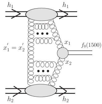
Figure 1: The sketch of the bare QCD mechanism for diffractive production of the glueball. The kinematical variables are shown in addition.

At lower energies ($\sqrt{s}<$ 20 GeV) other processes may become important as well. Since the two-pion channel is one of the dominant decay channels of $f_{0}(1500)$ (34.9 $\pm$ 2.3 %) PDG one may expect the two-pion fusion (see Fig.2 to be one of the dominant mechanisms of exclusive $f_{0}(1500)$ production at the FAIR energies. The two-pion fusion can be also relative reliably calculated in the framework of meson exchange theory. The pion coupling to the nucleon is well known Ericson-Weise . The $\pi NN$ form factor for larger pion virtualities is somewhat less known. This may limit our predictions close to the threshold, where rather large virtualities are involved due to specific kinematics. At largest HESR (antiproton ring) energy, as will be discussed in the present paper, this is no longer a limiting factor as average pion virtualities are rather small.

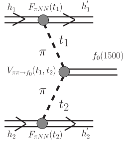
Figure 2: The sketch of the pion-pion MEC mechanism. Form factors appearing in different vertices and kinematical variables are shown explicitly.

II Exclusive processes

II.1 Cross section and phase space

The cross section for a general 3-body reaction $pp\to ppf_{0}(1500)$ can be written as

$$d\sigma_{pp\to ppM}=\frac{1}{2\sqrt{s(s-4m^{2})}}\,\overline{|{\cal M}|^{2}}\cdot d^{\,3}PS\,.$$ (3)

Above $m$ is the mass of the nucleon.

The three-body phase space volume element reads

$$d^{3}PS=\frac{d^{3}p_{1}^{\prime}}{2E_{1}^{\prime}(2\pi)^{3}}\frac{d^{3}p_{2}^{\prime}}{2E_{2}^{\prime}(2\pi)^{3}}\frac{d^{3}P_{M}}{2E_{M}(2\pi)^{3}}\cdot(2\pi)^{4}\delta^{4}(p_{1}+p_{2}-p_{1}^{\prime}-p_{2}^{\prime}-P_{M})\;.$$ (4)

At high energies and small momentum transfers the phase space volume element can be written as KMV99

$$d^{3}PS\approx\frac{1}{2^{8}\pi^{4}}dt_{1}dt_{2}d\xi_{1}d\xi_{2}d\phi\;\delta\left(s(1-\xi_{1})(1-\xi_{2})-M^{2}\right)\;,$$ (5)

where $\xi_{1}$, $\xi_{2}$ are longitudinal momentum fractions carried by outgoing protons with respect to their parent protons and the relative angle between outgoing protons $\Phi\in(0,2\pi)$. Changing variables $(\xi_{1},\xi_{2})\to(x_{F},M^{2})$ one gets

$$d^{3}PS\approx\frac{1}{2^{8}\pi^{4}}dt_{1}dt_{2}\frac{dx_{F}}{s\sqrt{x_{F}^{2}+4(M^{2}+|{\bf P}_{M,t}|^{2})/s}}\;d\Phi\;.$$ (6)

The high-energy formulas (5) and (6) break close to the meson production threshold. Then exact phase space formula (4) must be taken and another choice of variables is more appropriate. We choose transverse momenta of the outgoing nucleons ($p^{\prime}_{1t},p^{\prime}_{2t}$), azimuthal angle between outgoing nucleons ($\phi$) and rapidity of the meson (y) as independent kinematically complete variables. Then the cross section can be calculated as:

$$d\sigma=\sum_{k}{\cal J}^{-1}(p_{1t},p_{2t},\phi,y)|_{k}\frac{\overline{|{\cal M}(p_{1t},p_{2t},\phi,y)|^{2}}}{2\sqrt{s(s-4m^{2})}}\;\frac{2\pi}{(2\pi)^{5}}\frac{1}{2E^{\prime}_{1}}\frac{1}{2E^{\prime}_{2}}\frac{1}{2}\;p_{1t}p_{2t}dp_{1t}dp_{2t}d\phi dy\;,$$ (7)

where $k$ denotes symbolically discrete solutions of the set of equations for $p^{\prime}_{1z}$ and $p^{\prime}_{2z}$:

$$\left\{\begin{array}[]{rcl}\sqrt{s}-E_{M}&=&\sqrt{m_{1t}^{2}+p_{1z}^{{}^{\prime}2}}+\sqrt{m_{2t}^{2}+p_{2z}^{{}^{\prime}2}}\;,\\ -p_{Mz}&=&p^{\prime}_{1z}+p^{\prime}_{2z}\;,\end{array}\right.$$ (10)

where $m_{1t}$ and $m_{2t}$ are transverse masses of outgoing nucleons. The solutions of Eq.(10) depend on the values of integration variables: $p^{\prime}_{1z}=p^{\prime}_{1z}(p^{\prime}_{1t},p^{\prime}_{2t},\phi,y)$ and $p^{\prime}_{2z}=p^{\prime}_{2z}(p^{\prime}_{1t},p^{\prime}_{2t},\phi,y)$. The extra jacobian reads:

$${\cal J}_{k}=\left|\frac{p^{\prime}_{1z}(k)}{\sqrt{m_{1t}^{2}+p^{\prime}_{1z}(k)^{2}}}-\frac{p^{\prime}_{2z}(k)}{\sqrt{m_{2t}^{2}+p^{\prime}_{2z}(k)^{2}}}\right|\;.$$ (11)

In the limit of high energies and central production, i.e. $p^{\prime}_{1z}\gg$ 0 (very forward nucleon1), $-p^{\prime}_{2z}\gg$ 0 (very backward nucleon2) the jacobian becomes a constant ${\cal J}\to\tfrac{1}{2}$.

The matrix element depends on the process and is a function of kinematical variables. The mechanism of the exclusive production of $f_{0}(1500)$ close to the threshold is not known. We shall address this issue here. Therefore different mechanisms will be considered and the corresponding cross sections will be calculated.

II.2 Diffractive QCD amplitude

According to Khoze-Martin-Ryskin approach (KMR) KMR , we write the amplitude of exclusive double diffractive colour singlet production $pp\to ppf_{0}(1500)$ as

$${\cal M}^{g^{*}g^{*}}=\frac{s}{2}\cdot\pi^{2}\frac{1}{2}\frac{\delta_{c_{1}c_{2}}}{N_{c}^{2}-1}\,\Im\int d^{2}q_{0,t}V^{c_{1}c_{2}}_{J}\frac{f^{off}_{g,1}(x_{1},x_{1}^{\prime},q_{0,t}^{2},q_{1,t}^{2},t_{1})f^{off}_{g,2}(x_{2},x_{2}^{\prime},q_{0,t}^{2},q_{2,t}^{2},t_{2})}{q_{0,t}^{2}\,q_{1,t}^{2}\,q_{2,t}^{2}}.$$ (12)

The normalization of this amplitude differs from the KMR one KMR by the factor $s/2$ and coincides with the normalization in our previous work on exclusive $\eta^{\prime}$-production SPT07 . The amplitude is averaged over the colour indices and over two transverse polarisations of the incoming gluons KMR . The bare amplitude above is subjected to absorption corrections which depend on collision energy (the bigger the energy, the bigger the absorption corrections). We shall discuss this issue shortly when presenting our results.

The vertex factor $V_{J}^{c_{1}c_{2}}=V_{J}^{c_{1}c_{2}}(q_{1,t}^{2},q_{2,t}^{2},P_{Mt}^{2})$ in expression (12) describes the coupling of two virtual gluons to $f_{0}(1500)$ meson. Recently the vertex was obtained for off-shell values of $q_{1,t}$ and $q_{2,t}$ in the case of $\chi_{c}(0)$ exclusive production PST07 . An almost alternative way to describe the vertex is to express it via partial decay width $\Gamma(M\to gg)$. The latter (approximate) method can be used also for glueball production.

In the original Khoze-Martin-Ryskin (KMR) approach KMR the amplitude is written as

$${\cal M}=N\int\frac{d^{2}q_{0,t}P[f_{0}(1500)]}{q_{0,t}^{2}q_{1,t}^{2}q_{2,t}^{2}}f_{g}^{KMR}(x_{1},x^{\prime}_{1},Q_{1,t}^{2},\mu^{2};t_{1})f_{g}^{KMR}(x_{2},x^{\prime}_{2},Q_{2,t}^{2},\mu^{2};t_{2})\;,$$ (13)

where only one transverse momentum is taken into account somewhat arbitrarily as

$$Q_{1,t}^{2}=\mathrm{min}\{q_{0,t}^{2},q_{1,t}^{2}\}\;,\qquad Q_{2,t}^{2}=\mathrm{min}\{q_{0,t}^{2},q_{2,t}^{2}\}\;,$$ (14)

and the normalization factor $N$ can be written in terms of the $f_{0}(1500)\to gg$ decay width (see below).

In the KMR approach the large meson mass approximation $M\gg|{\bf q}_{1,t}|,\,|{\bf q}_{2,t}|$ is adopted, so the gluon virtualities are neglected in the vertex factor

$$P[f_{0}(1500)]\simeq(q_{1,t}q_{2,t})=(q_{0,t}+p^{\prime}_{1,t})(q_{0,t}-p^{\prime}_{2,t}).$$ (15)

The KMR UGDFs are written in the factorized form:

$$f_{g}^{KMR}(x,x^{\prime},Q_{t}^{2},\mu^{2};t)=f_{g}^{KMR}(x,x^{\prime},Q_{t}^{2},\mu^{2})\exp(b_{0}t)$$ (16)

with $b_{0}=2$ GeV^-2 KMR . In our approach we use somewhat different parametrization of the $t$-dependent isoscalar form factors.

Please note that the KMR and our (general) skewed UGDFs have different number of arguments. In the KMR approach there is only one effective gluon transverse momentum (see Eq.(14)) compared to two idependent transverse momenta in general case (see Eq.(20)).

The KMR skewed distributions are given in terms of conventional integrated densities $g$ and the so-called Sudakov form factor $T$ as follows:

$$f_{g}^{KMR}(x,x^{\prime},Q_{t}^{2},\mu^{2})=R_{g}\frac{\partial}{\partial\ln Q_{t}^{2}}\left[\sqrt{T(Q_{t}^{2},\mu^{2})}xg(x,Q_{t}^{2})\right]\;.$$ (17)

The square root here was taken using arguments that only survival probability for hard gluons is relevant. It is not so-obvious if this approximation is reliable for light meson production. The factor $R_{g}$ in the KMR approach approximately accounts for the single $\log Q^{2}$ skewed effect KMR . Please note also that in contrast to our approach the skewed KMR UGDF does not explicitly depend on $x^{\prime}$ (assuming $x^{\prime}\ll x\ll 1$). Usually this factor is estimated to be 1.3–1.5. In our evaluations here we take it to be equal 1 to avoid further uncertainties. Following now the KMR notations we write the total amplitude (12) (averaged over colour and polarisation states of incoming gluons) in the limit $M\gg q_{1,t},\,q_{2,t}$ as

$${\cal M}=A\,\pi^{2}\,\frac{s}{2}\,\int d^{2}q_{0,t}P[f_{0}(1500)]\frac{f^{off}_{g,1}(x_{1},x_{1}^{\prime},q_{0,t}^{2},q_{1,t}^{2},t_{1})f^{off}_{g,2}(x_{2},x_{2}^{\prime},q_{0,t}^{2},q_{2,t}^{2},t_{2})}{q_{0,t}^{2}\,q_{1,t}^{2}\,q_{2,t}^{2}}\,,$$ (18)

where the normalization constant is

$$A^{2}=\frac{64\pi\Gamma(f_{0}(1500)\rightarrow gg)}{(N_{c}^{2}-1)M^{3}}\;.$$ (19)

In addition to the standard KMR approach we could use other off-diagonal distributions (for details and a discussion see SPT07 ; PST07 ). In the present work we shall use a few sets of unintegrated gluon distributions which aim at the description of phenomena where small gluon transverse momenta are involved. Some details concerning the distributions can be found in Ref. LS06 . We shall follow the notation there.

In the general case we do not know off-diagonal UGDFs very well. In SPT07 ; PST07 we have proposed a prescription how to calculate the off-diagonal UGDFs:

$$f_{g,1}^{off} = \sqrt{f_{g}^{(1)}(x_{1}^{\prime},q_{0,t}^{2},\mu_{0}^{2})\cdot f_{g}^{(1)}(x_{1},q_{1,t}^{2},\mu^{2})}\cdot F_{1}(t_{1})\,,$$

$$f_{g,2}^{off} = \sqrt{f_{g}^{(2)}(x_{2}^{\prime},q_{0,t}^{2},\mu_{0}^{2})\cdot f_{g}^{(2)}(x_{2},q_{2,t}^{2},\mu^{2})}\cdot F_{1}(t_{2})\,,$$ (20)

where $F_{1}(t_{1})$ and $F_{1}(t_{2})$ are isoscalar nucleon form factors. They can be parametrized as (PST07 )

$$F_{1}(t_{1,2})=\frac{4m_{p}^{2}-2.79\,t_{1,2}}{(4m_{p}^{2}-t_{1,2})(1-t_{1,2}/071)^{2}}\;.$$ (21)

Above $t_{1}$ and $t_{2}$ are total four-momentum transfers in the first and second proton line, respectively. While in the emission line the choice of the scale is rather natural, there is no so-clear situation for the second screening-gluon exchange SPT07 .

Even at intermediate energies ($W$ = 10-50 GeV) typical $x_{1}^{{}^{\prime}}=x_{2}^{{}^{\prime}}$ are relatively small ($\sim$ 0.01). However, characteristic $x_{1},x_{2}\sim M_{f_{0}}/\sqrt{s}$ are not too small (typically $>$ 10^-1). Therefore here we cannot use the small-$x$ models of UGDFs. In the latter case a Gaussian smearing of the collinear distribution seems a reasonable solution:

$${\cal F}_{g}^{Gauss}(x,k_{t}^{2},\mu_{F}^{2})=xg^{coll}(x,\mu_{F}^{2})\cdot f_{Gauss}(k_{t}^{2};\sigma_{0})\;,$$ (22)

where $g^{coll}(x,\mu_{F}^{2})$ are standard collinear (integrated) gluon distribution and $f_{Gauss}(k_{t}^{2};\sigma_{0})$ is a Gaussian two-dimensional function

$$\begin{split}f_{Gauss}(k_{t}^{2},\sigma_{0})=\frac{1}{2\pi\sigma_{0}^{2}}\exp\left(-k_{t}^{2}/2\sigma_{0}^{2}\right)/\pi\,.\end{split}$$ (23)

Above $\sigma_{0}$ is a free parameter which one can expect to be of the order of 1 GeV. Based on our experience in SPT07 we expect strong sensitivity to the actual value of the parameter $\sigma_{0}$. Summarizing, a following prescription for the off-diagonal UGDF seems reasonable:

$$f(x,x^{\prime},k_{t}^{2},k_{t}^{{}^{\prime}2},t)=\sqrt{f_{small-x}(x^{\prime},k_{t}^{{}^{\prime}2})f_{Gauss}(x,k_{t}^{2},\mu^{2})}\cdot F(t)\;,$$ (24)

where $f_{small-x}(x^{\prime},k_{t}^{{}^{\prime}2})$ is one of the typical small-$x$ UGDFs (see e.g.LS06 ). So exemplary combinations are: KL $\otimes$ Gauss, BFKL $\otimes$ Gauss, GBW $\otimes$ Gauss (for notation see LS06 ). The natural choice of the scale is $\mu^{2}=M_{f_{0}}^{2}$. This relatively low scale is possible with the GRV-type of PDF parametrization GRV . We shall call (24) a ”mixed prescription” for brevity.

II.3 Two-gluon impact factor approach for subasymptotic energies

The amplitude in the previous section, written in terms of off-diagonal UGDFs, was constructed for large energies. The smaller the energy the shorter the QCD ladder. It is not obvious how to extrapolate the diffractive amplitude down to lower (close-to-threshold) energies. Here we present slightly different method which seems more adequate at lower energies.

At not too large energies the amplitude of elastic scattering can be written as amplitude for two-gluon exchange pp_elastic_2g_if ; SNS02

$${\cal M}_{pp\to pp}(s,t)=is\frac{N_{c}^{2}-1}{N_{c}^{2}}\int d^{2}k_{t}\;\alpha_{s}(k_{1t}^{2})\alpha_{s}(k_{2t}^{2})\frac{3F({\bf k}_{1t},{\bf k}_{2t})3F({\bf k}_{1t},{\bf k}_{2t})}{(k_{1t}^{2}+\mu_{g}^{2})(k_{2t}^{2}+\mu_{g}^{2})}\;.$$ (25)

In analogy to dipole-dipole or pion-pion scattering (see e.g. SNS02 ) the impact factor can be parametrized as:

$$F({\bf k}_{1t},{\bf k}_{2t})=\frac{A^{2}}{A^{2}+({\bf k}_{1t}+{\bf k}_{2t})^{2}}-\frac{A^{2}}{A^{2}+({\bf k}_{1t}-{\bf k}_{2t})^{2}}\;.$$ (26)

At high energy the net four-momentum transfer: $t=-({\bf k}_{1t}+{\bf k}_{2t})^{2}$. $A$ in Eq.(25) is a free parameter which can be adjusted to elastic scattering. For our rough estimate we take $A=m_{\rho}$.

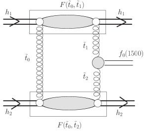
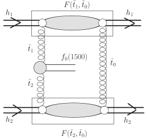
Figure 3: The sketch of the two-gluon impact factor approach. Some kinematical variables are shown explicitly.

Generalizing, the amplitude for exclusive $f_{0}(1500)$ production can be written as the amplitude for three-gluon exchange shown in Fig.3:

$${\cal M}_{pp\to ppf_{0}(1500)}(s,y,t_{1},t_{2},\phi)=is\frac{N_{c}^{2}-1}{N_{c}^{2}}\int d^{2}k_{0t}$$

$$\left(\alpha_{s}(k_{0t}^{2})\alpha_{s}(k_{1t}^{2})\right)^{1/2}\left(\alpha_{s}(k_{0t}^{2})\alpha_{s}(k_{2t}^{2})\right)^{1/2}$$

$$\frac{3F({\bf k}_{0t},{\bf k}_{1t})3F({\bf k}_{0t},{\bf k}_{2t})}{(k_{0t}^{2}+\mu_{g}^{2})(k_{1t}^{2}+\mu_{g}^{2})(k_{2t}^{2}+\mu_{g}^{2})}\;V_{gg\to f_{0}(1500)}({\bf k}_{1t},{\bf k}_{2t})\;.$$ (27)

At high energy and $y\approx$ 0 the four-momentum transfers can be calculated as:
$t_{1}=-({\bf k}_{0t}+{\bf k}_{1t})^{2}$, $t_{2}=-({\bf k}_{0t}-{\bf k}_{2t})^{2}$.
At low energy and/or $y\neq$ 0 the kinematics is slightly more complicated. Let us define effective four-vector transfers:

$$q_{1} = (p^{\prime}_{1}-p_{1})=(q_{10},q_{1x},q_{1y},q_{1z})\;,$$

$$q_{2} = (p^{\prime}_{2}-p_{2})=(q_{20},q_{2x},q_{2y},q_{2z})\;.$$ (28)

Then $t_{1}\equiv q_{1}^{2}=q_{1l}^{2}+q_{1t}^{2}$ and $t_{2}\equiv q_{2}^{2}=q_{2l}^{2}+q_{2t}^{2}$. Close to threshold the longitudinal components $q_{1l}^{2}=q_{10}^{2}-q_{1z}^{2}\ll$ 0 and $q_{2l}^{2}=q_{20}^{2}-q_{2z}^{2}\ll$ 0. Then the amplitude (27) must be corrected. Then also four-vectors of exchanged gluons ($k_{0}$, $k_{1}$ and $k_{2}$) cannot be purely transverse and longitudinal components must be included as well. To estimate the effect we use formula (27) but modify the transferred four momenta of gluons entering the $g^{*}g^{*}\to f_{0}(1500)$ production vertex:

$$k_{1} = (0,{\bf k}_{1t},0)\to(q_{10},{\bf k}_{1t},q_{1z})\;,$$

$$k_{2} = (0,{\bf k}_{2t},0)\to(q_{20},{\bf k}_{2t},q_{2z})\;$$ (29)

and leave $k_{0}$ purely transverse. This procedure is a bit arbitrary but comparing results obtained with formula (27) with that from the formula with modified four-momenta would allow to estimate related uncertainties.

We write the vertex function $gg\to f_{0}(1500)$ in the following tensorial form :

$$V(k_{1},k_{2},p_{M})=C_{f_{0}(1500)\to gg}\;g_{\mu\nu}k_{1}^{\mu}k_{2}^{\nu}\;.$$ (30)

The normalization factor is obtained from the decay of $f_{0}(1500)$ into two soft gluons:

$$|C_{f_{0}(1500)\to gg}|^{2}=\frac{64\pi}{M_{f_{0}}^{3}(N_{c}^{2}-1)}\Gamma_{f_{0}(1500)\to gg}\;.$$ (31)

Of course the partial decay width is limited from above:

$$\Gamma_{f_{0}(1500)\to gg}<\Gamma_{tot}\;.$$ (32)

The amplitudes discussed here involve transverse momenta in the infra-red region. Then a prescription how to extend the perturbative $\alpha_{s}(k_{t}^{2})$ dependence to a nonperturbative region of small gluon virtualities is unavoidable. In the following $\alpha_{s}(k_{t}^{2})$ is obtained from an analytic freezing proposed by Shirkov and Solovtsev SS97 .

II.4 Pion-pion MEC amplitude

It is straightforward to evaluate the pion-pion meson exchange current contribution shown in Fig.2. If we assume the $i\gamma_{5}$ type coupling of the pion to the nucleon then the Born amplitude reads:

$$\overline{|{\cal M}|^{2}}=\frac{1}{4} [\left(E_{1}+m\right)\left(E_{1}^{\prime}+m\right)\left(\frac{{\bf p}_{1}^{2}}{(E_{1}+m)^{2}}+\frac{{\bf p}_{1}^{{}^{\prime}2}}{(E_{1}^{{}^{\prime}}+m)^{2}}-\frac{2{\bf p}_{1}\cdot{\bf p}^{{}^{\prime}}_{1}}{(E_{1}+m)(E_{1}^{{}^{\prime}}+m)}\right)]\cdot 2$$

$$\frac{g_{\pi NN}^{2}\;\cdot T_{k}}{(t_{1}-m_{\pi}^{2})^{2}}F_{\pi NN}^{2}(t_{1})\;\cdot\;|C_{f_{0}(1500)\to\pi\pi}|^{2}\;V_{\pi\pi\to f_{0}(1500)}^{2}(t_{1},t_{2})\;\cdot\;\frac{g_{\pi NN}^{2}\;\cdot T_{k}}{(t_{2}-m_{\pi}^{2})^{2}}F_{\pi NN}^{2}(t_{2})$$

$$[\left(E_{2}+m\right)\left(E_{2}^{\prime}+m\right)\left(\frac{{\bf p}_{2}^{2}}{(E_{2}+m)^{2}}+\frac{{\bf p}_{2}^{{}^{\prime}2}}{(E_{2}^{{}^{\prime}}+m)^{2}}-\frac{2{\bf p}_{2}\cdot{\bf p}^{{}^{\prime}}_{2}}{(E_{2}+m)(E_{2}^{{}^{\prime}}+m)}\right)]\cdot 2\;$$

. (33)

In the formula above $m$ is the mass of the nucleon, $E_{1},E_{2}$ and $E_{1}^{\prime},E_{2}^{\prime}$ are energies of initial and outgoing nucleons, ${\bf p}_{1},{\bf p}_{2}$ and ${\bf p}^{\prime}_{1},{\bf p}^{\prime}_{2}$ are corresponding three-momenta and $m_{\pi}$ is the pion mass. The factor $g_{\pi NN}$ is the familiar pion nucleon coupling constant which is precisely known ($\frac{g_{\pi NN}^{2}}{4\pi}$ = 13.5 – 14.6). The isospin factor $T_{k}$ equals 1 for the $\pi^{0}\pi^{0}$ fusion and equals 2 for the $\pi^{+}\pi^{-}$ fusion. In the case of proton-proton collisions only the $\pi^{0}\pi^{0}$ fusion is allowed while in the case of proton-antiproton collisions both $\pi^{0}\pi^{0}$ and $\pi^{+}\pi^{-}$ MEC are possible. In the case of central heavy meson production rather large transverse momenta squared $t_{1}$ and $t_{2}$ are involved and one has to include extended nature of the particles involved in corresponding vertices. This is incorporated via $F_{\pi NN}(t_{1})$ or $F_{\pi NN}(t_{2})$ vertex form factors. The influence of the t-dependence of the form factors will be discussed in the result section. In the meson exchange approach MHE87 they are parametrized in the monopole form as

$$F_{\pi NN}(t)=\frac{\Lambda^{2}-m_{\pi}^{2}}{\Lambda^{2}-t}\;.$$ (34)

A typical values are $\Lambda$ = 1.2–1.4 GeV MHE87 . The Gottfried Sum Rule violation prefers smaller $\Lambda\approx$ 0.8 GeV GSR .

The normalization constant $|C|^{2}$ in (33) can be calculated from the partial decay width as

$$|C_{f_{0}(1500)\to\pi\pi}|^{2}=\frac{8\pi\;2M_{f_{0}}^{2}\Gamma_{f_{0}(1500)\to\pi^{0}\pi^{0}}}{\sqrt{M_{f_{0}}^{2}-4m_{\pi}^{2}}}\;,$$ (35)

where $\Gamma_{f_{0}(1500)\to\pi^{0}\pi^{0}}=0.109\cdot BR(f_{0}(1500)\to\pi\pi)\cdot 0.5$ GeV. The branching ratio is $BR(f_{0}(1500)\to\pi\pi)$ = 0.349 PDG . The off-shellness of pions is also included for the $\pi\pi\to f_{0}(1500)$ transition through the extra $V_{\pi\pi\to f_{0}(1500)}(t_{1},t_{2})$ form factor which we take in the factorized form:

$$V_{\pi\pi\to f_{0}(1500)}(t_{1},t_{2})=\frac{\Lambda_{\pi\pi f_{0}}^{2}-m_{\pi}^{2}}{\Lambda_{\pi\pi f_{0}}^{2}-t_{1}}\cdot\frac{\Lambda_{\pi\pi f_{0}}^{2}-m_{\pi}^{2}}{\Lambda_{\pi\pi f_{0}}^{2}-t_{2}}\;.$$ (36)

It is normalized to unity when both pions are on mass shell

$$V(t_{1}=m_{\pi}^{2},t_{2}=m_{\pi}^{2})=1\;.$$ (37)

In the present calculation we shall take $\Lambda_{\pi\pi f_{0}}$ = 1.0 GeV.

III Results

III.1 Gluonic QCD mechanisms

Let us start with the QCD mechanism relevant at higher energies. We wish to present differential distributions in $x_{F}$, $t_{1}$ or $t_{2}$ and relative azimuthal angle $\phi$. In the following we shall assume: $\Gamma_{f_{0}(1500)\to gg}=\Gamma_{f_{0}(1500)}^{tot}$ . This assumption means that our differential distributions mean upper value of the cross section. If the fractional branching ratio is known, our results should be multiplied by its value.

In Fig.4 we show as example distribution in Feynman $x_{F}$ for Kharzeev-Levin UGDF (solid) and the mixed distribution KL $\otimes$ Gaussian (dashed) for several values of collision energy in the interval $W$ = 10 – 50 GeV. In general, the higher collision energy the larger cross section. With the rise of the initial energy the cross section becomes peaked more and more at $x_{F}\sim$ 0. The mixed UGDF produces slightly broader distribution in $x_{F}$.

Figure 4: The distribution of $f_{0}(1500)$ in Feynman $x_{F}$ for W = 10, 20, 30, 40, 50 GeV. In this calculation the Kharzeev-Levin UGDF (solid line) and the mixed distribution KL$\otimes$ Gauss (dashed line) were used.

In Fig.5 we present corresponding distributions in $t=t_{1}=t_{2}$. The slope depends on UGDF used, but for a given UGDF is almost energy independent.

Figure 5: Distribution in $t=t_{1}=t_{2}$ for Kharzeev-Levin UGDF for $W=$ 10, 20, 30, 40, 50 GeV. The notation here is the same as in Fig.4.

Finally we present corresponding distributions in relative azimuthal angle between outgoing protons or proton and antiproton . These distributions have maximum when outgoing nucleons are back-to-back. Again the shape seems to be only weekly energy dependent.

Figure 6: Distribution in relative azimuthal angle for different UGDFs for $W$ = 10, 20, 30, 40, 50 GeV. The notation here is the same as in Fig.4.

III.2 Gluonic versus pion-pion mechanism

What about the pion-pion fusion mechanism? Can it dominate over the gluonic mechanism discussed in the previous subsection? In Fig.7 we show the integrated cross section for the exclusive $f_{0}(1500)$ elastic production

$$p\bar{p}\to pf_{0}(1500)\bar{p}$$ (38)

and for double charge exchange reaction

$$p\bar{p}\to nf_{0}(1500)\bar{n}\;.$$ (39)

The thick solid line represents the pion-pion component calculated with monopole vertex form factors (34) with $\Lambda$ = 0.8 GeV (lower) and $\Lambda$ = 1.2 GeV (upper). The difference between the lower and upper curves represents uncertainties on the pion-pion compenent. The pion-pion contribution grows quickly from the threshold, takes maximum at $W\approx$ 6-7 GeV and then slowly drops with increasing energy. The gluonic contribution calculated with unintegrated gluon distributions drops with decreasing energy towards the kinematical threshold and seems to be about order of magnitude smaller than the pion-pion component at W = 10 GeV. We show the result with Kharzeev-Levin UGDF (dashed line) which includes gluon saturation effects relevant for small-x, Kimber-Martin-Ryskin UGDF (dotted line) used for the exclusive production of the Higgs boson and the result with the ”mixed prescription” (KL $\otimes$ Gaussian) for different values of the $\sigma_{0}$ parameter: 0.5 GeV (upper thin solid line), 1.0 GeV (lower thin solid line). In the latter case results rather strongly depend on the value of the smearing parameter.

We calculate the gluonic contribution down to W = 10 GeV. Extrapolating the gluonic component to even lower energies in terms of UGDFs seems rather unsure. At lower energies the two-gluon impact factor approach seems more relevant. The impact factor approach result is even order of magnitude smaller than that calculated in the KMR approach (see lowest dash-dotted (red on-line) line in Fig. 7), so it seems that the diffractive contribution is rather negligible at the FAIR energies.

Our calculation suggests that quite different energy dependence of the cross section may be expected in elastic and charge-exchange channels. Experimental studies at FAIR and J-PARC could shed more light on the glueball production mechanism.

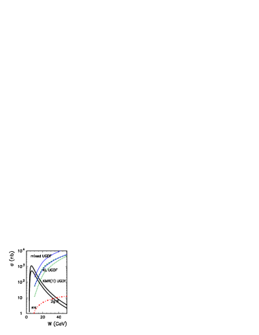
Figure 7: The integrated cross section as a function of the center of mass energy for $p\bar{p}\to p\bar{p}f_{0}(1500)$ (left panel) and $p\bar{p}\to n\bar{n}f_{0}(1500)$ (right panel) reactions. The thick solid lines are for pion-pion MEC contribution ($\Lambda$ = 0.8, 1.2 GeV), the dashed line is for QCD diffractive contribution obtained with the Kharzeev-Levin UGDF, the dotted line for the KMR approach and the thin solid lines (blue on-line) are for ”mixed” UGDF (KL $\otimes$ Gaussian) with $\sigma_{0}$ = 0.5, 1 GeV. The dash-dotted line represents the two-gluon impact factor result.

III.3 Predictions for PANDA at HESR

Let us concentrate now on $p\bar{p}$ collisions at energies relevant for future experiments at HESR at the FAIR facilite in GSI. Here the pion-pion MEC (see Fig.2) seems to be the dominant mechanism, especially for the charge exchange reaction $p\bar{p}\to n\bar{n}f_{0}(1500)$.

In Fig.8 we show average values of $t_{1}$ (or $t_{2}$) for the two-pion MEC as a function of the center of mass energy. Close to threshold $W=2m_{N}+m_{f_{0}(1500)}$ the transferred four-momenta squared are the biggest, of the order of about 1.5 GeV². The bigger energy the smaller the transferred four-momenta squared. Therefore experiments close to threshold open a unique possibility to study physics of large transferred four-momenta squared at relatively small energies. This is a quite new region, which was not studied so far in the literature.

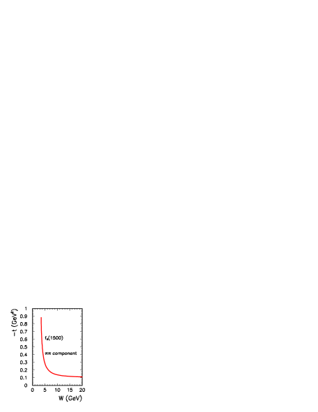
Figure 8: Average value of $<t_{1}>=<t_{2}>$ as a function of the center-of-mass collision energy for the two-pion exchange mechanism.

The maximal energy planned for HESR is $\sqrt{s}$ = 5.5 GeV. At this energy the phase space is still very limited. In Fig.9 we show rapidity distribution of $f_{0}(1500)$. For comparison the rapidity of incoming antiproton and proton is 1.72 and -1.72, respectively. This means that in the center-of-mass system the glueball is produced at midrapidities, on average between rapidities of outgoing nucleons.

Figure 9: rapidity distribution of $f_{0}(1500)$ produced in the reaction $p\bar{p}\to n\bar{n}f_{0}(1500)$ for W = 3.5, 4.0, 4.5, 5.0, 5.5 GeV (maximal HESR energy). In this calculation $\Lambda$ = 0.8 GeV.

In Fig.10 we show transverse momentum distribution of neutrons or antineutrons produced in the reaction $p\bar{p}\to n\bar{n}f_{0}(1500)$. The distribution depends on the $\pi NN$ form factors $F_{\pi NN}(t_{1})$ and $F_{\pi NN}(t_{2})$ in formula (33).

Figure 10: Transverse momentum distribution of neutrons or antineutrons produced in the reaction $p\bar{p}\to n\bar{n}f_{0}(1500)$ for W = 3.5, 4.0, 4.5, 5.0, 5.5 GeV (maximal HESR energy). In this calculation $\Lambda$ = 0.8 GeV.

In Fig.11 we show azimuthal angle correlation between outgoing hadrons (in this case neutron and antineutron). The preference for back-to-back configurations is caused merely by the limitations of the phase space close to the threshold. This correlation vanishes in the limit of infinite energy. In practice far from the threshold the distribution becomes almost constant in azimuth. This has to be contrasted with similar distributions for pomeron-pomeron fusion shown in Fig.6 which are clearly peaked for the back-to-back configurations. Therefore a deviation from the constant distribution in relative azimuthal angle for the highest HESR energy of W = 5.5 GeV for $p\bar{p}\to pf_{0}(1500)\bar{p}$ can be a signal of the gluon induced processes. It is not well understood what happens with the gluon induced diffractive processes when going down to intermediate (W = 5-10 GeV) energies. A future experiment performed by the PANDA collaboration could bring new insights into this issue. This would be also a signal that the $f_{0}(1500)$ state has a considerable glueball component.

Figure 11: Azimuthal angle correlations between neutron and antineutron produced in the reaction $p\bar{p}\to n\bar{n}f_{0}(1500)$ for W = 3.5, 4.0, 4.5, 5.0, 5.5 GeV (maximal HESR energy). In this calculation $\Lambda$ = 0.8 GeV.

Up to now we have neglected interference between pion-pion and pomeron-pomeron contributions (for the same final channel). This effect may be potentially important when both components are of the same order of magnitude. While the pomeron-pomeron contribution is dominantly nucleon helicity preserving the situation for pion-pion fusion is more complicated. In the latter case we define 4 classes of contributions with respect to the nucleon helicities: $cc$ (both helicity conserved), $cf$ (first conserved, second flipped), $fc$ (first flipped, second conserved) and $ff$ (both helicities flipped). The corresponding ratios of individual contributions to the sum of all contributions are shown in Fig.12. In practice, only the $cc$ $\pi\pi$ contribution may potentially interfere with the gluonic one. From the figure one can conclude that this can happen only when both transverse momenta of the final nucleons are small. We shall leave numerical studies of the interference effect for future investigations, when experimental details of such measurements will be better known; but already now one can expect them to be rather small.

Figure 12: Helicity decomposition of the cross section on the ($p_{1t},p_{2t}$) plane for W = 10 GeV. $R_{cc}$ (upper left), $R_{ff}$ (upper right), $R_{cf}$ (lower left), $R_{fc}$ (lower right). The standard nucleon dipole form factor was used in this calculation.

IV Discussion and Conclusions

We have estimated the cross section for exclusive $f_{0}(1500)$ production not far from the threshold. We have included both gluon induced diffractive mechanism and the pion-pion exchange contributions. The first was obtained by extrapolating down the cross section in the Khoze-Martin-Ryskin approach with unintegrated gluon distributions from the literature as well as using two-gluon impact factor approach. A rather large uncertainties are associated with the diffractive component. The calculation of MEC contribution requires introducing extra vertex form factors which are not extremely well constraint. This is especially important close to the threshold where rather large $|t_{1}|$ and $|t_{2}|$ are involved. The cross section for energies close to the threshold is very sensitive to the functional form and parameters of vertex form factor. Therefore a measurement of $f_{0}(1500)$ close to its production threshold could limit the so-called $\pi NN$ form factors in the region of exchanged four-momenta never tested before.

We predict the dominance of the pion-pion contribution close to the threshold and diffractive component far from the threshold. Taking into account rather large uncertainties these predictions should be taken with some grain of salt. Clearly an experimental program is required to disantagle the reaction mechanism.

Disantangling the mechanism of the exclusive $f_{0}(1500)$ production not far from the meson production threshold would require study of the $p\bar{p}\to p\bar{p}f_{0}(1500)$, $p\bar{p}\to n\bar{n}f_{0}(1500)$ processes with PANDA detector at FAIR and $pp\to ppf_{0}(1500)$ reaction at J-PARC. In the case the gluonic mechanisms are small and the pion exchange mechanism is a dominant process one expects: $\sigma(p\bar{p}\to n\bar{n}f_{0}(1500))=4\times\sigma(p\bar{p}\to p\bar{p}f_{0}(1500))$. On the other hand if the gluonic components dominate over MEC components $\sigma(p\bar{p}\to p\bar{p}f_{0}(1500))>\sigma(p\bar{p}\to n\bar{n}f_{0}(1500))$.

Therefore a careful studies of different final channels at FAIR and J-PARC could help to shed light on coupling of (nonperturbative) gluons to $f_{0}(1500)$ and therefore would give a new hint on its nature. Such studies are not easy at all as in the $\pi\pi$ decay channel one expects a large continuum. This continuum requires a better theoretical estimate. A partial wave $\pi\pi$ analysis may be unavoidable in this context. The two-pion continuum will be studied in our future work. A smaller continuum may be expected in the $K\bar{K}$ or four-pion $f_{0}(1500)$ decay channel. This requires, however, a good geometrical (full solid angle) coverage and high registration efficiencies. PANDA detector seems to fullfil these requirements, but planning real experiment requires a dedicated Monte Carlo simulation of the apparatus.

Acknowledgements We are indebted to Roman Pasechnik, Wolfgang Schäfer and Oleg Teryaev for a discussion and Tomasz Pietrycki for a help in preparing diagrams.

References

-
(1)
C. Amsler et al. (Crystal Barrel Collaboration),
Phys. Lett. B327 425 (1994);
C. Amsler et al. (Crystal Barrel Collaboration), Phys. Lett. B333 277 (1994);
C. Amsler et al. (Crystal Barrel Collaboration), Phys. Lett. B340 259 (1994) - (2) V.V. Anisovich, Phys. Lett. B364 (1995) 195.
- (3) D. Barberis et al. (WA102 Collaboration), Phys. Lett. B462 (1999) 279.
- (4) D. Barberis et al. (WA102 Collaboration), hep-ex/0001017.
-
(5)
C. Amsler and F.E. Close,
Phys. Rev. D53 295 (1996);
F.E. Close, Acta Phys.Polon. B31 2557 (2000). -
(6)
F.E. Close and A. Kirk, Phys. Lett. B397 333 (1997);
F.E. Close and A. Kirk, Phys. Lett. B477 13 (2000). -
(7)
F.E. Close and G.A. Schuler, Phys. Lett. B458 127 (1999);
F.E. Close and G.A. Schuler, Phys. Lett. B464 279 (1999). -
(8)
V.A. Khoze, A.D. Martin and M.G. Ryskin, Phys. Lett. B 401,
330 (1997);
V.A. Khoze, A.D. Martin and M.G. Ryskin, Eur. Phys. J. C 23, 311 (2002);
A.B. Kaidalov, V.A. Khoze, A.D. Martin and M.G. Ryskin, Eur. Phys. J. C 31, 387 (2003) [arXiv:hep-ph/0307064];
A.B. Kaidalov, V.A. Khoze, A.D. Martin and M.G. Ryskin, Eur. Phys. J. C 33, 261 (2004);
V.A. Khoze, A.D. Martin, M.G. Ryskin and W.J. Stirling, Eur. Phys. J. C 35, 211 (2004). - (9) F.E. Close and Q. Zhao, Phys. Rev. D71 (2005) 094022.
- (10) A. Szczurek, R. S. Pasechnik and O. V. Teryaev, Phys. Rev. D 75, 054021 (2007) [arXiv:hep-ph/0608302].
- (11) R. S. Pasechnik, A. Szczurek and O. V. Teryaev, arXiv:0709.0857 [hep-ph], in print in Phys. Rev. D.
- (12) M. Łuszczak and A. Szczurek, Phys. Rev. D73, 054028 (2006).
-
(13)
M. Glück, E. Reya and A. Vogt, Z. Phys. C67, 433 (1995);
M. Glück, E. Reya and A. Vogt, Eur. Phys. J. C5, 461 (1998). - (14) N.I. Kochelev, T. Morii and A.V. Vinnikov, Phys. Lett. B457 (1999) 202.
- (15) T. Ericson and A. Thomas, Pions and Nuclei, Oxford University Press, 1988.
- (16) R. Machleidt, K. Holinde and Ch. Elster, Phys. Rep. 149 (1987) 1.
-
(17)
A. Szczurek and J. Speth, Nucl. Phys. A555 (1993) 249;
B. C. Pearce, J. Speth and A. Szczurek, Phys. Rep. 242 (1994) 193;
J. Speth and A.W. Thomas, Adv. Nucl. Phys. 24 (1997) 83. - (18) F.E. Close, A. Kirk and G. Schuler, hep-ph/0001158.
- (19) D.V. Shirkov and I.L. Solovtsov, Phys. Rev. Lett.79 1209 (1997).
-
(20)
J.F. Gunion and D.E. Soper, Phys. Rev. D15 (1977) 2617;
E.M. Levin and M.G. Ryskin, Sov. J. Nucl. Phys. 34 (1981) 619. - (21) A. Szczurek, N.N. Nikolaev and J. Speth, Phys. Rev. C66 (2002) 055206.
- (22) W. M. Yao et al. (Particle Data Group), Jour. Phys. G33 1 (2006).