Visualization Drivers for Geant4
Fermilab-TM-2329-CD, Oct 2005

Abstract

This document is on Geant4 visualization tools (drivers), evaluating pros and cons of each option, including recommendations on which tools to support at Fermilab for different applicationsDaniel .

Four visualization drivers are evaluated. They are OpenGL, HepRep, DAWN and VRML. They all have good features, OpenGL provides graphic output with out an intermediate file! HepRep provides menus to assist the user. DAWN provides high quality plots and even for large files produces output quickly. VRML uses the smallest disk space for intermediate files.

Large experiments at Fermilab will want to write their own display. They should proceed to make this display graphics independent. Medium experiment will probably want to use HepRep because of it’s menu support. Smaller scale experiments will want to use OpenGL in the spirit of having immediate response, good quality output and keeping things simple.

I Introduction

This report start with the sections Introduction, Documentation, Available Drivers, followed by a tour of Visualization. The tour shows plots produced by Geant4 using four different device drivers. The next section is on Building OpenGL a graphics device driver that produces immediate results. Followed by two further sections on OpenGL. We then treat graphic device drivers that require intermediate files. These are HepRep, DAWN and VRML. An important subsection is ‘Summary of intermediate files’. The report concludes with ‘Which driver to use?’.

Very important to any experiment is a good way to visualize the results.To illustrate this obvious point I have selected an example from High Energy Physics (HEP). I was lucky to be able to play a part in the CDF display CDF_Display . By looking at the central tracking display and seeing that there were very few high P_t tracks in minimum-bias events, it was obvious that a fast trigger processor was needed for the experiment. The central tracking chamber is a cylindrical drift chamber located in a 1.5-T magnetic field provided by a super-conducting solenoid coaxial with the beam. Thus high P_t tracks are almost straight lines. Jim Freeman and Bill Foster proposed and built the first fast trigger processor for the experiment.

Equally true is that any experiment today needs a simulation. The total cross section for $p\overline{p}$ interactions at $\sqrt{s}$ = 1800 GeV was measured by two groups CDF and E811total . One used a simulation(CDF) and one did not(E811). The results differ by about 2.8$\sigma$. I along with some of my CDF collaborators wrote a report that indicated it was much better to have the simulationCDF_E811 .

For any experiment it is always good if you can show a display and histogram for the experiment and the corresponding simulation. The context of different applications is very broad at Fermilab. Clearly the most important item on our agenda is the Linear Collider. Pier Oddone explains this in his “A vision for Fermilab”vision . Physicist at SLAC are already using Geant4 in detector simulations for the Linear Collider. The CMS detector is shown in Fig. 1.

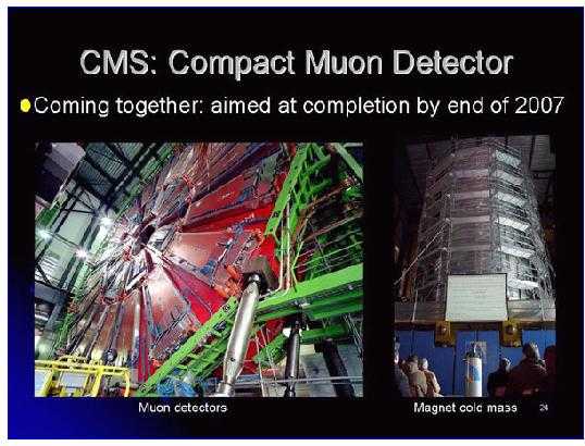
Figure 1: This is slide #24 from the talk by Pier Oddone showing the CMS detector.
The CMS collaboration has 2000 members of which 300 are in the US.

The CMS experiment is currently rewriting it’s softwareEDM . The new software will use Geant4. The older software called OSCAR also uses Geant4OSCAR . Geant4 has also been used to simulate a test of the Hadron Calorimeter which occurred in 2002. Of the current experiments MiniBooNE (see Fig. 2) is using Geant4.

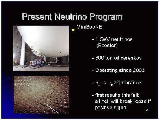
Figure 2: This is slide #29 from the talk by Pier Oddone showing the MiniBooNE detector.
The MiniBooNE detector has about 80 members.

Some Fermilab physicist are involved in a planned experiment (MICE) at the Rutherford Appleton Laboratory involving muon cooling. The beam line for MICE has been simulated using Geant4. Cancer patients have been treated at Fermilab using hadron therapy for many yearsLennox . Fig.3 is the first slide in a talk given by Arlene Lennox.

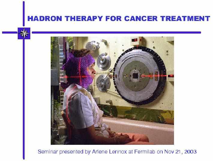
Figure 3: A very small group of people run the hadron therapy facility at Fermilab.

Users at Fermilab include summer students working on medical applicationsAmanda . To provide answers for visualization over such a broad range of applications is a difficult question.

Geant4 has done a very good job of making this question a little easier to answer by factoring the problem into visualization commands and drivers. The basic idea is that the visualization commands do not depend on the driver. Further it was hoped that once the code was built one could use any driver.The design was for the graphics systems to be complementary to each other. Because of the factorization this report will be about the different drivers.

II Documentation

This report is based on running on the latest version of Geant4 version v4_7_1. Some of my experience has been with earlier versions v4_6_2_p02, v4_7_0, and v4_7_0_p01. During this time the Geant4 graphics system has been stable. Version v4_7_1 was the first time I built an official Fermilab OpenGL version.

To learn about Visualization in Geant4 I have used chapter 8 (Visualization)of the Geant User’s Guide for Application DevelopersUsersGuide . The visualization chapter also covers visualization of detector geometry trees. These are easy to use (RegisterGraphicsSystem (new G4ASCIITree); Idle$>$ /vis/drawTree ! ATree), but are not relevant to our discussion on drivers. Visualization is also covered in a talk by Joseph Perl presented as part of a Geant4 tutorialPerl .

III Available Drivers

The list of drivers is given in Table 8.1 of the User’s Guide. The 11 possible choices are DAWNFILE, DAWN-Network, HepRepFile, OpenGL-Xlib, OpenGL-Motif, OpenGL-Win32, OpenInventor-X, OpenInventor-Win32, RayTracer, VRMLFILE, VRML-Network.

At Fermilab only Unix products are supported. At CERN there is support for running Geant4 under windows. Thus two choices are eliminated (OpenGL-Win32, OpenInventor-Win32). I have chosen not to investigate the network drivers. They are DAWN-Network, and VRML-Network. The OpenInventor drivers were developed at Fermilab by Jeff Kallenbach. At the present time no one is maintaining them. This eliminates OpenInventor-X from the list. Information about the RayTracer program can be found in the standard Geant4 source codeRayTracer . The documentation for RayTracer says that only a limited set of commands are supported. Further, the README says ”G4RayTracer can visualize absolutely all kinds of geometrical shapes which G4Navigator can deal with. Instead, it can NOT visualize hits nor trajectories generated by usual simulation” RayTracer it would seem would be valuable for finding problems in very complicated geometries. Because of it’s inability to deal with trajectories I have eliminated it. I have chosen to investigate OpenGL-Xlib, rather than OpenGL-Motif. In summary there are 4 general purpose drivers that will be investigated.

The remaining four drivers are: OpenGL-Xlib, VRMLFILE, HepRepFile and DAWNFILE. Thus I have run novice example3 with all of the four remaining drivers. Incidentally the talk by Joseph Perl is about three of the drivers (OpenGL, HepRepFile, DAWNFILE). The BTeV experiment (which included Rob Kutschke, Lynn Garren, Paul Lebrun, Julia Yarba, …) would have used VRMLFILE.

IV Tour of Visualization

IV.1 OpenGL

We start our tour with an OpenGL plot shown in Fig.4.

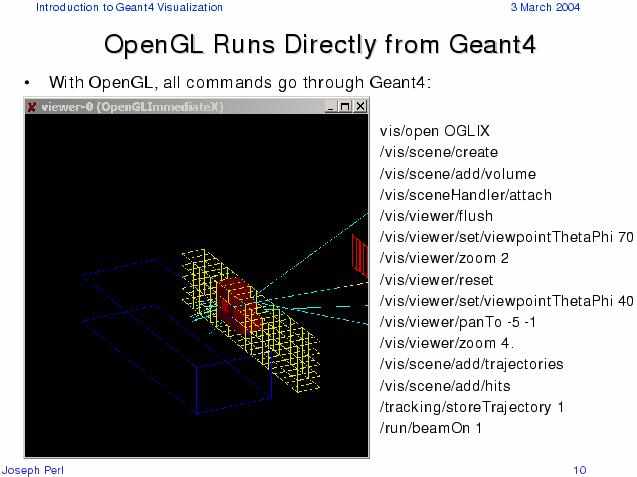
Figure 4: This is an OpenGL plot shown by Joseph Perl at the SLAC Mar. 2004 tutorial.

This is from a talk by Joseph Perl which was part of a Geant4 Tutorial held at SLAC in Mar.of 2004. The slide shows some typical Geant4 visualization commands. The first command /vis/open OGLIX opens the visualization driver. The title is very important and indicates that OpenGL runs directly from Geant4. All other drivers (HepRepFile, DAWNFILE and VRMLFILE) produce an intermediate file. It’s important to mention that the visualization code can be C++ source code or visualization commands. It’s very nice to be in the interactive mode and see the display change. Sometimes you may mistype a command and you learn that right away. It’s also important to realize that if you have many commands you can put them in a macro file (vis.mac). These commands can be executed at once by giving the command /control/execute vis.mac. Thus you can proceed efficiently in the interactive mode.

OpenGL plots have also been produced at Fermilab. The following plot shown in Fig. 5 created by V. Daniel Elvira is taken from our new Geant4 web pageNew_Web_Page .

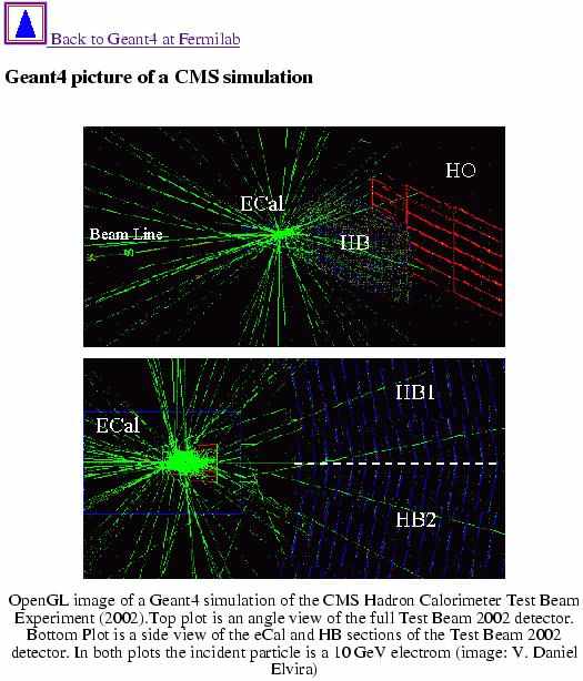
Figure 5: This is an OpenGL plot shown by Daniel Elvira at the Fermilab Oct. 2003 tutorial.

The web page has a section called pictures. Daniel’s plot is a simulation of an electron showering in the CMS EM calorimeter. Another OpenGL plot produced at Fermilab is shown in Fig. 6.

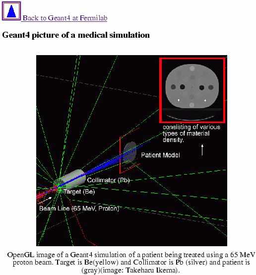
Figure 6: This is an OpenGL plot produced by Takeharu Ikema.

This plot was produced by a visitor Takeharu Ikema who worked on Medical Physics Applications.

IV.2 HepRep

We continue our tour by again looking at another plot from Joseph Perl’s talk (Fig.7).

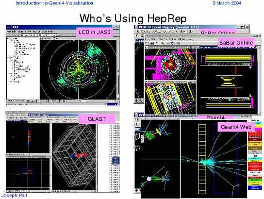
Figure 7: HepRep plots from a talk presented by Joseph Perl (Tutorial SLAC Mar. 2004).

This plot shows that HepRep is being used by many collaborations world wide. The plot in the upper left hand corner is made using JAS3 a general purpose, open-source data analysis tool. JAS is the abbreviation for JAVA Analysis Studio. The LCD indicates that this is a study for the Linear Collider Detector. Another important application for HepRep is the BeBar b-experiment at SLAC shown in the upper right corner. HepRep also serves the space community. GLAST is the Gamma Ray Large Array Telescope. The GLAST simulation is shown in the lower left hand corner. GLAST is scheduled to be launched in 2006GLAST . The lower right hand plot indicates that the Geant4 Web pages are maintained by using HepRep.

At Fermilab we (Andy Beretvas, V. Daniel Elvira and Panagiotis Spentzouris) have agreed to support HepRep. The reasons for our decision are that HepRep has menu’s to guide the user and is easy to install. Fig. 8 explains how using the WIRED client event display you can pick to show important features of the event (Particle ID, charge, momentum).

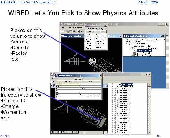
Figure 8: Picking important features of the event.
Also taken from Joseph Perl’s talk at SLAC Mar. 2004.

However, there are many reasons for this choice such as HepRep will work in a wider context. This is explained by Joseph Perl in Fig. 9.

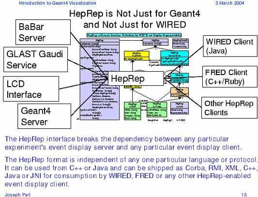
Figure 9: HepRep is not just for Geant4 is the title of this slide.
Also taken from Joseph Perl’s talk at SLAC Mar. 2004.

IV.3 DAWN

The next plot Fig. 10 shows a simulation of the ATLAS detector. Again the figure is taken from the talk by Joseph Perl. From the drawing the size of the detector is not clear. The detector is huge with a length of 45m and a height of 22m and contains more than million componentsAtlas_detector .

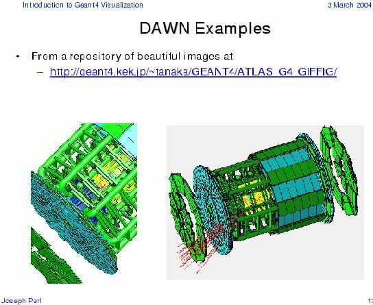
Figure 10: DAWN is used to display a simulation of the ATLAS detector.
Also taken from Joseph Perl’s talk at SLAC Mar. 2004.

I do not know of any Geant4 users at Fermilab who use DAWNFILE as a visualization driver.

IV.4 VRML

Here is a slide from the BTeV collaboration (Paul Lebrun) showing a pixel detector Fig. 11. This Geant4 slide is produced using the VRML driver.

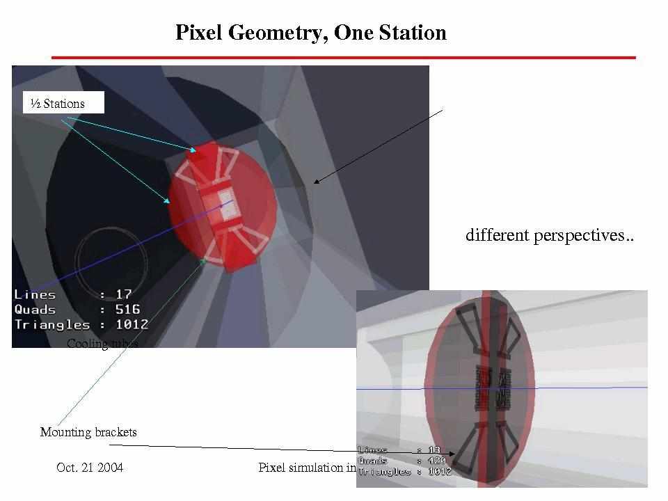
Figure 11: Geant4 using the VRML driver is used to produce a picture
of the proposed BTeV pixel detector.

The BTeV experiment was canceled in Feb. 2005BTeV . An experiment which is currently running (2005) is MiniBooNE. This is an experiment to test for neutrino mass by searching for neutrino oscillationsNeutrino_mass . Their GEANT4 simulation uses the VRML driver. A simulation of their beamline is shown in Fig. 12.

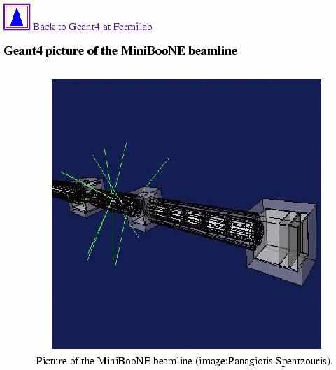
Figure 12: Geant4 using the VRML driver is used to produce a picture of the MiniBooNE beamline.

IV.5 OpenInventor

Although I have decided not to include the OpenInventor driver in our discussions, I was very impressed with the following figure (Fig. 13)

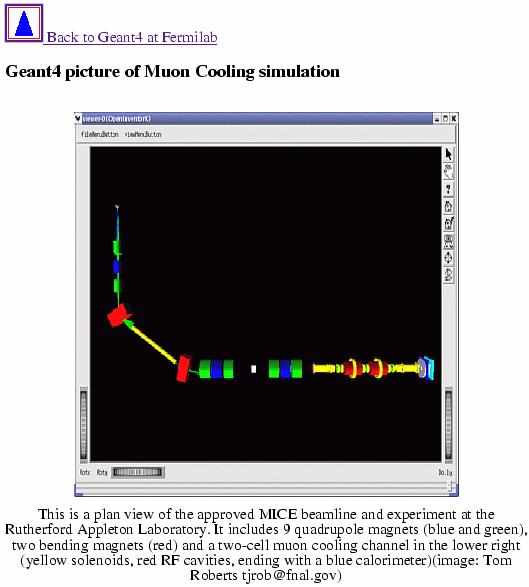
Figure 13: Simulation of MICE experiment using OpenInventor as the device driver (Tom Roberts).

provided by Tom Roberts. This figure is also available from the Fermilab Geant4 web page.

V Building OpenGL

In order to use some Visualization Drivers an external library must be used. There are five such libraries (OpenGL-Xlib, OpenGL-Motif, OpenInventor-X, Dawn-Network, and VRML-NetWork). Only one of then is among the 4 drivers we are investigating in this note (OpenGL-Xlib). The OpenGL version will be built for Fermilab users starting with v4_7_1. The build was done with the following command:
setenv G4VIS_BUILD_OPENGLX_DRIVER 1
To setup this version:
setup geant4 v4_7_1 -q GCC_3_4_3-OpenGL
You should get the correct flavor for your machine (either Scientific Linux, or Red Hat Linux). To correctly use this version you will need to indicate that you wish to use OpenGL and to obtain the libraries.
setenv G4VIS_USE_OPENGLX 1

setenv OGLHOME /usr/X11R6
setenv OGLFLAGS ”-I$OGLHOME/include”
setenv OGLLIBS ”-L/usr/X11R6/lib -lGL -lGLU”

VI Producing a plot from OpenGL

The first step is to produce an executable. In our example we use novice example N03. The instructions on doing this are documented on our web pageweb_instructions .

Next we produce a picture of the detector. Note this is the sampling calorimeter with layers of Pb and liquid Ar detection gaps. We run the job in interactive mode (./exampleN03). To clearly indicate the commands I am using I have put them in a macro file. We next execute the macro
Idle$>$ /control/execute vis_OpenGL0.mac
The macro file is shown in Fig. 14.

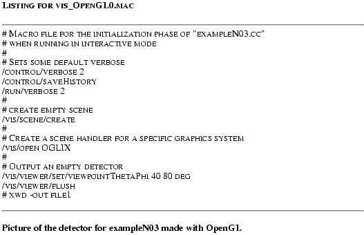
Figure 14: Example of a macro file used to produce an OpenGL plot. The plot shows the detector of novice example N03.

This produces a new window with the picture of the detector. A saved image of the picture is produced by opening another window. The window which has just been opened should be also in the area which contains the executable. In this window you type
xwd -out file.xwd
The name of the file is arbitrary. I will refer to this as an xwd file. This will produce a cursor, which you should place over the window which contains the picture. The program convert is then used to change the format of the file.
convert file0.xwd ex3_detector_OpenGL0.jpeg
I usually use a jpeg file for the web and an eps file for latex documents. The resulting plot is shown in Fig. 15.

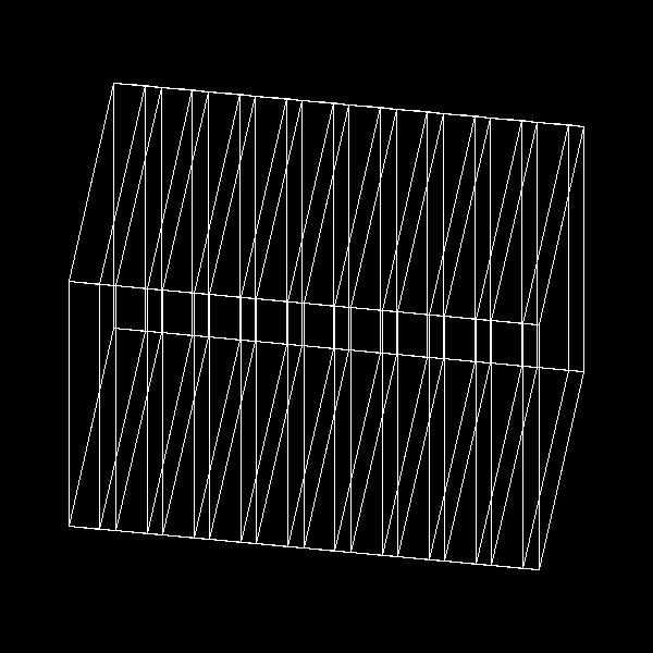
Figure 15: The calorimeter of example N03 produced using OpenGL.

The size of file0.xwd is 704 KBytes, and the size of the corresponding jpeg file is 51 KBytes. The size of the xwd file is determined by the number of pixels in the window. We now make a few changes in the macro and draw a plot for an interaction in the calorimeter. The few changes include specifying the incident particle and it’s energy. The macro file is given in Fig. 16.

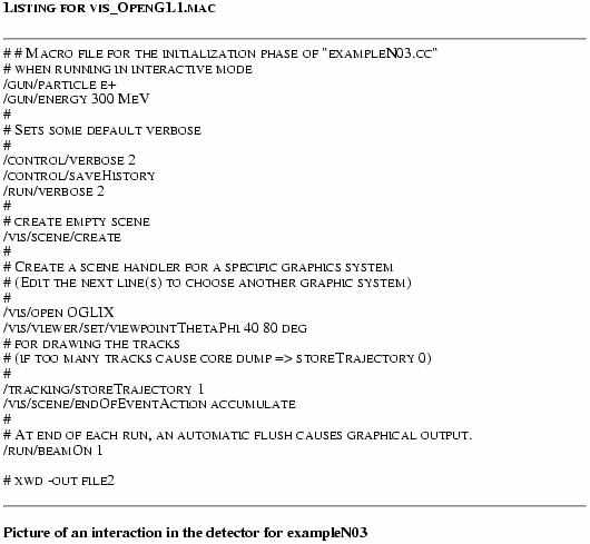
Figure 16: How to produce a plot using OpenGL for an interaction in the calorimeter.

The resulting plot is shown in Fig. 17.

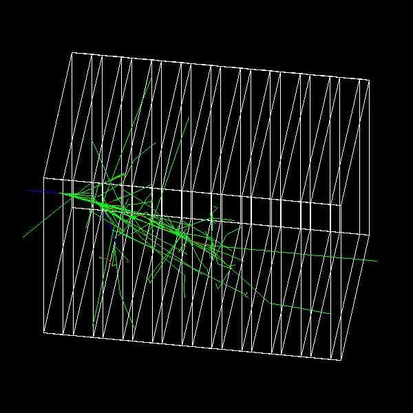
Figure 17: A positron of 300 MeV incident on the detector of example N03 (OpenGL).

On the screen the figure looks much better, because the green contrasts much better with the black (the black is not as intense as in the hardcopy). Geant4 uses the convention that negatively charged tracks are plotted in red, neutral in green and positive in blue. The size of the file is again the same (704 KBytes) as expected and the size of the corresponding jpeg file is 64 KBytes. We now run a third job accumulating all the hits for 10 events. The size of the file is again the same (704 KBytes) and the size of the jpeg file is 70 KBytes. The resulting very complicated plot is shown in Fig. 18.

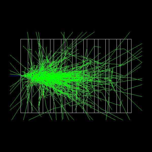
Figure 18: The superposition of 10 events in the detector of example N03.
Each event is initiated by a 300 MeV positron (OpenGL).

The size of the corresponding eps files is in all three cases 2144 KBytes. The information on the sizes of the OpenGL files is summarized in Table: 1.

Table 1: Sizes in KBytes for the OpenGL files

Name	xwd	jpeg	eps
Detector	704	51	2144
Detector + 1 event	704	64	2144
Detector + 10 events	704	70	2144

VII Producing many plots from OpenGL

The procedure described in the last section works well for a few plots, but real projects involve many plots. I am told by Don Holmgren that the Cryogenic Dark Matter people have developed a procedure using OpenGL and a virtual window to do this automatically.

VIII Using intermediate files

In principle you can use all drivers simultaneously. I have not yet tried this! First you must indicate which driver you are using. For the three drivers we will examine in detail the command is:
setenv G4VIS_USE_HepRepFile 1
setenv G4VIS_USE_DAWNFILE 1
setenv G4VIS_USE_VRMLFILE 1

The intermediate files have unique names in that the file is given an extension (.heprep, prim, wrl) for (HepRepFile, DAWNFILE, VRMLFILE) respectively.

VIII.1 Using HepRep

I run a single macro file that is almost equivalent to the three macro file used for OpenGL. The macro as expected uses /vis/open HepRepFile. This produces three data files (G4Data0.heprep, G4Data1.heprep and G4Data2.heprep). The size of these data files are 71, 1705, 16626 KBytes.

In order to proceed to look at these files the HepRep client file WIRED must be installed. The instruction for installing WIRED are given on a SLAC web pageSLAC_WIRED . I have installed wired in my own area on the FNALU Linux cluster and also on the cepa cluster ( andy/Wired/bin/wired). Additional information that maybe useful can be found in the Fermilab dictionary of Geant4 termsDictionary_WIRED . You will also want to learn about the HepRep Browser. To bring up the browser type:
 andy/Wired/bin/wired data_filedata_file
Information about the browser is available under Help -$>$ Quick Browser the first page is shown in Fig. 19.

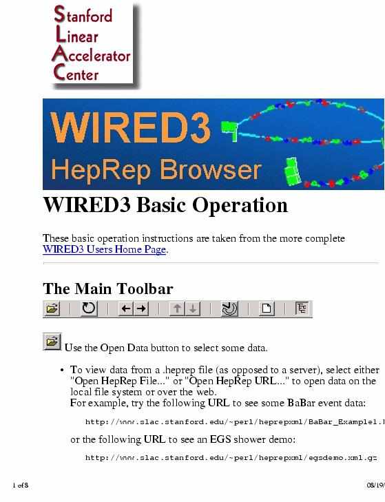
Figure 19: The first page of help for the HepRepBrowser..

The plots showing the detector, an interaction in the calorimeter and the superposition of 10 interactions are shown in Figures  20, 21 and  22.

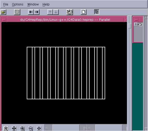
Figure 20: The calorimeter of example N03 produced using HepRep.

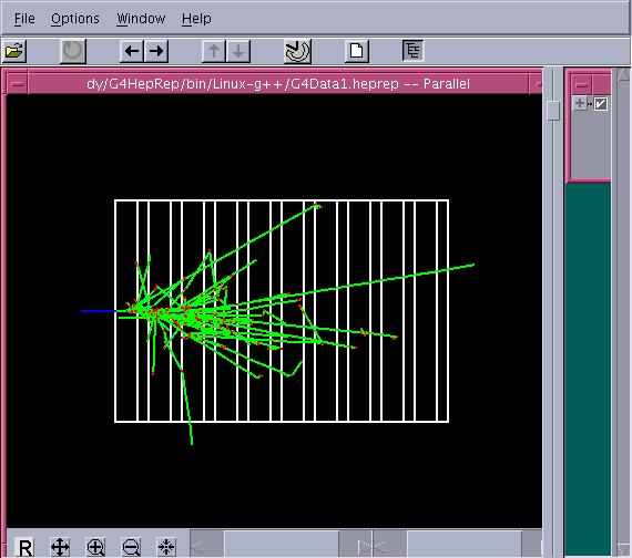
Figure 21: A positron of 300 MeV incident on the detector of example N03 (HepRep).

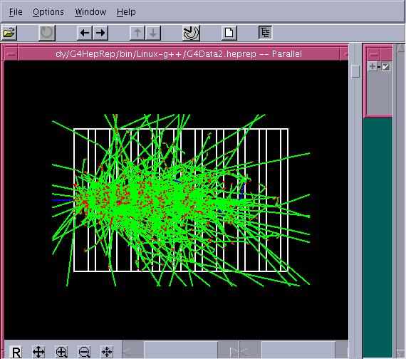
Figure 22: The superposition of 10 events in the detector of exampleN03.
Each event is initiated by a 300 MeV positron (HepRep).

On immediately notices that the command /vis/viewer/set/viewpointThetaPhi is not implemented, but one sees a standard view of the detector. I should point out that rotations around the axis perpendicular to the screen are allowed and more (see information in the Quick Browser under ”The Orientation Toolbar”).

The way to produce a plot is to go to ”File” and then ”Export Graphics”. I have recently encountered some difficulties with this and thus I have produced plots with xwd (see section on Producing a plot from OpenGL). HepRep keeps track of the files so that you can just click on the right arrow on the Main tool bar and it proceeds from the first file to the second file (G4Data0.heprep -$>$ G4Data1.heprep).

It takes a relatively long time (82 sec on my machine which is a 500 MHZ Pentium IIIMHZ ) to go from the second plot to the third This is clearly caused by the large size of the file and the fact that HepRep requires much information to be stored in it’s menus. As indicated earlier other information can be learned from the plots. For example that there are 469 tracks in the event see Fig. 21.

To set the material go to ”Options” and then ”Label Control” (see Fig 23).

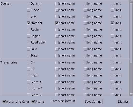
Figure 23: HepRep allows many options to be set including material.

The resulting plot is shown in Fig. 24.

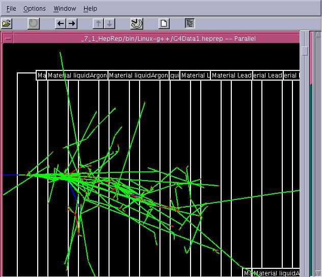
Figure 24: HepRep plot with the short version of the label for material.

One can see that the materials ”lead: and ”liquid Argon” appear on the plot, but to which region they refer is not so clear.

VIII.2 Using DAWN

The same macro is run as for HepRep, except for one command /vis/open DAWNFILE. This produces three data files (g4_00.prim, g4_01.prim and g4_02.prim). The size of the data files are 12, 235, and 2267 KBytes. Considerable smaller than the sizes of the HepRep files.

Again to proceed further the DAWN client must be installed. This is available form the web site of Satoshi Tanaka one of it’s developersTanaka . To install you will need to answer some questions, I think the default answer will work. On the fnalu cluster(flxi02,…) it is installed in  andy/dawn/dawn and on the cepa cluster in  andy/G4TEST/dawn_3_85e/PRIM_DATA/dawn.

The plots showing the detector, an interaction in the calorimeter and the superposition of 10 interactions are shown in Figures 25,

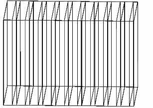
Figure 25: The calorimeter of example N03 produced using DAWN.

26

Figure 26: A positron of 300 MeV incident on the detector of example N03 (DAWN).

and  27.

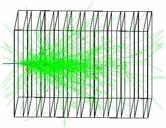
Figure 27: The superposition of 10 events in the detector of exampleN03.
Each event is initiated by a 300 MeV positron (DAWN).

One immediately notices that the command /vis/viewer/set/viewpointThetaPhi is now implemented.

The DAWN job runs immediately because of the smaller sized files and that no menu information is needed. What immediately means is 5 sec for the 10 event file. In running DAWN I have used the -d option this is for the direct mode. Further information is available dawn -h (see Fig. 28).

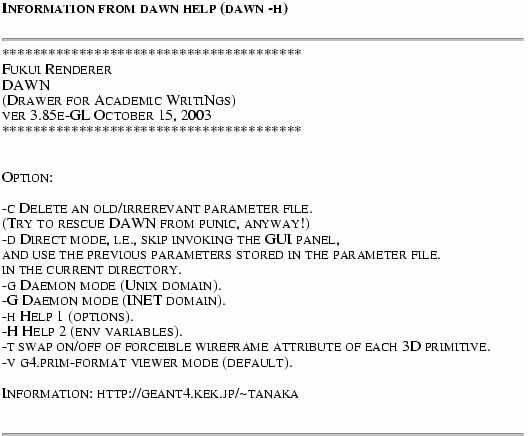
Figure 28: The help file for the DAWN display.

VIII.3 Using VRML

The same macro is run as for HepRep, except for one command /vis/open VRML1FILE. This produces three data files (g4_00.wrl, g4_01.wrl and g4_02.wrl). The size of the data files are 6, 141, and 1370 KBytes. Considerable smaller than the sizes of the HepRep files.

Again to proceed further the VRML client must be installed. Information about VRML can be found on the web3D_consortium . It is produced by ”Web3D Consortium- Open Standards for Real-Time 3D Communication Creators of the VRML (VRML1, VRML97, and now X3D, previously called VRML200x) open standards”. On cepa cluster the VRML client is in
/home/prj/bphys/releases/dev/vrmlview. On the fnalu cluster(flxi02,…) it is installed in  andy/vrmlview/vrmlview.

The plot showing the detector is in Fig. 29 and was produced by going to File and then ”Save snapshot”.

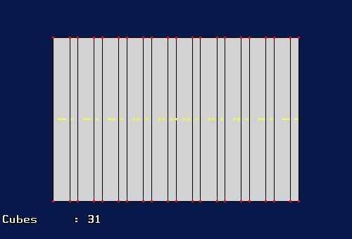
Figure 29: The calorimeter of example N03 produced using VRML.

We continue with our standard Fig. 30 of a positron entering the calorimeter.

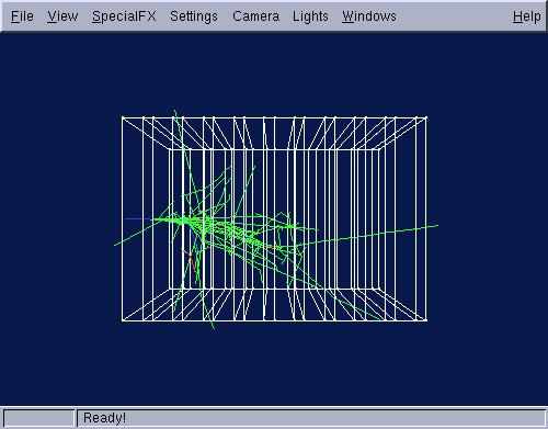
Figure 30: A positron of 300 MeV incident on the detector of example N03 (VRML).

This plot was produced by selecting under ”View” ”Wireframe” and ”Vertices”. However, it is easy to select options that do not produce a useful figure (see Fig.  31).

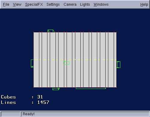
Figure 31: A positron of 300 MeV incident on the detector of example N03 (VRML). One can easily set the defaults such that the display is not useful.

Our standard final plot is shown in Fig. 32.

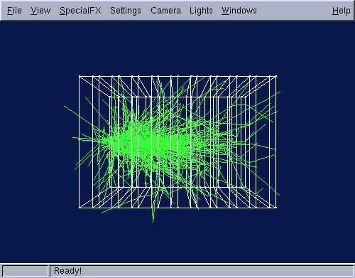
Figure 32: The superposition of 10 events in the detector of exampleN03.
Each event is initiated by a 300 MeV positron (VRML).

It takes 50 seconds for this plot to appear.

VIII.4 Summary of intermediate files

The size of the intermediate data files is summarized in Table  2.

Table 2: Sizes in KBytes for the intermediate files

Name	HepRep	DAWN	VRML
Detector	71	12	6
Detector + 1 event	1705	235	141
Detector + 10 events	16626	2267	1370

We see that if size is your major factor then VRML is the best choice and HepRep is the worst. In terms of menus to assist you HepRep is the best, the next best is VRML and last is DAWN. In terms of time DAWN is a clear winner 5 sec versus 50 sec for VRML and 82 sec for HepRep.In terms of quality plots DAWN is again the clear winner, followed by VRML and then HepRep.

IX Which driver to use?

The question of which driver to use was addressed by Joseph Perl. First he answers the list of what features are associated with each driver(see Fig 33).

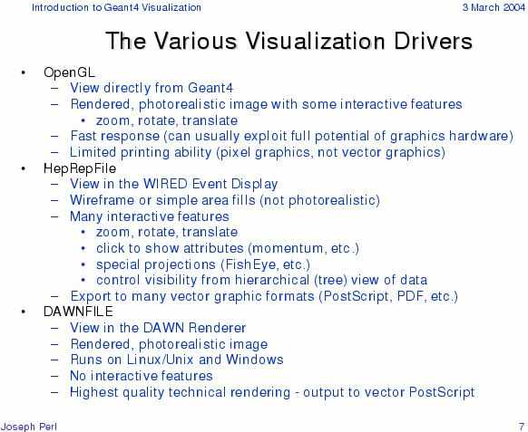
Figure 33: Features of the Visualization Drivers, OpenGL, HepRep and DAWN

To complete his slide I present the results for VRML in Fig. 34.

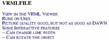
Figure 34: Features of the VRML Visualization Driver

Perl also indicates the circumstances in which you want to use the different drivers in Fig. 35.

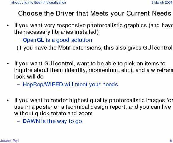
Figure 35: When to use a given driver from Joseph Perl SLAC Tutorial.

At Fermilab we have three different types of users, large experiments (CMS) medium experiments (MiniBooNE) and small experiments (neutron therapy).

The large experiments will want a structured environment. They may however, build it out of an environment that already has many of the tools like HepRep or they may want to proceed from a less structured environment like VRML. I strongly suspect that they will want their own graphics program. The Geant4 convention of only three colors (red, green, blue) for (neg, neutral, pos) is not what is needed for a modern high energy simulation program. One clearly needs different colors for electron and muons etc. The advice for the builders of a display for the Geant4 simulation program is to proceed exactly the way Geant4 has done and produce a program that is device independent! It would be even better if the builders of such a display program could get thir code incorporated into Geant4.

I suspect that medium sized experiments will want to go with HepRep because of the assistance provided by the menu’s.

Small experiments and starting students will want to use OpenGL because of it’s quick response. It also my favorite in the spirit of keeping things simple.

Clearly DAWN may be needed for publication quality work by large, medium and small experiments.

In Table3

Table 3: Graphics Summary

(1)= Best, (2) = Next Best
	1	2	3	4	5
Quality of plots	DAWN	OpenGL	VRML	HepRep
Menus	HepRep	VRML	DAWN	OpenGL
Time	OpenGL	DAWN	VRML	HepRep
Size of Files	OpenGL(jpeg)	VRML	OpenGL(eps)	DAWN	HepRep

I have attempted to summarized some of the important features for determining which device driver is right for you. The comparison of time and size of files is somewhat arbitrary when one compares the direct device driver and the those that use an intermediate file. I have left out the time required to produce the initial file for (HepRep, DAWN, VRML). Similarly I have not included the time to run OpenGL and produce the xwd file.

All four drivers are available on the central cluster, and the Geant4-team will try to assist you in obtaining the different driversgeant4-users . The issue of support has changed dramatically recently because of a suggestion by GP Yeh. It is now possible to run Geant4 on your own personal computer (Linux pc)geant4_pc . For pc user they will need to know how to obtain the client software. As this is all free software no serious problems are expected.

X Acknowledgments

I thank Randy Herber for his help with Latex.

References

- (1) I wish to thank V. Daniel Elvira for suggesting this topic.
-
(2)
CDF Internal note 0497 (June 1987)
A. Beretvas, F. Flintstone, J. Freeman, P.Hart, and GP Yeh -
(3)
F. Abe Phys. Rev. , 5550 (1994).
C. Avila Phys. Lett. , 419 (1999). -
(4)
CDF Internal note 4844 (Jan. 1999)
Comparison of the Total Cross Sections Measurements of CDF and E811
M. Albrow, A. Beretvas, L. Nodulman, P. Giromini -
(5)
Pier Oddone /5/16/05, A vision for Fermilab
http://vmsstreamer1.fnal.gov/VMS_Site_03/Lectures/EPP2010/050516Oddone/sld001.htm - (6) CMS Core Software Re-engineering Roadmap, the EDM design team Revision 1.34
-
(7)
OSCAR_3_9_6 is based on Geant v4_6_2_p02.
Unfortunately it still uses some of the old Geant3 code:
libG3Main.so and libG3Interface.so -
(8)
http://www-ed.fnal.gov/trc/sciencelines_online/Spring00/scientist.html
http://www.fnal.gov/culture/lecture.shtml
http://www-ppd.fnal.gov/EPPOffice-w/colloq/past_03_04.html -
(9)
I got Amanda Weinmann started on graphics with OpenGL.
Fermilab Today July 27, 2005
Fermilab Summer Students: Focus on Amanda Weinmann
http://www.fnal.gov/pub/today/archive_2005/today05-07-27.html -
(10)
CERN Documentation for User’s
http://wwwasd.web.cern.ch/wwwasd/geant4/G4UsersDocuments/UsersGuides/
ForApplicationDeveloper/html/Visualization/introduction.html -
(11)
Joseph Perl, SLAC Tutorial on Geant4.
http://geant4.slac.stanford.edu/g4cd/vol3/cd/Slides/agenda.html -
(12)
At Fermilab, setup Geant4 version