Complex energy approaches for calculating isobaric analogue states

Abstract

Two methods the complex energy shell model (CXSM) and the complex scaling (CS) approach were used for calculating isobaric analog resonances (IAR) in the Lane model. The IAR parameters calculated by the CXSM and the CS methods were checked against the parameters extracted from the direct numerical solution of the coupled channel Lane equations (CC). The agreement with the CC results was generally better than 1 keV for both methods and for each partial waves concerned. Similarities and differences of the CXSM and the CS methods are discussed. CXSM offers a direct way to study the configurations of the IAR wave function in contrast to the CS method.

I Introduction

The isobaric analogue resonances (IAR) have been discovered about four decades ago. They are the consequences of the approximate isospin symmetry. In the absence of isospin symmetry braking forces the analogue state would be degenerate with corresponding state of the parent nucleus. The Coulomb forces and isospin dependent interactions shift up the position of the analogue state and the analogue state may acquire a small width and may become a resonance.

The IAR has attracted interest in the latest development of the study of the light exotic nuclei. The unusual properties of neutron reach nuclei can provide insights into the nuclear structure far from the valley of stability. The extreme neutron to proton ratios may help to understand the nuclear matter at extreme conditions. However the experimental study of the neutron rich nuclei around the neutron drip line are difficult. Since the IAR has essentially the same structure as the parent state it was suggested that instead of the neutron reach exotic nuclei (${\rm{}^{11}Li}$, ${\rm{}^{14}Be}$, ${\rm{}^{7}He}$, ${\rm{}^{9}He}$) ter97 ; tak01 ; rog03 ; rog04 their less exotic analogue states should be studied (with inverse kinematics) to gain information about the properties of these exotic nuclei.

Recent developments in experimental facilities opened the possibility for identifying large number of exotic nuclei. To understand the structure of these nuclei new theoretical methods have been introduced for describing the dynamics of weakly bound or unbound nuclei from which nucleons can be emitted. Some of the new methods is e.g. the Shell Model in the complex energy plane (CXSM) rsm ; cxsm or the Gamow Shell Model mic ; mic03 ; mic07 ; mic07a ; rot06 use the Berggren basis b68 . In the Berggren basis bound and resonant states are treated on equal footed and scattering states taken along a contour $L$ of the complex energy sheet are included as it will be discussed later in detail. In the last few years this basis has been used successfully in a serious of works bet06 ; dus07 ; ve95 ; blo96 ; li96 . Since the extended use of this basis started not very long ago therefore we think that it is worthwhile to accumulate more experience concerning its accuracy and its dependence on their parameters.

Another well established method for calculating resonances is the complex scaling (CS) method. CS has a strict mathematical foundation given in Refs.ABC1 ; ABC2 ; ABC3 . The possible applications and the details of the CS method are reviewed in ho83 ; moi98 .

The IAR states phenomenologically can be described by the Lane equations lan or they can be studied by microscopically col98 . Coupled channel (CC) Lane equations offer a simple but not trivial (the simplest multichannel) example on which both the CXSM and the CS approaches can be checked.

Our aim in this work is to compare the parameters of the IAR calculated by different methods. We shall compare the characteristic features of the two methods working on the complex energy plane. The conclusion of such a methodical work can be useful later in analyzing experimental data in more realistic calculations.

The CS can be applied only for dilatation analytic potentials and interactions. However some of the widely used potentials in nuclear physics are not dilatation analytic or dilatation analytic only in a limited range of the rotation angle, i.e. below the critical value of the angle. Therefore we repeated our calculation with a slightly modified Coulomb potential which is dilatation analytic. This comparison is very useful to compare the accuracy of the CXSM and CS methods if they give the same results in cases when both methods can be applied.

In section II.1 we summarize the features of the Lane equations. In section II.2 we describe the approximate solution of the Lane equations using the CXSM, while in section II.3 we make a short description of the solution of the Lane equations using CS. In chapter III we give the numerical results of the calculations. In the first part of chapter III we compare the positions of the poles of the S-matrix calculated by the CXSM method with that extracted from the solution of the Lane equations. The results of the CS method are also presented here. The similarities and differences of the CXSM and CS methods are also discussed in that chapter. Finally in the last chapter we summarize the main conclusions of the paper.

II Resonance solution of the Lane equation

The Lane equations in the simplest case describe the quasi-elastic scattering of a proton and the IAR. We assume that the target nucleus has mass number $A=N+Z$ and charge number $Z$. The ground state of the target has isospin $T_{A}$ and isospin projection $T_{3}={\frac{N-Z}{2}}=T_{A}$. The target is bombarded by a beam of protons.

II.1 Lane equation

The Hamiltonian of the target plus nucleon system $H$ can be divided to a part describing the internal motion of the target $H(\xi)$ and their relative motion $H_{rel}$

$$H=H(\xi)+H_{rel}~{}.$$ (1)

The internal state of the ground state of the target is denoted by $|A\rangle$ and this state is the solution of the equation $H(\xi)|A\rangle=\epsilon_{A}|A\rangle$. The analog nucleus is denoted by $\tilde{A}$ it has the same isospin $T_{A}$ and isospin projection $T_{A}-1$. It is an excited state of the isobaric nucleus with $Z+1$ protons and $N-1$ neutrons. If we neglect the mass difference between the neutron and proton and denote the additional Coulomb energy of the analogue nucleus by $\Delta_{c}$ then the eigenvalue of the internal motion of the analogue state is simply $\epsilon_{A}+\Delta_{c}$ and we have $H(\xi)|\tilde{A}\rangle=(\epsilon_{A}+\Delta_{c})|\tilde{A}\rangle$. Let $|pA\rangle$ and $|n\tilde{A}\rangle$ be the states formed by adding a proton and neutron to $|A\rangle$ and $|\tilde{A}\rangle$, respectively. The total wave function of the system may be written in the form

$$\Psi=|A\rangle\phi_{p}({\bf r})+|\tilde{A}\rangle\phi_{n}({\bf r}),$$ (2)

where $\phi_{p}({\bf r})$ and $\phi_{n}({\bf r})$ describe the relative motion. The relative motion part of the total Hamiltonian can be cast into the form

$$H_{rel}=K+V_{0}({\bf r})+{\bf\hat{t}}\cdot{\bf\hat{T}}V_{1}({\bf r})+({\frac{1}{2}}-t_{3})V_{C}(r)~{},$$ (3)

where $K$ is the kinetic energy operator of the relative motion, $V_{0}$ comes from the interactions independent form the isospin, $V_{C}$ is the nuclear Coulomb potential and ${\bf\hat{t}}\cdot{\bf\hat{T}}V_{1}({\bf r})$ is the symmetry term due to the isospin dependent strong interactions. The vector operators $\bf\hat{t}$ and $\bf\hat{T}$ are the isospin operators of the nucleon and that of the target. Substituting the ansatz (2) into the Schrödinger equation $H\Psi={\cal E}\Psi$ and taking into account the form (3) of the relative Hamiltonian we get the Lane equations lan :

$$\left[K+V_{0}-{{\frac{1}{2}}}T_{A}V_{1}+V_{C}-{\cal E}_{p}\right]\phi_{p}+\sqrt{{\frac{1}{2}}T_{A}}V_{1}\phi_{n}=0$$

$$\left[K+V_{0}+{{\frac{1}{2}}}(T_{A}-1)V_{1}-({\cal E}_{p}-\Delta_{c})\right]\phi_{n}+\sqrt{{\frac{1}{2}}T_{A}}V_{1}\phi_{p}=0,$$ (4)

where ${\cal E}_{p}={\cal E}-\epsilon_{A}$ is the center-of-mass energy of the relative motion of the proton plus target system and the relative energy for the neutron plus analogue nucleus is ${\cal E}_{p}-\Delta_{c}$. If we assume that the interactions are spherical symmetric then the relative motion can be divided into partial waves and there are no coupling between different partial waves characterized by orbital $l$ and total angular momentum $j$ quantum numbers. The numerical solution of the Lane equation has been carried out by using fourth order Runge-Kutta method. At each real ${\cal E}_{p}$ values we calculated two linearly independent solutions of the coupled equations. The physical solution with components $\phi_{p}$ and $\phi_{n}$ being regular at $r=0$ was combined from these independent solutions. These components $\phi_{p}$ and $\phi_{n}$ were matched to the scattering (or outgoing wave) solutions of the corresponding channels at a distance where the nuclear potentials are cut to zero. This is a standard method described e.g. in Ref. toboc .

II.2 CXSM a solution using Berggren basis

In this section we calculate the complex energy eigenvalues of the IAR by diagonalizing the Hamiltonian (1) in combined Berggren bases b68 of the target plus proton and analog plus neutron systems. First we describe the Berggren basis for the protons. We consider an auxiliary problem, a radial Schrödinger equation with the diagonal potential of the first equation of the Lane equation (II.1)

$$\left[K_{l}+V_{0}-{{\frac{1}{2}}}T_{A}V_{1}+V_{C}-E_{n}^{(p)}\right]u^{(p)}_{n}(r)=0,$$ (5)

where

$$K_{l}=-{\frac{\hbar^{2}}{2\mu}}\left[{\frac{d^{2}}{dr^{2}}}-{\frac{l(l+1)}{r^{2}}}\right].$$ (6)

The discrete bound and resonance solution with energy $E_{n}^{(p)}$ are denoted by $u^{(p)}_{n}(r)$ and the scattering solutions by $u^{(p)}(r,E)$. Sometimes when it is obvious we will use the wave number $k$ instead of the energy $E$ and the scattering states along the contour in the lower half of the second energy sheet will be denoted by $u^{(p)}(r,k)$.

The main advantage of the Berggren basis is that the single-particle basis set consists not only of bound states but also of poles of the single-particle Green function on the complex energy (wave number) planes and a continuum of scattering states taken along a complex contour $L$. A typical contour of the complex wave number plane is shown in Fig. 1. The $L^{+}$ part of the contour goes from the origin to infinity in the lower half of the second energy sheet, while the $L^{-}$ part of the contour makes exactly the same tour on the first energy sheet. It was observed in Refs. Hag06 ; Myo98 that the contour $L^{+}$ need not return to the real axis at infinity. The shape of the chosen complex contour $L=L^{+}+L^{-}$ regulates which of the poles should be included into the Berggren basis forming the completeness relation of Berggren:

$$\delta(r-r^{\prime})=\sum_{n=b,d}{u^{(p)}_{n}(r)}u^{(p)}_{n}(r^{\prime})+2\int_{L^{+}}dk{u^{(p)}(r,k)}u^{(p)}(r^{\prime},k)~{}.$$ (7)

In this relation (and later) the notation $n=b,d$ means that the sum over $n$ runs through all bound states plus the decaying resonances lying between the real energy axis and the integration contour $L^{+}$ of Fig. 1. The integral in Eq. (7) is over the scattering states along $L^{+}$ (factor $2$ is due to the symmetry of $L$). The poles denoted by $d$ in the basis generally correspond to decaying resonances lying on the fourth quadrant of the complex $k$-plane.

The completeness relation in Eq. (7) was introduced for charge less particles in Ref. b68 and it has been shown later in Ref. Michel that it is valid even for charged particles. Berggren completeness can be generalized by using a contour of different shape in which antibound states i05 lying on the negative part of the imaginary $k$-axis are included in the sum in Eq. (7). Since the inclusion of antibound states is not optimal as far as the number of basis states is concerned Naza we are not using antibound basis states in this work.

Figure 1: Positions of the bound ($b_{1}$, $b_{2}$) and decaying resonant ($d_{1}$, $d_{2}$) poles of $S(k)$ on the complex $k$-plane and a possible choice of the complex contour $L$ .

Berggren introduced a generalized scalar product between functions defining a special complex metric of the Berggren space b68 . In the generalized scalar product in the left (bra) position of the scalar product the mirror partner state (denoted by tilde over the state) is used. This state corresponds to the reflection to the imaginary $k$-axis. Due to this reflection in this scalar product in the integration the radial wave functions appears instead of the complex conjugate of the radial function. (This causes no difference for bound (and anti-bound) states lying on the imaginary axis.) This is the only modification in the scalar product since the spin-angular degrees of freedom remains unchanged. If the radial integral to be calculated has no definite value then a regularization procedure has to be applied. Zel’dovich zel and also Romo rom suggested regularization methods but we use the complex rotation of the radial distance $r$ beyond the range of nuclear forces gyar .

The upper half of the complex $k$-plane maps to the physical (or first) Riemann-sheet of the complex energy $E\sim k^{2}$. The pole wave functions of this sheet are square integrable functions belonging to bound states. While the lower half of the complex $k$-plane maps to the unphysical (or second) Riemann-sheet of the energy $E$. The pole wave functions of the second sheet are not square integrable functions and they belong to decaying/capturing resonances lying on the lower/upper part of that energy sheet or antibound states lying on the negative real energy axis. The calculation of integrals in which these radial wave functions appear might need the use of regularization procedure.

Since the number of basis states has to be finite the complex continuum has to be discretized. It is preferable to use as discretization points $E_{i}^{(p)}$ the abscissas of a Gaussian quadrature procedure and the corresponding weights of that procedure are denoted by $h_{i}$. By discretizing the integral in Eq. (7) one obtains an approximate completeness relation for the finite number of basis states:

$$\delta(r-r^{\prime})\approx\sum_{n=b,d,c}^{M}{w^{(p)}_{n}(r,E^{(p)}_{n})}w^{(p)}_{n}(r^{\prime},E^{(p)}_{n}),$$ (8)

where $c$ labels the discretized contour $L^{+}$ states. If $E^{(p)}_{n}$ corresponds to scattering energy from the contour $L^{+}$ then the scattering state of the discretized continuum is denoted by $w^{(p)}_{n}(r,E^{(p)}_{n})=\sqrt{h_{n}}u^{p}_{n}(r,E^{(p)}_{n})$ and if $E^{(p)}_{n}$ corresponds to a normalized pole state then $w^{(p)}_{n}(r,E^{(p)}_{n})=u^{(p)}_{n}(r)$. The set of Berggren vectors form a bi-orthonormal basis in the truncated space

$$<\tilde{w}^{(p)}_{n}|w^{(p)}_{m}>=\delta_{n,m}~{}.$$ (9)

The Berggren basis for neutrons is defined similarly but the auxiliary problem uses the diagonal part of the second equation of (II.1)

$$\left[K_{l}+V_{0}+{{\frac{1}{2}}}(T_{A}-1)V_{1}-E^{(n)}_{n}\right]u^{(n)}_{n}({r})=0.$$ (10)

Having fixed the Berggren basis for neutrons and protons we take the ansatz (2) but the relative motion functions are expanded on the corresponding Berggren basis

$$\phi_{p}({\bf r})=\left[\sum_{i=1}^{M_{p}}C^{(p)}_{i}w^{(p)}_{i}({r},E^{(p)}_{i})\right]{\cal Y}_{ljm}$$ (11)

and

$$\phi_{n}({\bf r})=\left[\sum_{i=1}^{M_{n}}C^{(n)}_{i}w^{(n)}_{i}({r},E^{(n)}_{i})\right]{\cal Y}_{ljm}~{},$$ (12)

where ${\cal Y}_{ljm}$ denotes the spin-angular part of the wave function. Using Eq. (II.1) we get the following set of linear equations for the unknown complex expansion coefficients $C^{(p)}_{i}$ and $C^{(n)}_{i}$

$$(E^{(p)}_{k}-{\cal E}_{p})C^{(p)}_{k}+\sum_{m=1}^{M_{n}}\langle\tilde{w}^{(p)}_{k}|\delta v|w^{(n)}_{m}\rangle C^{(n)}_{m}=0$$

$$k=1,\ldots,M_{p}$$ (13)

and

$$(E^{(n)}_{k}-({\cal E}_{p}-\Delta_{c}))C^{(n)}_{k}+\sum_{m=1}^{M_{p}}\langle\tilde{w}^{(n)}_{k}|\delta v|w^{(p)}_{m}\rangle C^{(p)}_{m}=0$$

$$k=1,\ldots,M_{n},$$ (14)

where the coupling potential is $\delta v=\sqrt{\frac{T_{A}}{2}}V_{1}$. The above two equations can be combined into one matrix eigenvalue equation with dimension $M_{p}+M_{n}$. By diagonalizing the matrix of the Hamiltonian we get $M_{p}+M_{n}$ complex eigenvalues ${\cal E}^{\nu}_{p}$ $\nu=1,\ldots M_{p}+M_{n}$. One of the complex eigenvalues ${\cal E}^{\nu}_{p}$ is identified by the energy of the IAR. The identification in general is easy because most of the other unbound states correspond to discretized contour states and they are lying far from the position of the IAR at ${\cal E}_{IAR}=E_{r}-i{\frac{\Gamma}{2}}$ and in the wave function of the IAR the dominant component is a bound neutron state.

II.3 Complex scaled Lane equation

The poles of the Green-operator on the complex energy plane can be determined with the help of the complex scaling. The CS mathematically well founded ABC1 ; ABC2 ; ABC3 and has many applications in atomic, molecular and nuclear physics. We demonstrate the effect of the CS on an example of a single-particle Hamiltonian $\hat{h}$. The real angle $\theta$ of the CS rotates the coordinates of the particle to complex, i.e. $\bf r$ is simply replaced by $\exp(i\theta){\bf r}$. More precisely the effect of the CS can be given with the help of an operator ${\hat{U}}(\theta)$. It acts on an arbitrary function $g({\bf r})$ as

$${\hat{U}}(\theta)g({\bf r})=\exp(i{\frac{3}{2}}\theta)g({\bf r}e^{i\theta})~{}.$$ (15)

The complex scaled Hamiltonian is the following

$${\hat{h}}_{\theta}={\hat{U}}_{\theta}{\hat{h}}{\hat{U}}_{\theta}^{-1}~{}.$$ (16)

The kinetic energy $\hat{K}=-\frac{\hbar^{2}}{2\mu}\Delta_{\bf r}$ transforms due to the complex scaling to

$${\hat{U}}_{\theta}{\hat{K}}{\hat{U}}_{\theta}^{-1}=\exp(-i2\theta)(-\frac{\hbar^{2}}{2\mu}\Delta_{\bf r})~{},$$ (17)

and a local potential ${\hat{V}}(\bf r)$ transforms to the form:

$$\hat{V}^{\theta}({\bf r})={\hat{U}}_{\theta}{\hat{V}}({\bf r}){\hat{U}}_{\theta}^{-1}={\hat{V}}({\bf r}\exp(i\theta))~{}.$$ (18)

Assume that $\chi_{\nu}(\bf r)$ is a bound or resonance eigenfunction of the the Hamiltonian $\hat{h}$ and the corresponding eigenvalue is $E_{\nu}$ then the function $\chi_{\nu}^{\theta}({\bf r})=\exp(i{\frac{3}{2}}\theta)\chi_{\nu}({\bf r}e^{i\theta})$ will be the eigenfunction of the complex scaled Hamiltonian ${\hat{h}}_{\theta}$ with the same eigenvalue $E_{\nu}$. The advantage of the CS is that the function $\chi_{\nu}^{\theta}({\bf r})$ is square integrable even if the original state was a resonance wave function. The square integrability of $\chi_{\nu}^{\theta}({\bf r})$ allows that it can be approximated well with finite expansion using only square integrable basis functions.

The Lane equation can be considered as an eigenvalue problem of a two by two matrix Hamiltonian

$${\cal H}=\left(\begin{array}[]{cc}K+V_{0}-{\frac{T_{A}}{2}}V_{1}+V_{C}&\ \ \sqrt{\frac{T_{A}}{2}}V_{1}\\ \sqrt{\frac{T_{A}}{2}}V_{1}&\ \ K+V_{0}+{\frac{T_{A}-1}{2}}V_{1}+\Delta_{c}\end{array}\right)~{}.$$ (19)

The Lane-equation (II.1) can be cast into the form

$${\cal H}\left(\begin{array}[]{c}\phi_{p}({\bf r})\\ \phi_{n}({\bf r})\end{array}\right)={\cal E}_{p}\left(\begin{array}[]{c}\phi_{p}({\bf r})\\ \phi_{n}({\bf r})\end{array}\right).$$ (20)

The generalization of the operator $\hat{U}_{\theta}$ is straightforward

$${\cal U}_{\theta}=\left(\begin{array}[]{cc}U_{\theta}&0\\ 0&U_{\theta}\end{array}\right)$$ (21)

and the complex scaled matrix Hamiltonian is ${\cal H}_{\theta}={\hat{\cal U}}_{\theta}{\cal H}{\hat{\cal U}}_{\theta}^{-1}$. The eigenvalue problem of this operator

$${\cal H}_{\theta}\left(\begin{array}[]{c}\phi^{\theta}_{p}({\bf r})\\ \phi^{\theta}_{n}({\bf r})\end{array}\right)={\cal E}^{\theta}_{p}\left(\begin{array}[]{c}\phi^{\theta}_{p}({\bf r})\\ \phi^{\theta}_{n}({\bf r})\end{array}\right)$$ (22)

in components gives the following set of equations

$$\left[H_{p}^{\theta}-{\cal E}^{\theta}_{p}\right]\phi^{\theta}_{p}+\sqrt{\frac{1}{2}T_{A}}V_{1}^{\theta}\phi^{\theta}_{n}=0$$

$$\left[H^{\theta}_{n}-{\cal E}^{\theta}_{p}\right]\phi^{\theta}_{n}+\sqrt{\frac{1}{2}T_{A}}V_{1}^{\theta}\phi^{\theta}_{p}=0~{},$$ (23)

where $H^{\theta}_{p}=\exp(-i2\theta)K+V^{\theta}_{0}-\frac{1}{2}T_{A}V^{\theta}_{1}+V^{\theta}_{C}$ and $H^{\theta}_{n}=\exp(-i2\theta)K+V^{\theta}_{0}+\frac{1}{2}(T_{A}-1)V^{\theta}_{1}+\Delta_{c}$. We will refer to (II.3) as complex scaled Lane-equation. Since the functions $\phi^{\theta}_{p}({\bf r})$ and $\phi^{\theta}_{n}({\bf r})$ are square integrable we can make the approximation

$$\phi^{\theta}_{p}({\bf r})=\left[\sum_{i=1}^{M_{p}}C^{(p,\theta)}_{i}\psi_{i}^{(p)}({r})\right]{\cal Y}_{ljm}$$ (24)

and

$$\phi^{\theta}_{n}({\bf r})=\left[\sum_{i=1}^{M_{n}}C^{(n,\theta)}_{i}\psi_{i}^{(n)}({r})\right]{\cal Y}_{ljm},$$ (25)

where $\psi_{i}^{(n)}({r})$ and $\psi_{i}^{(p)}({r})$ are arbitrary square integrable basis functions. Substituting these forms into the (II.3) we get a matrix eigenvalue equation. In details we have

$$\sum_{m=1}^{M_{p}}\langle\tilde{\psi}_{k}^{(p)}|H^{\theta}_{p}|\psi_{m}^{(p)}\rangle C^{(p,\theta)}_{m}+\sum_{m=1}^{M_{n}}\langle\tilde{\psi}_{k}^{(p)}|\delta v^{\theta}|\psi_{m}^{(n)}\rangle C^{(n,\theta)}_{m}$$

$$={\cal E}_{p}\sum_{m=1}^{M_{p}}\langle\tilde{\psi}_{k}^{(p)}|\psi_{m}^{(p)}\rangle C^{(p,\theta)}_{m}\ \ \ k=1,\ldots,M_{p},$$ (26)

and

$$\sum_{m=1}^{M_{n}}\langle\tilde{\psi}_{k}^{(n)}|H^{\theta}_{n}|\psi_{m}^{(n)}\rangle C^{(n,\theta)}_{m}+\sum_{m=1}^{M_{p}}\langle\tilde{\psi}_{k}^{(n)}|\delta v^{\theta}|\psi_{m}^{(p)}\rangle C^{(p,\theta)}_{m}$$

$$={\cal E}_{p}\sum_{m=1}^{M_{n}}\langle\tilde{\psi}_{k}^{(n)}|\psi_{m}^{(n)}\rangle C^{(n,\theta)}_{m}\ \ \ k=1,\ldots,M_{n}.$$ (27)

The solution of these equations provide us $M_{p}+M_{n}$ number of complex eigenvalues. The majority of these eigenvalues correspond to the discretization of the rotated down continuous spectrum. The bound and resonance poles can be clearly identified and the accurate value can be determined using the so called $\theta$ trajectory technique.

III Numerical results

We applied the methods described in section II.2 and II.3 for the description of the IAR-es in the ${\rm{}^{209}Bi}$ nucleus with large neutron excess. We studied several analogue resonances in the ${\rm p+^{208}Pb}$ system. For illustrative purposes we selected an IAR which in our simple model is the analog of the ground state of ${\rm{}^{209}Pb}$, i.e. a $g_{9/2}$ single particle state. The effect of the double magic core is described by a phenomenological potential. We used Woods-Saxon (WS) forms for both the diagonal and the coupling potentials in (II.1). The WS forms cut to zero at a finite distance: $R_{max}=20$ fm

$$V^{WS}_{tr}(r)=\left\{\begin{array}[]{rl}V^{WS}(r)&\textrm{ if }r~{}<~{}R_{max}\\ 0&\textrm{ if }r~{}\geq~{}R_{max}~{}.\end{array}\right.$$ (28)

The spin-orbit part of the potential has the usual derivative form:

$$V_{so}^{WS}(r)=-\frac{V_{so}}{ra}~{}2(\vec{l}\cdot\vec{s})\frac{e^{\frac{r-R}{a}}}{(1+e^{\frac{r-R}{a}})^{2}}~{}.$$ (29)

It is also cut to zero at $R_{max}$. The numerical values of the potential parameters were taken from an early work gyave . For the sake of simplicity the radii and the diffuseness were taken the same values for protons and neutrons and for the common spin-orbit term: $r_{0}=1.19$ fm and $a=0.75$ fm, $V_{so}=11.6$ MeV. For Coulomb potential we assumed that the charge $Ze$ of the target is homogeneously distributed inside a sphere with radius $R_{c}=r_{c}A^{1/3}$ with sharp edge

$$V_{C}(r)=Ze^{2}\left\{\begin{array}[]{rl}\frac{1}{2R_{c}}[3-(\frac{r}{R_{c}})^{2}]&\textrm{ if }r\leq R_{c}\\ 1/r&\textrm{ if }r>R_{c}~{}.\end{array}\right.$$ (30)

The depth of the nucleon potential was $56.4$ MeV and the strength of the symmetry potential was $0.5$ MeV. Therefore the diagonal WS potential felt by the proton was $61.9$ MeV and by the neutron $51.15$ MeV according to the Lane equations in Eq. (II.1). The Coulomb radius was identical with the one of the nuclear potential. The Coulomb energy difference was also the same as in Ref. gyave $\Delta_{c}=18.9$ MeV.

State	neutron	proton(Eq. (30))	proton(Eq. (32))
$1g_{9/2}$	$(-22.878,0.0000)$	$(-11.894,0.0000)$	$(-13.975,0.0000)$
$2g_{9/2}$	$(-4.060,0.0000)$	$(7.674,-6.210^{-4})$	$(6.070,-2.010^{-5})$

Table 1: Energies of the discrete $g_{9/2}$ single-particle basis states for neutrons and for protons corresponding to the Woods-Saxon potential described in the text. The Coulomb potential for protons is either the usual one in Eq. (30) or the dilatation analytic one in Eq. (32). Energies are in MeV.

In the CXSM the elements of the single particle bases are calculated in the diagonal potentials appearing in the corresponding channels of the Lane equations. The single particle energies for the $g_{9/2}$ neutron and proton orbits are summarized in Table 1. The vertexes of three different proton and neutron $L$ contours for the $g_{9/2}$ case are shown in Table 2. The numbers of the discretization points $N_{i}$ of the segment $[V_{i},V_{i+1}]$ are shown between the vertex points. To calculate IAR-es we could use neutron contours taken along the real axis. For other partial waves we used large variety of contours.

Channel	proton			neutron
Contour	$LP1$	$LP2$	$LP3$	$LN1$	$LN2$	$LN3$
$V_{0}$	(0,0)	(0,0)	(0,0)	(5,-0.4)	(5,-0.35)	(3,0)
$N_{0}$	0	0	4	0	0	10
$V_{1}$	(5,-0.4)	(5,-0.35)	(5,-0.4)	(30,-0.4)	(30,-2.098)	(3,-10)
$N_{1}$	78	34	22	0	0	4
$V_{2}$	(30,-0.4)	(30,-2.098)	(30,0)	(30,0)	(100,-6.993)	(10,-10)
$N_{2}$	2	4	2	0	0	6
$V_{3}$	(30,0)	(100,-6.993)	(100,0)	(100,0)		(10,0)
$N_{3}$	0		4	0	0	4
$V_{4}$	(100,0)		(200,0)	(200,0)		(30,0)
$N_{4}$	0			0	0	0
$V_{5}$	(200,0)					(100,0)

Table 2: Integration contours for $g_{9/2}$ protons and neutrons given by vertexes $V_{i}$ (in MeV) and the number of Gaussian points $N_{i}$. The $N_{i}$ values are the ones necessary to reach the $1$ keV accuracy for the IAR or for the broad resonance at ${\cal E}_{p}=(23.996,-6.147)$ MeV. Contours LP3 and LN3 were used for the broad resonance.

In the CC method we solved the coupled Lane equations for a fine equidistant mesh of the bombarding proton energy ${\cal E}_{p}={\cal E}_{0},{\cal E}_{0}+d{\cal E},...,{\cal E}_{max}$ in the center of mass system and calculated the scattering matrix elements for each energy values: $S({\cal E}_{p})$.

In order to determine the parameters of the IAR we fitted the tabulated values of the $S({\cal E}_{i})$ by the following form:

$$S({\cal E}_{p})=e^{2i\delta_{p}({\cal E}_{p})}(1-i\frac{\Gamma_{p}}{{\cal E}_{p}-\cal{E}_{IAR}})~{},$$ (31)

where $\cal{E}_{IAR}$ denotes the complex energy of the IAR, i.e. ${\cal E}_{IAR}=E_{r}-i{\frac{\Gamma}{2}}$, $\Gamma$ is the full width and $\Gamma_{p}$ is the proton partial width of the IAR. Below the threshold of the ${}^{208}Pb(p,{\bar{n}})^{208}Bi$ reaction the total width is equal to the the partial width: $\Gamma=\Gamma_{p}$ in our model. Equation (31) represents a one pole approximation to the S-matrix in the proton channel.

For the background phase shift in the entrance channel $\delta_{p}({\cal E}_{p})$ we take a linear energy dependence in order to better reproduce the non-resonant background. Naturally all these quantities refer to definite ${\rm l,j}$ partial waves. The best fit parameter values are listed in the $E_{r}(CC)$ and $\Gamma(CC)$ columns in Table 3. The one pole formula of (31) gave excellent fit to the tabulated values of $S({\cal E}_{i})$ in all cases in Table 3.

$l~{}j$	$E_{r}(CXSM)$	$E_{r}(CC)$	$\Gamma(CXSM)$	$\Gamma(CC)$
$g_{9/2}$	14.954	14.954	0.046	0.047
$i_{11/2}$	15.526	15.526	0.003	0.003
$d_{5/2}$	16.445	16.444	0.141	0.140
$s_{1/2}$	16.918	16.917	0.156	0.156
$g_{7/2}$	17.367	17.367	0.086	0.084
$d_{3/2}$	17.441	17.440	0.144	0.145
$j_{15/2}$	18.774	18.774	0.006	0.006

Table 3: Comparison of the IAR parameters calculated by using the CC and CXSM methods for different partial waves with Coulomb potential Eq. (30). Energies are in MeV units.

The numerical values of ${\cal E}_{IAR}$ are shown as $E_{r}(CXSM)$ and $\Gamma(CXSM)$ in Table 3 in comparison with the results extracted from the solution of the coupled Lane equations $E_{r}(CC)$ and $\Gamma(CC)$. As one can see from the comparison the positions and the widths calculated by the CXSM agree well (within $1$ keV) with the result of the CC.

Let us discuss below briefly how this agreement has been achieved. We optimized the shape of the contours and the number of points along the contours separately for neutrons and protons and for different partial waves. The shape of the contour is fixed by the vertexes which were chosen to be able to include the narrowest single-particle resonant states. We observed that the contour should not go close neither to the energies of the resonances included into the basis nor the IAR resulted by the diagonalization. The last vertex point i.e. the energy of the last segment with $N_{i}\neq 0$ was crucial to get good agreement for both the real and the imaginary parts of the IAR energy calculated by solving the Lane-equation.

We tested the convergence of the IAR energies by increasing the number of discretization points and stopped to increase it when the energy did not change. After that we continued with the next interval and increased the points of that interval similarly. After going through all the intervals we optimized the number of mesh-points by reducing them until the energy in keV did not change. We also tested the convergence of the IAR energies by varying the positions of the vertexes. If the contour goes very far from the real axis i.e. if we choose the value of the imaginary parts of the vertexes considerably larger than the ones in Table 2 then the degree of agreement might be spoiled even if we choose larger number of discretization points. We found for all partial waves that the IAR resonances are not very much sensitive to the low energy part of the continuum (below $5$ MeV), neither for neutron nor for proton. At high energy however a cutoff smaller than $30$ MeV affects the convergence of the IAR energy.

In order to be able to compare pole solutions for calculation of the resonance parameters of the IAR we repeated the calculation by applying the CS for the solution of the Lane equations. Unfortunately the Coulomb potential of a charged sphere with sharp edge is not dilatation analytic because this form becomes discontinuous for $\theta\neq 0$. We used the Coulomb potential expressed by the error function which is dilatation analytic. This form of the Coulomb potential

$$V_{C}(r)=Ze^{2}~{}\frac{{\rm Erf}(r/\alpha)}{r}$$ (32)

is widely used in both atomic and nuclear physics Myo98 ; tou05 . In the resonating group model it can be obtained as the direct folding interaction between nuclei sai77 . The numerical value of the parameter $\alpha=0.31$ fm was adjusted to the Coulomb potential in Eq. (30). For the nuclear potential we kept the WS form which is dilatation analytic until the rotation angle is below the critical angle: $\theta<\theta_{crit}={\rm arctg}({\frac{a\pi}{R}})$.

For the solution of the complex scaled Lane equation we used the Laguerre mesh basis functions

$$\psi_{i}^{(\nu)}({r})=(-1)^{i}r_{i}^{-1/2}\frac{rL_{M_{\nu}}(r)}{r-r_{i}}\exp(-r/2),$$ (33)

where $\nu=p,n$. The mesh points given by $L_{M_{\nu}}(r_{i})=0$, where $L_{M_{\nu}}(r)$ is the Laguerre polynomial. The advantage of this basis is that the matrix elements of any local potential is extremely simple bay02 . This type of basis functions are proved to be very accurate both in simple model calculations and in three body problems bay86 ; bay97 ; bay02 . One can introduce an additional simple scaling parameter of the basis bay02 for this parameter we used the $0.3$ fm value.

The agreement between the pole positions calculated by the CXSM and the CS method is extremely good for all partial waves in Table 4. One can see in this Table that the agreement with the numerically exact solution of the Lane-equation (CC) is as good as in the previous case when the CXSM method was used with the standard Coulomb potential. The maximal difference does not exceeds $1$ keV.

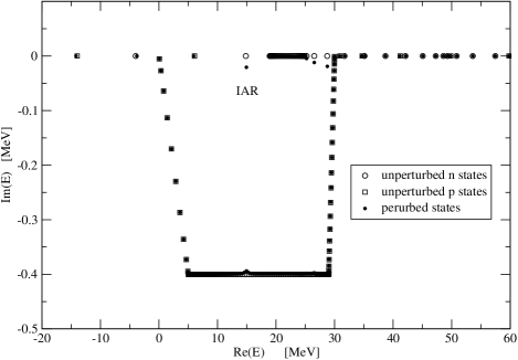
Figure 2: Positions of the $g_{9/2}$ Berggren basis states (circles for neutrons and squares for protons) and the results of the CXSM method (filled circles) on the complex $E$-plane for the Coulomb potential Eq. (30).

To understand better the formation of the IAR let us consider again the $l=4$, $j=9/2$ case as an example. In Fig. 2 we show the positions of the unperturbed states forming the Berggren basis (denoted by circles for neutrons and squares for protons) and some of the results of the diagonalization (perturbed states denoted by filled circles) on the complex energy plane. A section of the real $E$-axis and of the lower half of the complex plane is shown. In this case the neutron contour is along the real axis while the proton contour has a trapezoidal shape with vertexes denoted by LP1 in Table 2. In order to see better the region of our interest the states with energies higher than $60$ MeV are not shown in Fig.2. The discrete basis states are listed in Table 1. The bound basis states are the $1g_{9/2}$ proton state at $E_{i}^{(p)}=-13.975$ MeV and the two neutron states: $1g_{9/2}$, $2g_{9/2}$ at $E_{i}^{(n)}=-22.878$ MeV and at $E_{i}^{(n)}=-4.060$ MeV which are shifted up by $\Delta_{c}=18.9$ MeV . The narrow $2g_{9/2}$ proton resonance at $E_{i}^{(p)}=(6.070,-2\times 10^{-5})$ MeV seems to lie on the real axis.

$l~{}j$	$E_{r}(CXSM)$	$E_{r}(CS)$	$E_{r}(CC)$	$\Gamma(CXSM)$	$\Gamma(CS)$	$\Gamma(CC)$
$g_{9/2}$	14.933	14.933	14.934	0.041	0.041	0.042
$i_{11/2}$	15.493	15.493	15.493	0.002	0.002	0.002
$d_{5/2}$	16.436	16.436	16.444	0.121	0.120	0.120
$s_{1/2}$	16.913	16.913	16.913	0.127	0.127	0.128
$g_{7/2}$	17.350	17.349	17.349	0.076	0.075	0.074
$d_{3/2}$	17.434	17.434	17.433	0.118	0.119	0.120
$j_{15/2}$	18.752	18.751	18.752	0.005	0.005	0.005

Table 4: Comparison of the IAR parameters calculated by using the CC, CXSM and CS methods for different partial waves with the dilatation analytic Coulomb potential Eq. (32). Energies are in MeV units.

Most of the perturbed states lie close to the positions as the corresponding basis states since the coupling symmetry potential term cases only a small shift for these states. One of the exception is the IAR at ${\cal E}_{IAR}=(14.933,-0.021)$ MeV which shifted down well below the bound $2g_{9/2}$ neutron state which is the main component of its wave function $C^{(n)}_{i}=(0.9921,-0.0047)$. The second largest component is that of the $2g_{9/2}$ proton resonance with $C^{(p)}_{i}=(-0.1194,0.0002)$. The other perturbed states which do not fit to the path of the contours are states based on contour states but fall off the contour because of the finite number of discretization points. If the number of discretization points are increased they move closer to the contour. They move also with the contour if we change the shape of the contour in contrast to the IAR which remains in the same position. Of course the IAR should lie above the proton contour in order to be explored. This feature is very similar to the one observed in the CS calculation.

From the mathematical theory of the complex scaling ABC1 ; ABC2 ; ABC3 ; ho83 ; moi98 it is known that the continuous part of the spectrum of the complex scaled Hamilton operator consist of half lines on the complex energy plane. The half lines start at the thresholds and they are rotated down from the real axis by $2\theta$. In our calculation we have used $M_{p}=M_{n}=100$ basis functions and received two hundred approximate complex eigenvalues from the diagonalization. These eigenvalues are plotted on Fig. 3 for two different $\theta$ values $\theta=2^{o}$ and $\theta=4^{o}$. From this Figure it is obvious that the vast majority of the eigenvalues correspond to discretization of the continuous spectrum. However there are a few eigenvalues which are independent from the complex scaling parameter $\theta$. These are denoted by letters $b_{1}$,$b_{2}$ and $r_{1}$,$r_{2}$ in the Figure 3. The $r_{2}$ is the IAR which is based mainly on the $2g_{9/2}$ bound neutron state as we have seen in the CXSM calculation before. The $r_{1}$ resonance is based mainly on the narrow $2g_{9/2}$ proton resonance at $E_{i}^{(p)}=(6.070,-2\times 10^{-5})$ MeV. The bound states $b_{1}$ and $b_{2}$ originate on the $1g_{9/2}$ proton state at $E_{i}^{(p)}=-13.975$ MeV and the $1g_{9/2}$ neutron state at $E_{i}^{(n)}=-22.878$ MeV which are shifted up by $\Delta_{c}=18.9$ MeV.

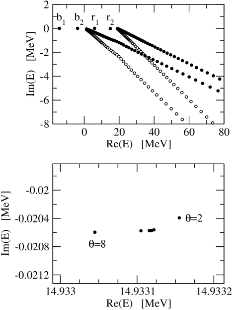
Figure 3: Upper part: positions of the $g_{9/2}$ states on complex $E$-plane with CS method with the rotation angle $\theta=2^{o}$ (filed circles) and with $\theta=4^{o}$ ( open circles) for the Coulomb potential Eq. (32). The IAR is the state $r_{2}$. Lower part: the vicinity of the IAR, the CS scaling parameter $\theta$ is varied between $2^{o}$ and $8^{o}$ with a step size of $1^{o}$.

The lower part of the Figure 3 show the so called $\theta$ trajectory i.e. the complex energy plane in the vicinity of the IAR when the complex scaling parameter changes between $\theta=2$ and $\theta=8$ degrees with step size of one degree. There is a small change in the position and width of the resonance (this should be independent form the value of $\theta)$ but this comes from the fact that a finite basis is used. This phenomena is well know in all complex scaling calculation and there are methods how to select the best approximation for the resonance yar78 . The resonance position and width values given in Table 4 correspond to calculations with $\theta=4^{o}$.

A similarity of the CXSM and the CS method is that results become less accurate if the contour of the CXSM or the rotated half lines are lying close to the resonance. To get high accuracy the resonance has to be well explored i.e. should lie far above the contour. The rotated half lines of the CS play similar role as the contours of the CXSM therefore we shall call the half lines of the CS method also contours. Only the resonances above the contours can be calculated. This means that the $3g_{9/2}$ neutron resonance at $E^{(n)}=(4.929,-6.035)$ $\arg(E^{(n)})=50.76^{o}$ or the corresponding perturbed solution can not be calculated by the CS method since they can not be explored due to the critical angle of the WS potential $\theta_{crit}=18.48^{o}$. It can be calculated however by the CXSM using contours $LP3-LN3$ and we get for the perturbed energy ${\cal E}_{p}=(23.996,-6.147)$ MeV $\arg({\cal E}_{p}-\Delta_{c})=50.33^{o}$.

The similarity of the methods can be seen even better if we try to use a contour in CXSM, which resembles to the rotated continuum of the CS calculation. In Fig. 4 we present the results of the CXSM calculation in which the contours LP2 and LN2 were chosen to be the same as the one corresponding to the optimal $\theta=4^{o}$ rotational angle of the CS calculation. One can see that the IAR is well separated from the two contours starting at the origin and the one starting at the neutron emission threshold. The unperturbed pole closest to the IAR is the bound $2g_{9/2}$ neutron state which is the dominating component of the IAR wave function with amplitude: $C^{(n)}_{i}=(0.9918,-0.0043)$. The second largest component of the IAR wave function is the one of the $2g_{9/2}$ proton resonance with amplitude $C^{(p)}_{i}=(-0.1194,0.0001)$. The wave function of the IAR practically unchanged as far as the discrete components are concerned with respect to the case with the contours used in Fig. 2 (LP1 and a real neutron contour). The energy of the IAR is ${\cal E}_{p}=(14.93309,-0.02058)$ MeV coincide with the one ${\cal E}_{p}=(14.93303,-0.02062)$ MeV with the contours used in Fig. 2 within the numerical error $1$ keV estimated from the deviation from the CC results in Table 4. This good agreement convinces us that the use of the LP2 and LN2 contours which resembles to the contour of the CS could also be used for calculating the IAR. The components of the different scattering states taken from the different contours are certainly very different but the summed contribution of the proton and neutron contours are basically the same. Since both are small numbers their numerical values have little importance. For the $g_{9/2}$ IAR the neutron continuum has negligible effect. For other partial waves this effect is also small but not completely negligible.

An important difference between the results presented in Figs. 3 and 4 is that in Fig. 3 only perturbed states are shown since in the CS method the basis states used are not eigenstates of any unperturbed Hamiltonians. Therefore from the coefficients of the wave function of the IAR explored we can not estimate the role of the unperturbed neutron and proton states easily. To get similar quantities we have to calculate the unperturbed state with the same CS contour and we have to calculate overlaps with the IAR wave function.

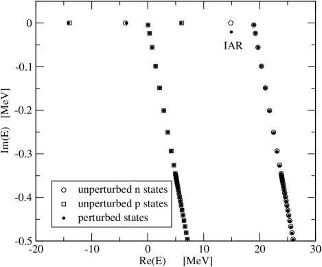
Figure 4: Positions of the $g_{9/2}$ Berggren basis states (circles for neutrons and squares for protons) and the results of the CXSM method (filled circles) on the complex $E$-plane for the Coulomb potential Eq. (32) with contours LP2 and LN2 in Table 2. They are similar to the optimal contour of the CS method.

IV Summary

Let us summarize briefly the results we received in this study. We reproduced the results of the direct numerical solution of the coupled Lane equations by diagonalizing the Hamiltonian in the full n-p Berggren basis i.e. using the CXSM method. The IAR parameters were extracted from the $S({\cal E}_{p})$ calculated by solving the Lane equation along the real ${\cal E}_{p}$-axis by fitting it using the one pole approximation Eq. (31). The fitted position $E_{r}(CC)$ and the width $\Gamma(CC)$ of the IAR was compared to the result of the CXSM calculation and the agreement was generally better than 1 keV for all partial waves in which we had IAR. In the wave function of the IAR furnished by the CXSM the contribution of the bound neutron state has the dominant role and the proton resonance has a non negligible effect. The integrated effect of the proton continuum is small but essential to produce the correct width for the resonance. We studied the details of the different parts of the continuum segments and the necessary numbers of the discretization points on the different segments. The role of the cut off energy and the low energy part of the continuum were also investigated. The neutron continuum played very small effect for the IAR-es.

The pole position of the IAR was calculated by complex scaling method as well. For that we modified the Coulomb potential for a dilatational analytic one and repeated the CC calculation and CXSM method with the modified Coulomb potential. We received very good agreement to the numerical solution of the coupled Lane-equations both with the CXSM and the CS methods. Therefore we conclude that in this case the CXSM and the CS method give basically the same results apart some numerical errors which naturally not the same in the two type of calculations. This agreement suggests that the two method are basically equivalent in those cases when both methods can be applied.

Besides the similarities and differences of the CXSM and the CS methods discussed so far there are further important differences between them. The application of the uniform CS method used here is restricted to dilatation analytic potentials and the range of the rotational angle could also be limited. On the other hand in the CXSM method the shape of the contour can be chosen with large flexibility although to go too deep into the complex energy might spoil a bit the accuracy of the calculated results. Another advantage of the CXSM is that the structure of the resonant state can be seen directly from the coefficients of the perturbed wave function. In the CS method the same information can be explored in a more indirect way.

- (1) T. Teranishi et al., Phys. Lett. B407, 110 (1997).
- (2) S. Takeuchi et al., Phys. Lett. B515, 255 (2001).
- (3) G.V. Rogachev et al., Phys. Rev. C 67, 041603(R) (2003).
- (4) G.V Rogachev et al., Phys. Rev. Lett. 92, 232502 (2004).
- (5) R. Id Betan, R. J. Liotta, N. Sandulescu and T. Vertse, Phys. Rev. Lett. 89, 042051 (2002).
- (6) R. Id Betan, R. J. Liotta, N. Sandulescu and T. Vertse, Phys. Rev. C 67, 014322 (2003).
- (7) N. Michel, W. Nazarewicz, M. Ploszajczak and K. Bennaceur, Phys. Rev. Lett. 89, 042052 (2002).
- (8) N. Michel, W. Nazarewicz, M. Płoszajczak and J. Okołowicz, Phys. Rev. C 67, 054311 (2003).
- (9) N. Michel, W. Nazarewicz, and M. Płoszajczak, Phys. Rev. C 75, 031301(R) (2007).
- (10) N. Michel, W. Nazarewicz, and M. Płoszajczak, Nucl. Phys. A794, 29 (2007).
- (11) J. Rotureau, N. Michel, W. Nazarewicz, M. Płoszajczak, and J. Dukelsky, Phys. Rev. Lett. 97, 110603 (2006).
- (12) T. Berggren, Nucl. Phys. A109, 265 (1968).
- (13) R. Id Betan, N. Sandulescu, and T. Vertse, Nucl. Phys. A771, 93 (2006).
- (14) G. G. Dussel, R. Id Betan, R. J. Liotta, T. Vertse, Nucl. Phys.A789, 182 (2007).
- (15) T. Vertse, R. J. Liotta, E. Maglione, Nucl. Phys. A584, 13 (1995).
- (16) J. Blomqvist, O. Civitarese, E.D. Kirchuk, R. J. Liotta, and T. Vertse, Phys. Rev. C 53, 2001 (1996).
- (17) R.J. Liotta, E. Maglione, N. Sandulescu, T. Vertse, Phys. Letters 367, 1 (1996).
- (18) J. Aguilar, J. M. Combes, Commun. Math. Phys 22, 269 (1971).
- (19) E. Balslev, J. M. Combes, Commun. Math. Phys 22, 280 (1971).
- (20) B. Simon, Commun. Math. Phys 27, 1 (1971).
- (21) Y.K. Ho, Phys. Rep. 99, 1 (1983).
- (22) N. Moiseyev, Phys. Rep. 302, 211 (1998).
- (23) A.M. Lane, Nucl. Phys. A35, 676 (1962).
- (24) G. Colo, H. Sagawa, N. Van Giai, P.F. Bortignon and T. Suzuki, Phys. Rev. C 57, 3049 (1998).
- (25) R. F. Barett, B. A. Robson, W. Tobocman, Rev. Mod. Phys. 55, 155 (1983).
- (26) T. Myo, A. Ohnishi, and K. Katō, Prog. Theor. Phys. 99, 801 (1998).
- (27) G. Hagen and J.S. Vaagen, Phys. Rev. C 73, 034321 (2006).
- (28) N. Michel, W. Nazarewicz, and M. Płoszajczak, Phys. Rev. C 70, 064313 (2004).
- (29) R. Id Betan, R. J. Liotta, N. Sandulescu, T. Vertse and R. Wyss, Phys. Rev. C 72, 054322 (2005).
- (30) N. Michel, W. Nazarewicz, M. Płoszajczak, J. Rotureau, Phys. Rev. C 74, 054305 (2006).
- (31) Ya. B. Zel’dovich, Zh. Eksp. i Theor. Fiz. 39, 776 (1960).
- (32) W. J. Romo, Nucl. Phys. A116, 617 (1968).
- (33) B. Gyarmati and T. Vertse, Nucl. Phys. A160, 523 (1971).
- (34) B. Gyarmati and T. Vertse, Nucl. Phys. A182, 315 (1972).
- (35) J. Toulouse, Phys. Rev. B 72, 035117 (2005).
- (36) S. Saito, Suppl. Prog. Theor. Phys. 62, 11 (1977).
- (37) D. Baye, M. Hesse and M. Vincke, Phys.Rev. E 65, 026701 (2002).
- (38) D. Baye and P.-H. Heenen, J. Phys. A19, 2041 (1986).
- (39) D. Baye, Nucl. Phys. A627, 305 (1997).
- (40) R. Yaris and P. Winkler, J. of Phys. B11, 1475 (1978).