Superconducting pumping of nanomechanical vibrations

Abstract

We demonstrate that a supercurrent can pump energy from a battery that provides a voltage bias into nanomechanical vibrations. Using a device containing a nanowire Josephson weak link as an example we show that a nonlinear coupling between the supercurrent and a static external magnetic field leads to a Lorentz force that excites bending vibrations of the wire at resonance conditions. We also demonstrate the possibility to achieve more than one regime of stationary nonlinear vibrations and how to detect them via the associated dc Josephson currents and we discuss possible applications of such a multistable nanoelectromechanical dynamics.

Coupling of electronic and mechanical degrees of freedom on the nanometer length scale is the basic phenomenon behind the functionality of nanoelectromechanical (NEM) systems. Such a coupling can be mediated either by electrical charges or currents. Single-electron tunneling (SET) devices with movable islands or gate electrodes employ Coulomb forces to achieve capacitive Naik et al. (2006); Knobel and Cleland (2003) and shuttle NEM coupling Gorelik et al. (1998); Shekhter et al. (2007), where the latter involves both capacitive forces and charge transfer. Devices containing current carrying parts, on the other hand, will achieve NEM coupling through magnetic-field induced Lorentz forces. Focusing on the latter mechanism, a simple estimate shows that for a gold nanowire suspended over a few micrometer long trench, the mechanical displacement due to typical currents of order 100 nA in magnetic fields of order 0.01 T can be as large as one nanometer. Such displacements can crucially affect the performance of mesoscopic devices.

In this Letter we will explore a possible scenario for how highly nonlinear nanoelectromechanical effects can arise if the magnetic-field induced electromotive force caused by the mechanical motion of a conducting wire strongly perturbs the flow of current through it. Devices which contain superconductors, with their known extreme sensitivity to external electric fields, are the best candidates to achieve such strong effects and superconducting quantum interference devices (SQUID’s) that incorporate a nanomechanical resonator are particularly interesting. Significant research has recently been performed in this direction (see e.g Ref. Buks and Blencowe, 2006; Buks et al., 2008; Blencowe and Buks, 2007; Zhou and Mizel, 2006), by using a coupling between the SQUID dynamics and the resonator’s mechanical vibrations due to the constraint set by the flux quantization phenomenon. Here we will consider the new possibility for NEM coupling that occurs if the nanomechanical element is an integral part of the superconducting weak link. In this case the NEM vibrations directly affect the Cooper pair tunneling and significantly modify the properties of the link. With a voltage biased weak link it becomes possible to pump nanomechanical vibrations in the Cooper pair tunneling region. As we will show below the result is a peculiar nonlinear NEM dynamics that affect both the supercurrent flow and the nanomechanical vibrations in novel ways.

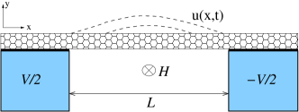
Figure 1: (Color online) Sketch of system considered. A nanowire is suspended between two superconducting electrodes separated by a trench of length $L$. When the system is biased by a voltage $V$, the Lorentz force caused by the coupling of the Josephson current and a transverse magnetic field, $H$, induces wire vibrations described by the coordinate $u(x,t)$. The nonlinear coupling leads to a multistability of the system resulting in different dc Josephson current regimes (see text).

The Hamiltonian describing the electronic subsystem in the specific model system shown in Fig. 1 reads,

$$\hat{\mathcal{H}}=\int\textrm{d}x\hat{\Psi}^{\dagger}(x)\left(\hat{\mathcal{H}}_{0}+\hat{\mathcal{H}}_{\Delta}\right)\hat{\Psi}(x)$$

$$\hat{\mathcal{H}}_{0}=-\frac{\hbar^{2}}{2m}\sigma_{z}\left(\frac{\partial}{\partial x}-\sigma_{z}\frac{ieHu(x,t)}{\hbar}\right)^{2}+\sigma_{z}U(x)$$ (1)

$$\hat{\mathcal{H}}_{\Delta}=\Delta(x)\left(\sigma_{x}\cos\phi(t)+\text{sign}(x)\sigma_{y}\sin\phi(t)\right)\,,$$

where $\Psi^{\dagger}(x)$ [$\Psi(x)$] are two-component Nambu-spinors and $\sigma_{i}$ are the Pauli matrices in Nambu space . The deflection of the tube is given by $u(x,t)=u(x)a(t)$, where $u(x)$ is the normalized (dimensionless) profile of the fundamental bending mode and $a(t)$ determines its amplitude; other modes are less important and will be ignored. The potential $U(x)$ describes the barrier between the nanowire and the bulk superconducting electrodes, where the gap parameter is $\Delta(x)=\Delta_{0}\theta(2|x|-L)$ with $\Delta_{0}\sim$10 meV. The phase difference across the junction due to the bias voltage $V$ is $\phi(t)=2eVt/\hbar$.

A convenient gauge transformation, see Ref. Shekhter et al., 2006 for a similar analysis, shifts the vector potential induced by the nanotube deflection from the kinetic part of the Hamiltonian to the phase difference between the leads, so that $\phi(t)\rightarrow\varphi(t)=\phi(t)-a(t)4eH\int_{0}^{L/2}u(x)\text{d}x/\hbar$. In the adiabatic limit, $\hbar D\dot{\varphi}(t)\ll\Delta_{0}$, with $D$ the transparency of the barriers, one can then evaluate the fixed-phase ground state energy of the electronic subsystem Bagwell (1992) as $E(\varphi)=-\Delta_{0}[1-D\sin^{2}(\varphi/2)]^{1/2}$, and find that the force exerted on the wire, $F=-\partial E(\varphi(a))/\partial a$, is proportional to the Josephson current $j=(2e/\hbar)\partial E(\varphi)/\partial\varphi$. The resulting effective equation of motion for the nanowire vibrating in its fundamental bending mode describes a forced nonlinear oscillator with damping. In terms of the dimensionless coordinate $Y(t)=[4eLH/\hbar]a(t)$ one finds in the low transparency limit, $D\ll 1$, the result

$$\ddot{Y}+\tilde{\gamma}\dot{Y}+Y=\epsilon\sin(\varphi)$$ (2a)

$$\dot{\varphi}=\widetilde{V}-\dot{Y}\,.$$ (2b)

Here, $\tilde{\gamma}=\gamma/m\omega$ is a dimensionless damping coefficient, while $\epsilon=8eL^{2}H^{2}j_{c}/(m\hbar\omega^{2})$ is the amplitude and $\dot{\varphi}$ the frequency of the driving force with $\widetilde{V}=2eV/(\hbar\omega)$, $\omega$ the mechanical eigenfrequency, $m$ the mass of the nanowire, $j_{c}=D\Delta_{0}e/(2\hbar)$ the critical current and time $t$ measured in units of $1/\omega$. In (2a), the driving force on the nanowire is naturally interpreted as the Lorentz force due to the coupling between the Josephson current and the magnetic field, which, due to the confined geometry of the charge carriers in the nanowire, is responsible for depositing energy from the electronic to the mechanical subsystem. According to (2b), the phase difference $\varphi$ between the leads evolves in time under the influence of both the bias voltage and the electromotive force induced by the motion of the wire in the static magnetic field.

Multiplying (2a) with $\dot{Y}$ and averaging over time we find (using the definition of the Josephson current above) that in the stationary regime the dc current through the system is

$$j_{dc}=\frac{\gamma\langle\dot{a}(t)^{2}\rangle}{V}=\frac{\gamma\hbar^{2}\omega^{2}\langle\dot{Y}(t)^{2}\rangle}{16e^{2}L^{2}H^{2}V},$$ (3)

where $\langle...\rangle$ denotes time-averaged quantities.

To proceed with our analysis we consider the specific case of a single-wall carbon nanotube wire of diameter 1 nm suspended over a length $L\sim$ 1 $\mu$m. With $j_{c}\sim$ 100 nA Kasumov et al. (1999) one then finds that $\epsilon\sim$ 3$\times$10^-3 in a magnetic field of $H\sim$ 20 mT. Since $\tilde{\gamma}=1/Q$, where the quality factor $Q\sim 1000$ Witkamp et al. (2006); Sazonova et al. (2004), both $\epsilon$ and $\tilde{\gamma}$ may be considered small, $\epsilon,\tilde{\gamma}\ll 1$.

Numerical simulations of the nanowire dynamics using the equation of motion (2) with initial conditions $Y(0)=\dot{Y}(0)=0$ show distinct resonance peaks in the vibration amplitude at integer values of $\widetilde{V}$. Figure 2, e.g. shows peaks at $\tilde{V}$=1 and 2 (as well as a small peak at $\widetilde{V}=1/2$), where the onset of the $\widetilde{V}$=2 peak depends on the ratio $\epsilon/\tilde{\gamma}$ .

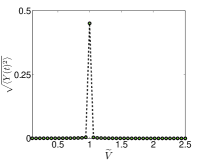
(a) $\,\,\,\epsilon=0.001$

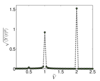
(b) $\,\,\,\epsilon=0.01$

Figure 2: (Color online) Time average of the rms nanowire deflection coordinate $Y(t)$ from a numerical simulation of Eq. (2) as a function of bias voltage $\tilde{V}$ for different force parameters $\epsilon$ ($\tilde{\gamma}=0.001$).

For small vibration amplitudes, when one can expand $\sin(\widetilde{V}t-Y)$ to linear order in $Y$, these results can readily be attributed to a direct resonance at $\tilde{V}=1$ and a parametric resonance at $\widetilde{V}=2$. In this limit there is a resemblance between the resonances in our system and the familiar Fiske effect in Josephson junctions coupled to an electromagnetic resonator Barone and Paterno (1982). However, as can be seen in Fig. 2(b), the oscillation amplitude is too large for the linear approximation to hold if the driving force is large, $\epsilon>\tilde{\gamma}$. As will be shown below, the resonances in this nonlinear regime are significantly different from those of the Fiske effect and demonstrate a variety of unusual peculiarities which could be useful for device applications.

To analyze the nonlinear regime in the vicinity of the resonance peaks it is convenient to apply perturbation theory and expand in the small parameters $\epsilon$ and $\tilde{\gamma}$. With this in mind, it is useful to write the dimensionless deflection coordinate $Y(t)$ of the nanowire as

$$Y(t)=\sqrt{I_{n}(t)}\sin\left(\frac{\widetilde{V}t}{n}+\frac{\chi_{n}(t)}{n}\right),$$ (4)

where the amplitude $A_{n}(t)\equiv\sqrt{I_{n}(t)}$ and phase $\chi_{n}(t)$ vary slowly in time; $\dot{I}_{n}(t),\dot{\chi}_{n}(t)\approx\tilde{\gamma},\epsilon\ll 1$. Substituting this Ansatz into (2) and integrating over the fast oscillations one gets two coupled equations for $I_{n}(t)$ and $\chi_{n}(t)$,

$$\dot{I}_{n}=-\tilde{\gamma}I_{n}-2\epsilon nJ_{n}(\sqrt{I_{n}})\sin\chi_{n}$$ (5a)

$$\dot{\chi}_{n}=-\delta-2\epsilon nJ^{\prime}_{n}(\sqrt{I_{n}})\cos\chi_{n}\,.$$ (5b)

Here, $J_{n}$ are Bessel functions of order $n$, $J^{\prime}_{n}(\sqrt{I_{n}})=dJ_{n}(\sqrt{I_{n}})/dI_{n}$ and $\delta=\widetilde{V}-n$. Stationary nonlinear oscillation regimes can now be found by studying the stationary points of (5) in terms of the system parameters.

We start our analysis by considering the case of exact resonance, $\delta=0$, for which Eq. (5) guarantees that a stationary solution given by $I_{n}=0$ always exists. However, since $J_{n}(x)\sim x^{n}$ for small $x$, one immediately finds that this solution is unstable for $n=1$ (resonance excitation), while for $n=2$ (parametric excitation) it is only unstable if $\epsilon>2\tilde{\gamma}$. This turns out to be the main difference between the two resonance types; the corresponding finite-amplitude stationary regimes are qualitatively very similar. In the following analysis we will therefore focus on the parametric resonance at $n=2$, and omit the index $n$ on amplitudes, phases and Bessel functions.

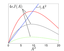
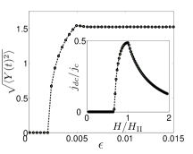
Figure 3: (Color online) (a) Plots for solution of Eq. (5a) with $\dot{I}_{n}=0$ for $\chi_{n}=3\pi/2$ (type-$\mathrm{I}$ regime) and $\epsilon=0.005$ (red solid/dark gray), $\epsilon=0.003$ (black dashed) and $\epsilon=0.001$ (green dashed dotted/light gray). Crossings with the straight line correspond to stationary points. (b) Numerical solution on resonance of Eq. (2) for the time-averaged rms nanowire deflection coordinate as a function of $\epsilon$. Inset shows corresponding plot for dc current as a function of magnetic field. $\delta=0$ and $\tilde{\gamma}=0.001$ throughout.

From Eq. (5b) it is evident that exactly on resonance a finite-amplitude stationary regime may be realized either by fixing the phase, $\cos\chi=0$, or the amplitude, $J^{\prime}(A)=0$. We will refer to these different regimes as type $\mathrm{I}$ and type $\mathrm{II}$. From (5a) it follows that a type-$\mathrm{I}$ stationary point exists for any $\epsilon>\epsilon_{\mathrm{I}}\equiv 2\tilde{\gamma}$. The oscillation amplitude is implicitly given by the equation $\tilde{\gamma}/\epsilon=4J(A_{\mathrm{I}})/A_{\mathrm{I}}^{2}$, which always has a solution in the relevant range of parameters, see Fig. 3 . Furthermore, type-$\mathrm{II}$ stationary points corresponding to fixed-amplitude oscillations, $A_{\mathrm{II}}=A_{0}$, where $J^{\prime}(A_{0})=0$, only exists if $\epsilon>\epsilon_{\mathrm{II}}\equiv\tilde{\gamma}A^{2}_{0}/4J(A_{0})$. In this case there exists two stationary points of equal amplitude, $A_{\mathrm{II}}^{\pm}=A_{0}$, but different phases, $\chi_{\mathrm{II}}^{\pm}=3\pi/2\pm\arccos(\epsilon_{\mathrm{II}}/\epsilon)$ .

A stability analysis shows that the type-I stationary point is stable if $\epsilon<\epsilon_{\mathrm{II}}$, but unstable (a saddle point) for $\epsilon>\epsilon_{\mathrm{II}}$. The type-II stationary points, on the other hand, are always stable if they exist, i.e. when $\epsilon>\epsilon_{\mathrm{II}}$. This means that if one increases $\epsilon$, by turning up the magnetic field, the nanotube vibration amplitude will be zero (to an accuracy of order $\epsilon,\tilde{\gamma}$) until $\epsilon\sim\epsilon_{\mathrm{I}}$. As $\epsilon$ is varied from $\epsilon_{\mathrm{I}}$ to $\epsilon_{\mathrm{II}}$ the amplitude increases from 0 to $A_{0}$, where it saturates as we increase the magnetic field further. This analysis, which also explains the onset of the second peak in Fig. 2(b), has been fully confirmed by numerically solving the equation of motion (2) for the vibration amplitude at varying values of $\epsilon$, as shown in Fig. 3. The inset shows the dc current as a function of magnetic field, where $H_{\mathrm{II}}$ is defined from $\epsilon_{\mathrm{II}}\propto H_{\mathrm{II}}^{2}$ as above. As the dc current scales as $j_{dc}\propto\langle\dot{Y}(t)^{2}\rangle/H^{2}$ one finds that the current initially grows with increasing magnetic field strength, pumping energy into the nanoscale vibrations, but falls off as $1/H^{2}$ once $H>H_{\mathrm{II}}$ and the vibration amplitude has saturated at $A_{0}$.

Moving off the resonance, $\delta$ becomes non-zero and if $\epsilon>\epsilon_{\mathrm{II}}$ the degeneracy of the amplitudes $A_{\mathrm{II}}^{\pm}$ at the type-$\mathrm{II}$ stationary points is lifted. If $\delta>0$ the amplitude $A_{\mathrm{II}}^{+}(\delta)$ is larger and $A_{\mathrm{II}}^{-}(\delta)$ smaller than the on-resonance value $A_{0}$, as shown in Fig. 4, while if $\delta<0$ the opposite is true.

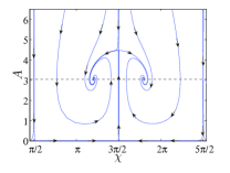
(a) $\,\,\,\delta=0$

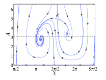
(b) $\,\,\,\delta=2.5\times 10^{-4}$

Figure 4: (Color online) Phase space diagrams in the type-$\mathrm{II}$ regime with $\epsilon=0.01$ and $\tilde{\gamma}=0.001$ showing (a) two asymptotically stable points with vibration amplitude $A_{0}\sim 3$ [dashed line] and (b) their shifts from $A_{0}$ off resonance.

As the degeneracy is lifted, the stable type-$\mathrm{II}$ stationary point that moves to higher amplitudes merges with the type-$\mathrm{I}$ saddle point and disappears at some critical value $\pm\delta_{c}$. Consequently, in the interval $(-\delta_{c},\delta_{c})$ there are two different stable nonlinear regimes ($\pm$) characterized by different nanotube oscillation amplitudes and as a consequence by different dc currents through the system. A detailed analysis shows that if $\epsilon-\epsilon_{\mathrm{II}}<<\epsilon_{\mathrm{II}}$ the width $2\delta_{c}$ of this window of bistability is $\propto(\epsilon-\epsilon_{\mathrm{II}})^{3/2}$, while the maximum difference in amplitudes $|A_{\mathrm{II}}^{+}(\pm\delta_{c})-A_{\mathrm{II}}^{-}(\pm\delta_{c})|$ is $\propto(\epsilon-\epsilon_{\mathrm{II}})$.

The stationary point that describes the system in a particular situation depends on the initial conditions. If initially $A\approx 0$, the system always moves to the stationary point with lowest amplitude as the parametric resonance develops, i.e. $A_{\mathrm{II}}^{-}$ if $\delta>0$ and $A_{\mathrm{II}}^{+}$ if $\delta<0$. However, if the system starts from inside the separatrix defining the higher than on-resonance stationary point (see Fig. 4), it will achieve a stationary amplitude that is larger than on resonance. Alternatively, the system can reach this point if the voltage is slowly changed from resonance, as the system will follow the trajectory of the stationary point at which it is defined exactly on resonance. This represents a unique sensitivity in our system to small changes in the applied bias voltage. Since the dc current through the system depends on the vibration amplitude, $j_{dc}\propto A^{2}$, it follows that we can predict a non-single valued $I-V$ curve close to resonance. The result is a hysteretic behavior, the origin of which lies in the multistability of the pumped nanomechanical vibrations. This means that the magnitude of the dc Josephson current in our device is sensitive to the pumping history. Such memory effects may be employed for different device applications where the sensitivity of the nanomechanical initial conditions and the possibility to switch the system between two stable regimes of vibration can be employed for both sensing and memory devices. As an example we discuss briefly below how a memory device could work.

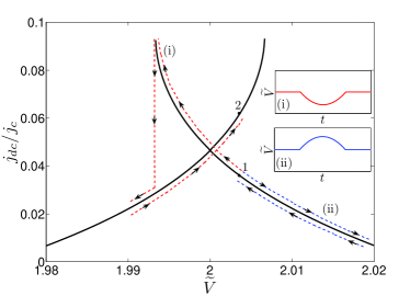
Figure 5: (Color online) Diagram illustrating how small voltage pulses switch the dc Josephson current. The two pulses in the inset have different effects. After pulse (ii) (blue) the current is the same as before, while pulse (i) (red) switches the current by a measurable amount (from point 1 to 2) thereby storing one bit of retrievable information in the device ($\epsilon=0.05$, $\tilde{\gamma}=0.001$).

A scheme for the electrical manipulation of our superconducting nanovibrator is presented in Fig. 5, where the starting position 1 corresponds to a bias voltage which is slightly off resonance and a nanowire that oscillates with an amplitude $A_{\mathrm{II}}^{-}(\delta>0)$ smaller than on resonance, see Fig. 4(b). Now consider the effect of the voltage pulses (i) and (ii) shown in the inset. Pulse (i) moves the system along trajectory (i) to where the vibration amplitude $A_{\mathrm{II}}^{-}(\delta<0)$ is larger than on resonance. However, at $\delta=-\delta_{c}$ this asymptotically stable point merges with the third stationary point (saddle) and becomes unstable. The system therefore jumps to the second asymptotically stable point, where the vibration amplitude $A_{\mathrm{II}}^{+}(\delta<0)$ is smaller than on resonance. When the voltage is increased again, the system will move to position 2, where the vibration amplitude $A_{\mathrm{II}}^{+}(\delta>0)$ and hence the dc current is larger than at position 1. One concludes that pulse (i) writes one bit of information, which is stored as a measurably larger dc current. Pulse (ii), on the other hand, moves the initial stability point back and forth along trajectory (ii) and returns it to the initial position 1. For the parameters considered here, i.e. a resonance frequency of the order 1 GHz, we find that the difference in the current between points 1 and 2 is a few nA. Also, the window of bistability $2\delta_{c}$ is about 50 nV with the second resonance peak $\widetilde{V}=2$ corresponding to an absolute bias voltage of $V\sim$ 5 $\mu$V. The corresponding mid-point amplitude of vibration of the nanowire is $\sim$ 25 nm.

It is interesting to again compare the phenomena discussed in this Letter with the Fiske effect Barone and Paterno (1982). Repeating our analysis we find the low-amplitude behavior to be similar for the two systems. However, we predict that a dynamical multistability will appear at a certain value, $\epsilon_{\mathrm{II}}$, of the driving Lorentz force. This does not occur in the Fiske effect, where the vibration amplitude exactly on resonance follows the stable solution corresponding to $\cos\chi=0$ in (5b) for all driving forces $\epsilon$.

To conclude we have shown that for a nanowire suspended between two voltage-biased superconducting electrodes in a transverse magnetic field, pronounced resonance phenomena can be found at discrete values of the driving voltage. Our analysis shows that the behavior of this system is governed by an effective equation of motion whose solution gives the amplitude of the nanowire oscillations and the dc Josephson current as a function of system parameters. Most importantly, it was shown that for realistic experimental parameters the system can be driven into a multistable regime by varying the magnetic field strength. The possibility to pump energy into the mechanical vibrations of a suspended nanowire and the ensuing dynamical multistability of the vibration amplitude and dc current makes this superconducting nanoelectromechanical device a unique system, where the sensitivity to initial conditions and switching between two stable regimes can be probed experimentally.

Financial support from the Swedish VR and SSF is gratefully acknowledged.

References

- Naik et al. (2006) A. Naik, O. Buu, M. D. LaHaye, A. D. Armour, A. A. Clerk, M. P. Blencowe, and K. C. Schwab, Nature 443, 193 (2006).
- Knobel and Cleland (2003) R. G. Knobel and A. N. Cleland, Nature 424, 291 (2003).
- Gorelik et al. (1998) L. Y. Gorelik, A. Isacsson, M. V. Voinova, B. Kasemo, R. I. Shekhter, and M. Jonson, Phys. Rev. Lett. 80, 4526 (1998).
- Shekhter et al. (2007) R. I. Shekhter, R. I. Gorelik, M. Jonson, Y. M. Garpelin, and V. M. Vinokur, J. Comput. Theor. Nanos. 4, 860 (2007).
- Buks and Blencowe (2006) E. Buks and M. P. Blencowe, Phys. Rev. B 74, 174504 (2006).
- Buks et al. (2008) E. Buks, E. Segev, S. Zaitsev, B. Abdo, and M. P. Blencowe, Europhys. Lett. 81, 10001 (2008).
- Blencowe and Buks (2007) M. P. Blencowe and E. Buks, Phys. Rev. B 76, 014511 (2007).
- Zhou and Mizel (2006) X. Zhou and A. Mizel, Phys. Rev. Lett. 97, 267201 (2006).
- Shekhter et al. (2006) R. I. Shekhter, L. Y. Gorelik, L. I. Glazman, and M. Jonson, Phys. Rev. Lett. 97, 156801 (2006).
- Bagwell (1992) P. F. Bagwell, Phys. Rev. B 46, 12573 (1992).
- Kasumov et al. (1999) A. Y. Kasumov, R. Deblock, M. Kociak, B. Reulet, H. Bouchiat, I. I. Khodos, Y. B. Gorbatov, V. T. Volkov, C. Journet, and M. Bughard, Science 284, 1508 (1999).
- Witkamp et al. (2006) B. Witkamp, M. Poot, and H. S. J. van der Zant, Nano Lett. 6, 2904 (2006).
- Sazonova et al. (2004) V. Sazonova, Y. Yaish, H. Ustunel, D. Roundy, T. A. Arias, and P. L. McEuen, Nature 431, 284 (2004).
- Barone and Paterno (1982) A. Barone and G. Paterno, Physics and applications of the Josephson effect (John Wiley & Sons, 1982), p. 235.