Quantum interference in laser-induced nonsequential double ionization in diatomic molecules: the role of alignment and orbital symmetry

Abstract

We address the influence of the orbital symmetry and of the molecular alignment with respect to the laser-field polarization on laser-induced nonsequential double ionization of diatomic molecules, in the length and velocity gauges. We work within the strong-field approximation and assume that the second electron is dislodged by electron-impact ionization, and also consider the classical limit of this model. We show that the electron-momentum distributions exhibit interference maxima and minima due to the electron emission at spatially separated centers. The interference patterns survive the integration over the transverse momenta for a small range of alignment angles, and are sharpest for parallel-aligned molecules. Due to the contributions of transverse-momentum components, these patterns become less defined as the alignment angle increases, until they disappear for perpendicular alignment. This behavior influences the shapes and the peaks of the electron momentum distributions.

I Introduction

High-order harmonic generation (HHG) or above-threshold ionization (ATI) owe their existence to the recombination, or elastic collision, respectively, of an electron with its parent ion or molecule tstep . Such processes take place within a fraction of a laser cycle, which, for a typical Titanium-Sapphire, high-intensity laser pulse is $T\sim 2.7fs$. Therefore, HHG and ATI occur within hundreds of attoseconds Scrinzi2006 . As a direct consequence, one may use both phenomena to retrieve information from a molecule, in particular the configuration of ions with which the active electron recombines or rescatters, with subfemtosecond and subangstrom precision. Concrete examples include the tomographic reconstruction of molecular orbitals Itatani , and the probing of structural changes in molecules with attosecond precision attomol .

In particular diatomic molecules, due to their simplicity, have attracted a great deal of attention TDSE2005 ; doubleslit ; KB2005 ; KBK98 ; MBBF00 ; Madsen ; Usach2006 ; Usachenko ; HenrikDipl ; Kansas ; PRACL2006 ; moreCL ; DM2006 ; HBF2007 ; F2007 . For such systems, sharp interference maxima and minima in the ATI or HHG spectra have been identified, which could be explained by the fact that harmonic or photoelectron emission took place at spatially separated sites. Therefore, a diatomic molecule may be viewed as the microscopic counterpart of a double-slit experiment doubleslit .

Apart from the above-mentioned phenomena, nonsequential double or multiple ionization, may, in principle, also be employed to extract information about the structure of a molecule. This is not surprising, since laser-induced recollision also plays an important role in this case. The main difference from the previous scenarios is that the returning electron rescatters inelastically with its parent ion, or molecule, giving part of its kinetic energy to release other electrons. In particular, for the simplest case of nonsequential double ionization (NSDI), this may occur through direct, electron-impact ionization, or by excitation-tunneling mechanisms, in which, upon recollision, the first electron excites the second. Thereafter, the second electron tunnels out from an excited state. If more than two electrons are involved, there may exist more complex ionization mechanisms subsequent to recollision. Recently, a statistical thermalization model has been proposed in order to account for these mechanisms and provide a simple description of nonsequential multiple ionization therm2006 .

Specifically for NSDI of molecules, early measurements have already revealed that the total double ionization yields depend on the molecular species, and that there is an intensity region for which the predictions of sequential models break down Cor98 . Furthermore, recent NSDI experiments on diatomic molecules have shown that the shapes of the electron momentum distributions depend on the symmetry of the highest occupied molecular orbital. This holds even if the molecular sample is randomly aligned with respect to the laser-field polarization NSDIsymm . Indeed, in NSDIsymm , very distinct electron momentum distributions have been observed for $N_{2}$ and $\ O_{2}$, as functions of the electron momentum components $p_{n\parallel}$ $(n=1,2)$ parallel to the laser-field polarization. For the former species, elongated maxima along the diagonal $p_{1\parallel}=p_{2\parallel}$ have been reported, while, for $O_{2},$ the distributions exhibit a prominent maximum in the region of vanishing parallel momenta, and are quite broad along the direction $p_{1\parallel}=-p_{2\parallel}+const$. This has been confirmed by theoretical computations within a classical framework, which reproduced some of the differences in the yields.

Subsequently, it has been found that the peak momenta and the shape of the $N_{2}$ electron-momentum distributions changed considerably with the alignment angle of the molecules, with respect to the laser-field polarization NSDIalign . Specifically, for parallel alignment, roughly $40\%$ larger peak momenta along the diagonal $p_{1\parallel}=p_{2\parallel}$ have been observed, as compared to the perpendicular case. Furthermore, for perpendicular alignment, a larger number of events in the second and fourth quadrant of the momentum plane $(p_{1\parallel},p_{2\parallel})$ has been reported. In NSDIalign , these events have been attributed to excitation-tunneling mechanisms.

Despite the above-mentioned investigations, NSDI in molecules has been considerably less studied than HHG or ATI, possibly due to the fact that it is far more difficult to measure, or to model NSDIreview . Solely from a theoretical viewpoint, even for a single atom, it is a very demanding task to perform a fully numerical, three-dimensional computation of NSDI differential electron momentum distributions, for the parameter range of interest. Indeed, only very recently, this has been achieved for Helium RuizBeck , which is the simplest species for which NSDI occurs. An alternative to that are semi-analytical approaches, mostly within the framework of the strong-field approximation (SFA). Such methods are easier to implement and provide a more transparent physical interpretation of the problem. They exhibit, however, several contradictions. A concrete example is the fact that cruder types of electron-electron interaction, such as a contact-type interaction at the position of the ion, lead to a better agreement with the experiments as compared to more refined choices, such as a long-range Coulomb-type interaction FSLB2004 ; FL2005 . Apart from that, it is not clear whether the interference patterns due to electron emission in spatially separated centers survive the integration over the transverse momentum components. This is particularly important, as in most NSDI experiments, these quantities are not resolved.

These issues add up to the already vast amount of open questions related to HHG and ATI in molecules. Indeed, even for these considerably more studied phenomena, topics such as the gauge dependence of the interference patterns PRACL2006 ; DM2006 ; F2007 , the role of different scattering or recombination scenarios KBK98 ; Usach2006 ; PRACL2006 ; HBF2007 ; F2007 , and the influence of collective effects collective or polarization DM2006 ; dressedSFA ; BCM2007 on the electronic bound states have raised considerable debate. Apart from that, specifically for NSDI, it is not even clear if the interference patterns would survive the integration over the transverse electron momenta. This is particularly important, as, in most NSDI experiments, the transverse momenta of the two electrons is not resolved.

In this paper, we perform a systematic analysis of quantum-interference effects in NSDI of diatomic molecules. We work within the strong-field approximation (SFA) and assume that the second electron is dislodged by electron-impact ionization. We also employ the classical limit of this model. We consider frozen nuclei, and the linear combination of atomic orbitals (LCAO approximation). This very simplified model has the main advantage of allowing a transparent picture of the physical mechanisms behind the interference patterns. Specifically, we investigate the influence of the orbital symmetry and of the alignment angle on the NSDI electron momentum distributions, and whether, within our framework, the features reported in NSDIsymm and NSDIalign are observed. Furthermore, we address the question of whether well-defined interference patterns such as those observed in ATI or HHG computations may also be obtained for NSDI, and, if so, under which conditions.

This paper is organized as follows. In Sec. II.1 we briefly recall the expression for the NSDI transition amplitude, which is subsequently applied to diatomic molecules (Sec. II.2). Thereafter, we employ this approach to compute differential electron momentum distributions, for angle-integrated (Sec. III.1), and aligned molecules (Sec. III.2). In the latter case, we analyze the dependence of the interference patterns on the alignment conditions. Finally, in Sec. IV, we state the main conclusions of this paper.

II Transition amplitudes

II.1 General expressions

The simplest process behind NSDI corresponds to the scenario in which the first electron, upon return, releases the second by electron-impact ionization. The pertaining transition amplitude, within the SFA, reads

$$M(\mathbf{p}_{n},t,t^{\prime})=\int_{-\infty}^{\infty}dt\int_{-\infty}^{t}dt^{\prime}\int d^{3}kV_{p_{n}k}V_{k0}e^{iS(\mathbf{p}_{n},\mathbf{k},t,t^{\prime})},$$ (1)

with the action

$$S(\mathbf{p}_{n},\mathbf{k},t,t^{\prime}) = -\sum_{n=1}^{2}\int_{t}^{\infty}\frac{[\mathbf{p}_{n}+\mathbf{A}(\tau)]^{2}}{2}d\tau$$ (2)

$$-\int_{t^{\prime}}^{t}\frac{[\mathbf{k}+\mathbf{A}(\tau)]^{2}}{2}d\tau-E_{02}t-E_{01}t^{\prime}$$

and the prefactors

$$V_{\mathbf{k}0}=<\mathbf{\tilde{k}}(t^{\prime})|V|\phi_{0}^{(1)}>$$ (3)

and

$$V_{\mathbf{p}_{n}\mathbf{k}}=<\mathbf{\tilde{p}}_{1}\left(t\right),\mathbf{\tilde{p}}_{2}\left(t\right)|V_{12}|\mathbf{\tilde{k}}(t),\phi_{0}^{(2)}>.$$ (4)

Eq. (1) describes the physical process in which an electron, initially in a bound state $|\phi_{0}^{(1)}>,$ is released by tunneling ionization at a time $t^{\prime}$ into a Volkov state $|\mathbf{\tilde{k}}(t)>$. Subsequently, this electron propagates in the continuum from $t^{\prime}$ to a later time $t.$ At this time, it is driven back by the field and frees a second electron, which is bound at $|\phi_{0}^{(2)}>,$ through the interaction $V_{12}.$ Finally, both electrons are in Volkov states. The final electron momenta are described by $\mathbf{p}_{n}(n=1,2).$ In the above-stated equations, $E_{0n}$ $(n=1,2)$ give the ionization potentials, and $V$ the binding potential of the system in question. The form factors (3) and (4) contain all the information about the binding potential, and the interaction by which the second electron is dislodged, respectively.

Clearly, $V_{\mathbf{k}0}$ and $V_{\mathbf{p}_{n}\mathbf{k}}$ are gauge dependent. In fact, in the length gauge $\mathbf{\tilde{p}}_{n}\left(\tau\right)=\mathbf{p}_{n}+\mathbf{A}(\tau)$ and $\mathbf{\tilde{k}}(\tau)=\mathbf{k}+\mathbf{A}(\tau)(\tau=t,t^{\prime}),$ while in the velocity gauge $\mathbf{\tilde{p}}_{n}\left(\tau\right)=\mathbf{p}_{n}$ and $\mathbf{\tilde{k}}(\tau)=\mathbf{k}.$ This is a direct consequence of the fact that the gauge transformation $\chi_{l\rightarrow v}=\exp[-i\mathbf{A}(\tau)\cdot\mathbf{r}]$ from the length to the velocity gauge causes a translation $\mathbf{p}\rightarrow\mathbf{p}-\mathbf{A}(\tau)$ in momentum space. This is particularly critical for spatially extended systems, such as molecules, and may alter the interference patterns. A similar effect has also been investigated for high-order harmonic generation dressedSFA ; F2007 and above-threshold ionization DM2006 ; BCM2007 . These discrepancies can be overcome by adequately dressing the electronic bound states, in order to make them gauge equivalent F2007 . In this work, we will restrict ourselves to the field-undressed case. We expect, however, based on the results of F2007 , that the field-dressed velocity gauge distributions will have very similar patterns to the field-undressed length gauge distributions. The same will hold for their dressed length-gauge and the undressed velocity-gauge counterparts.

II.2 Diatomic molecules

We will now consider the specific case of diatomic molecules. For simplicity, we will assume frozen nuclei, the linear combination of atomic orbitals (LCAO) approximation, and homonuclear molecules. Explicitly, the molecular bound-state wave function for each electron reads

$$\psi_{0}^{(n)}(\mathbf{r}_{n})=C_{\psi}\left[\phi_{0}^{(n)}(\mathbf{r}_{n}-\mathbf{R}/2)+\epsilon\phi_{0}^{(n)}(\mathbf{r}_{n}+\mathbf{R}/2)\right]$$ (5)

where $n=1,2,$ $\epsilon=\pm 1$, and $C_{\psi}=1/\sqrt{2(1+\epsilon S(\mathbf{R})}$, with

$$S(\mathbf{R})=\int\left[\phi_{0}^{(n)}(\mathbf{r}_{n}-\mathbf{R}/2)\right]^{\ast}\phi_{0}^{(n)}(\mathbf{r}_{n}+\mathbf{R}/2)d^{3}r.$$ (6)

The positive and negative signs for $\epsilon$ correspond to bonding and antibonding orbitals, respectively. The binding potential of this molecule, as seen by each electron, is given by

$$V(\mathbf{r}_{n})=V_{0}(\mathbf{r}_{n}-\mathbf{R}/2)+V_{0}(\mathbf{r}_{n}+\mathbf{R}/2),$$ (7)

where $V_{0}$ corresponds to the binding potential of each center in the molecule.

The above-stated assumptions lead to

$$V_{\mathbf{k}0}^{(b)}=-\frac{2C_{\psi}}{(2\pi)^{3/2}}\cos[\mathbf{\tilde{k}}(t^{\prime})\cdot\mathbf{R}/2]\mathcal{I}(\mathbf{\tilde{k}}(t^{\prime}))$$ (8)

or

$$V_{\mathbf{k}0}^{(a)}=-\frac{2iC_{\psi}}{(2\pi)^{3/2}}\sin[\mathbf{\tilde{k}}(t^{\prime})\cdot\mathbf{R}/2]\mathcal{I}(\mathbf{\tilde{k}}(t^{\prime})),$$ (9)

for the bonding and antibonding cases, respectively, with

$$\mathcal{I}(\mathbf{\tilde{k}}(t^{\prime}))=\int d^{3}r_{1}\exp[i\mathbf{\tilde{k}}(t^{\prime})\cdot\mathbf{r}_{1}]V_{0}(\mathbf{r}_{1})\phi_{0}^{(1)}(\mathbf{r}_{1}).$$ (10)

Thereby, we have neglected the integrals for which the binding potential $V_{0}(\mathbf{r})$ and the bound-state wave function $\phi_{0}^{(1)}(\mathbf{r})$ are localized at different centers in the molecule. We have verified that the contributions from such integrals are very small for the parameter range of interest, as they decrease very quickly with the internuclear distance.

Eqs. (8) and (9) do not play a significant role in the appearance of well-defined interference patterns. This is due to the fact that the times $t^{\prime}$ at which the electron is emitted lie near the peak field of the laser field. In other words, the electron trajectories relevant to the momentum distributions start near the times for which the electric field is maximum. For those most important trajectories, the range of $k(t^{\prime})$ is so limited that the term $\cos(\mathbf{k}(t^{\prime})\cdot\mathbf{R}/2)$ does not cross zero. In fact, we verified that the prefactor $V_{\mathbf{k}0}$ has no influence on the interference patterns (not shown).

Assuming that the electron-electron interaction depends only on the difference between the coordinates of both electrons, i.e., $V_{12}=V_{12}(\mathbf{r}_{1}-\mathbf{r}_{2}),$ one may write the prefactor $V_{\mathbf{p}_{n}\mathbf{k}}$ as

$$V_{\mathbf{p}_{n}\mathbf{k}}^{(b)}=\frac{2C_{\psi}}{(2\pi)^{9/2}}V_{12}(\mathbf{p}_{1}-\mathbf{k})\cos[\mathbf{\mathcal{P}}(t)\cdot\mathbf{R}/2]\varphi_{0}^{(2)}(\mathbf{\mathcal{P}}(t))$$ (11)

or

$$V_{\mathbf{p}_{n}\mathbf{k}}^{(a)}=\frac{2iC_{\psi}}{(2\pi)^{9/2}}V_{12}(\mathbf{p}_{1}-\mathbf{k})\sin[\mathbf{\mathcal{P}}(t)\cdot\mathbf{R}/2]\varphi_{0}^{(2)}(\mathbf{\mathcal{P}}(t)),$$ (12)

with $\mathbf{\mathcal{P}}(t)=\mathbf{\tilde{p}}_{1}(t)+\mathbf{\tilde{p}}_{2}(t)-\mathbf{\tilde{k}}(t)$, for bonding and antibonding orbitals, respectively. Thereby,

$$\varphi_{0}^{(2)}(\mathbf{\mathcal{P}}(t))=\int d^{3}r_{2}\exp[i\mathbf{\mathbf{\mathcal{P}}}(t)\cdot\mathbf{r}_{2}]\phi_{0}^{(2)}(\mathbf{r}_{2}),$$ (13)

and

$$V_{12}(\mathbf{p}_{1}-\mathbf{k})=\int d^{3}rV_{12}(\mathbf{r})\exp[i(\mathbf{p}_{1}-\mathbf{k})\cdot\mathbf{r}],$$ (14)

with $\mathbf{r=r}_{1}-\mathbf{r}_{2}.$ Specifically, in the velocity and length gauges, the argument in Eqs. (11), (12) is given by $\mathbf{\mathcal{P}}(t)=\mathbf{p}_{1}+\mathbf{p}_{2}-\mathbf{k}$ and $\mathbf{\mathcal{P}}(t)=\mathbf{p}_{1}+\mathbf{p}_{2}-\mathbf{k+A}(t)$, respectively.

The interference patterns studied in this work are caused by the pre-factors $V_{\mathbf{p}_{n}\mathbf{k}}$. Explicitly, the two-center interference condition defined by $V_{\mathbf{p}_{n}\mathbf{k}}$ gives the extrema

$$\left[\mathbf{\tilde{p}}_{1}(t)+\mathbf{\tilde{p}}_{2}(t)-\mathbf{\tilde{k}}(t)\right]\cdot\mathbf{R}=n\pi.$$ (15)

For symmetric highest occupied molecular orbitals, even and odd numbers in Eq. (15) denote maxima and minima, respectively, whereas in the antisymmetric case the situation is reversed (i.e., even and odd $n$ give minima and maxima, respectively). The above-stated equation will be discussed in more detail in Sec. III.B.

The structure of the highest occupied molecular orbital is embedded in Eqs. (8)-(12). The simplest way to proceed is to consider these prefactors and the single-center action (2). The multiple integral in (1) will be solved using saddle-point methods. For that purpose, we must find the coordinates $(t_{s},t_{s}^{\prime},\mathbf{k}_{s})$ for which $S(\mathbf{p}_{n},\mathbf{k},t,t^{\prime})$ is stationary, i.e., for which the conditions $\partial_{t}S(\mathbf{p}_{n},\mathbf{k},t,t^{\prime})=\partial_{t^{\prime}}S(\mathbf{p}_{n},\mathbf{k},t,t^{\prime})=0$ and $\partial_{\mathbf{k}}S(\mathbf{p}_{n},\mathbf{k},t,t^{\prime})=\mathbf{0}$ are satisfied. This leads to the equations

$$\left[\mathbf{k}+\mathbf{A}(t^{\prime})\right]^{2}=-2E_{01},$$ (16)

$$\int_{t^{\prime}}^{t}d\tau\left[\mathbf{k}+\mathbf{A}(\tau)\right]=0,$$ (17)

and

$$\sum_{n=1}^{2}\frac{[\mathbf{p}_{n}+\mathbf{A}(t)]^{2}}{2}=\frac{\left[\mathbf{k}+\mathbf{A}(t)\right]^{2}}{2}-E_{02}.$$ (18)

Eq. (16) gives the conservation of energy at the time $\ t^{\prime},$ at which the first electron reaches the continuum by tunneling ionization. As a consequence of the fact that tunneling has no classical counterpart, this equation possesses no real solution. In the limit $E_{01}\rightarrow 0$, the conservation of energy for a classical particle reaching the continuum with vanishing drift velocity is obtained. Eq. (17) constrains the intermediate momentum of the first electron, so that it returns to the site of its release, which lies at the geometric center of the molecule. In this specific case, this means the origin of the coordinate system. Finally, Eq. (18) expresses the conservation of energy at a later time $t$, when the first electron rescatters inelastically with its parent ion, giving part of its kinetic energy upon return to overcome the second ionization potential $E_{02}.$ Both electrons then leave immediately with final momenta $\mathbf{p}_{n}.$ If we rewrite Eq. (18) as

$$\sum_{n=1}^{2}[p_{n\parallel}+A(t)]^{2}=\left[k+A(t)\right]^{2}-2E_{02}-\sum_{n=1}^{2}\mathbf{p}_{n\perp}^{2},$$ (19)

in terms of the electron momentum components parallel and perpendicular to the laser-field polarization, this yields the equations of a hypersphere in the momentum space, whose radius defines the region for which electron-impact ionization is classically allowed. If the transverse momentum components $\mathbf{p}_{n\perp}^{2}$ are kept fixed, they mainly shift the second ionization potential towards higher values, and, effectively decrease this region. For more details, c.f. Ref. FB2003 .

Using the above-stated saddle-point equations, the transition amplitude is then computed by means of a uniform saddle-point approximation (see atiuni for details). A more rigorous approach would be to incorporate the prefactors (11) or (12) in the action. This would lead to modified saddle-point equations, in which the structure of the molecule, in particular scattering processes involving one or two centers, are taken into account. Recently, however, in the context of HHG, it has been verified that, unless the internuclear distances are of the order of the electron excursion amplitude, both procedures yield practically the same results PRACL2006 ; F2007 . Therefore, for simplicity, we will restrict our investigation to single-atom saddle-point equations (16)-(18), together with the two-center prefactors (11) or (12).

III Electron momentum distributions

In this section, we will compute electron momentum distributions, as functions of the momentum components $(p_{1\parallel},p_{2\parallel})$ parallel to the laser-field polarization. We approximate the external laser field by a monochromatic wave, i.e.,

$$\mathbf{E}(t)=\varepsilon_{0}\sin\omega t\mathbf{e}_{x}.$$ (20)

This is a reasonable approximation for pulses whose duration is of the order of ten cycles or longer (see, e.g. FLSL2004 for a more detailed discussion). In particular, we will investigate how the symmetry of the molecular orbitals influence the electron momentum distributions. For a monochromatic driving field, these distributions read

$$F(p_{1\parallel},p_{2\parallel})=\iint d^{2}p_{1\perp}d^{2}p_{2\perp}|M_{R}(\mathbf{p}_{n},t,t^{\prime})+M_{L}(\mathbf{p}_{n},t,t^{\prime})|^{2},$$ (21)

where $M_{R}(\mathbf{p}_{n},t,t^{\prime})$ is given by Eq. (1), and $M_{L}(\mathbf{p}_{n},t,t^{\prime})=M_{R}(-\mathbf{p}_{n},t\pm T/2,t^{\prime}\pm T/2)$. The subscripts $\ L$ and $R$ denote the left and the right peaks in the electron momentum distributions, respectively. Thereby, we used the symmetry $\mathbf{A}(t)=\pm\mathbf{A}(t\pm T/2),$ and integrated over the transverse momenta. We will also consider situations for which the transverse momenta are resolved. In this case, the integrals in (21) are dropped.

The above-stated distribution may also be mimicked employing a classical ensemble computation, in which a set of electrons are released with vanishing drift momentum and weighed with the quasi-static rate

$$R(t^{\prime})\sim|E(t^{\prime})|^{-1}\exp\left[-2(2|E_{01}|)^{3/2}/(3|E(t^{\prime})|)\right].$$ (22)

Subsequently, these electrons propagate in the continuum following the classical equations of motion in the absence of the binding potential. Finally, some of them return and release a second set of electrons. Explicitly, this distribution is given by

$$F^{cl}(p_{1\parallel},p_{2\parallel})=\iint d^{2}p_{1\perp}d^{2}p_{2\perp}F^{cl}(\mathbf{p}_{1},\mathbf{p}_{2}),$$ (23)

with

$$F^{cl}(\mathbf{p}_{1},\mathbf{p}_{2})= \int dt^{{}^{\prime}}R(t^{\prime})|V_{\mathbf{p}_{n}\mathbf{k}}|^{2}|V_{\mathbf{k}0}|^{2}$$ (24)

$$\delta\left(\sum\limits_{i=1}^{2}\frac{\left[\mathbf{p}_{i}+\mathbf{A}(t)\right]^{2}}{2}+|E_{02}|-E_{\mathrm{r}}(t)\right),$$

where $E_{\mathrm{r}}(t)=[\mathbf{k}+\mathbf{A}(t)]^{2}/2$ is the kinetic energy of the first electron upon return (see FSLB2004 for details). One should note that the argument in Eq. (24) is just Eq. (18), which expresses conservation of energy following rescatter. This argument implicitly depends on $t^{\prime},$ since both start and return times are inter-related. If the laser-field intensity is far above the threshold, i.e., if the classically allowed region is large, both approaches yield very similar results thresh2006 .

III.1 Angle-integrated distributions

As a first step, we will discuss angle-integrated electron momentum distributions from Eq. (1), for different gauges and orbital symmetry. To first approximation, we will assume that the second electron is dislodged by the contact-type interaction

$$V_{12}(\mathbf{r}_{1}-\mathbf{r}_{2})=\delta(\mathbf{r}_{1}-\mathbf{r}_{2}),$$ (25)

and that the electrons are bound in $1s$ states. These assumptions have been employed in NSDIsymm , and led to a reasonable degree of agreement with the experimental data. In this case, the prefactor $V_{12}(\mathbf{p}_{1}-\mathbf{k})=const.$ in (11)-(12), and the Fourier transform of the initial wave function of the second electron reads

$$\varphi_{0}^{(2)}(\mathbf{\mathcal{P}}(t))\sim\frac{1}{[2E_{02}+\mathbf{\mathcal{P}}(t)^{2}]^{2}}.$$ (26)

The prefactors $V_{\mathbf{k}0}$ and $V_{\mathbf{p}_{n}\mathbf{k}}$ agree with the results in NSDIsymm , for which the velocity gauge was taken.

We will consider the ionization potentials and equilibrium internuclear distance of $N_{2}$, and laser-field intensities well within the experimental range. To first approximation, we will model the highest-occupied molecular orbital of $N_{2}$ using the symmetric prefactor (11). In order to facilitate a direct comparison, we will also include the antisymmetric prefactor (12), and the single-atom case, for which $V_{\mathbf{p}_{n}\mathbf{k}}\sim V_{12}(\mathbf{p}_{1}-\mathbf{k})\varphi_{0}^{(2)}(\mathbf{\mathcal{P}}(t))$, and employ the same molecular and field parameters for all cases.

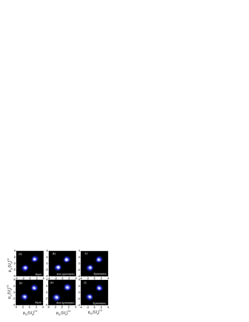
Figure 1: Angle-integrated electron momentum distributions as functions of the momentum components $(p_{1\parallel},p_{2\parallel})$ parallel to the laser-field polarization, computed using the contact-type interaction (25). The field intensity and frequency have been taken as $I=1.5\times 10^{14}\mathrm{W/cm}^{2}$, and $\omega=0.057$ a.u., respectively, and the ionization potentials $E_{01}=0.573$ a.u. and $E_{02}=0.997$ a.u.correspond to $N_{2}$ at the equilibrium internuclear distance $R=2.068$ a.u. The upper and lower panels have been calculated in the velocity and the length gauge, respectively. Panels (a), and (d) correspond to the single atom case, panels (b) and (e) to the symmetric prefactors (8) and (11), and panels (c) and (f) to the antisymmetric prefactors (9) and (12).

Figure 1 depicts the above-mentioned distributions. In general, even though different gauges and orbital symmetry lead to very distinct prefactors, the shapes of the distributions are very similar. This is due to the fact that the momentum region for which the transition amplitude (1) has a classical counterpart is relatively small. Indeed, we have verified that, for vanishing transverse momenta $p_{1\perp}=$ $p_{2\perp}=0$, this region starts slightly below $\pm\sqrt{U_{p}},$ and extends to almost $\pm 3\sqrt{U_{p}}.$ This is the case for which the classically allowed region is the most extensive, so that below $\pm\sqrt{U_{p}}$ the contributions to the yield are negligible. Hence, the maxima and the shapes of these distributions are determined by the interplay between phase-space effects and the prefactor (26).

In the length gauge, Eq. (26) is very large near $p_{1\parallel}+$ $p_{2\parallel}=\pm 1.5\sqrt{U_{p}},$ while in the velocity gauge this holds for $p_{1\parallel}+$ $p_{2\parallel}=\pm 0.5\sqrt{U_{p}}$. This is in agreement with the features displayed in Fig. 1. In fact, a closer inspection of the length-gauge distributions shows that they exhibit slightly larger maxima, near $p_{1\parallel}=p_{2\parallel}=\pm 1.5\sqrt{U_{p}}$, and are broader along $p_{1\parallel}=-p_{2\parallel}$ than their velocity-gauge counterparts. In the velocity gauge, since the peak of the prefactor lies outside the classically allowed region, we expect that the yield will be maximal near the smallest momentum values which have a classical counterpart. This agrees with Figs. 1(a)-(c), which exhibit peaks slightly above $\pm\sqrt{U_{p}}$.

In Fig. 1, one also notices that the distributions are nearly identical in the single-atom and molecular case. This is possibly due to the fact that the distributions are being angle-integrated. Apart from that, we have verified that, within the classically allowed region, there is at most a single interference minimum. This may additionally contribute for the lack of well-defined interference patterns.

III.2 Interference effects

For the above-stated reasons, in order to investigate whether interference patterns are present in the NSDI electron momentum distributions, we will proceed in many ways. First, we will increase the classically allowed momentum region, and hence the radius of the hypersphere given by Eq. (19). For that purpose, we will increase the intensity of the driving laser field. Second, in this section, we will consider aligned molecules, as it is not clear whether integrating over the alignment angle washes the interference patterns out. One should note that, for the parameters considered in this work, the De Broglie wavelength of the returning electron is much larger than the equilibrium internuclear distance of $N_{2}$.

Finally, in order to disentangle the influence of the prefactor which accounts for the two-center interference from that of $\varphi_{0}^{(2)}(\mathbf{\mathcal{P}}(t)),$ we make the further assumption that $V_{12}$ is placed at the position of the ions. Without this assumption, prefactor (26) corresponding to the contact interaction depends on the final electron momenta, and thus introduces a bias in the distributions. This may obscure any effects caused solely by the molecular prefactors.

Explicitly, this reads

$$V_{12}=\delta(\mathbf{r}_{1}-\mathbf{r}_{2})\left[\delta(\mathbf{r}_{2}-\mathbf{R}/2)+\delta(\mathbf{r}_{2}+\mathbf{R}/2)\right].$$ (27)

Such an interaction has been successfully employed in the single-atom case, and led to “balloon-shaped” distributions peaked near $p_{1\parallel}=p_{2\parallel}=\pm 2\sqrt{U_{p}}.$ Such distributions exhibited a reasonable degree of agreement with the experiments FSLB2004 . This choice of $V_{12}$ yields $\varphi_{0}^{(2)}(\mathbf{\mathcal{P}}(t))=const$, in addition to $V_{12}(\mathbf{p}_{1}-\mathbf{k})=const.$ Hence, apart from effects caused by the integration over momentum space, the shape of the distributions will be mainly determined by the cosine or sine factor in Eqs. (11) or (12). The former and the latter case correspond to the symmetric or antisymmetric case, respectively. The explicit interference maxima and minima are given by Eq. (15).

We will now perform a more detailed analysis of such interference condition. In terms of the momentum components $p_{i\parallel},$ or $p_{i\perp}$ $(i=1,2),$ parallel or perpendicular to the laser-field polarization, this condition may be written as $\cos\left[\zeta R/2\right]$ or $\sin\left[\zeta R/2\right],$ in terms of the argument $\zeta.$ Explicitly, this argument is given by

$$\zeta=\zeta_{\parallel}+\zeta_{\perp},$$ (28)

with

$$\zeta_{\parallel}=\left[\sum\limits_{i=1}^{2}p_{i\parallel}-k(t)\right]\cos\theta$$ (29)

and

$$\zeta_{\perp}=p_{1\perp}\sin\theta\cos\varphi+p_{2\perp}\sin\theta\cos(\varphi+\alpha).$$ (30)

In the above-stated equations, $\theta$ gives the alignment angle of the molecule, $\varphi$ corresponds to the angle between the perpendicular momentum $\mathbf{p}_{1\perp}$ and the polarization plane, and $\alpha$ yields the angle between both perpendicular momentum components. Since we are dealing with non-resolved transverse momenta, we integrate over the latter two angles. In the velocity and in the length gauge, $k(t)=k$ and $k(t)=k-A(t)$, respectively. Interference extrema will then be given by the condition

$$(\zeta_{\perp}+\zeta_{\parallel})R=n\pi.$$ (31)

For a symmetric linear combination of atomic orbitals, even and odd $n$ correspond to interference maxima and minima, respectively, whereas, in the antisymmetric case, this condition is reversed.

An inspection of Eqs. (29) and (30), together with the above-stated condition, provides an intuitive picture of how the interference patterns change with the alignment angle $\theta.$ For parallel alignment, the only contributions to such patterns will be due to $\zeta_{\parallel}$. In this particular case, the interference condition may be written as

$$p_{1\parallel}+p_{2\parallel}=\frac{n\pi}{R\cos\theta}+k(t),$$ (32)

where $\cos\theta=1$. Eq. (32) implies the existence of well-defined interference maxima or minima, which, to first approximation, are parallel to the anti-diagonal $p_{1\parallel}=-p_{2\parallel}.$ This is only an approximate picture, as $k$, according to the saddle-point equation (17), is dependent on the start time $t^{\prime}$ and on the return time $t$. Furthermore, since $t^{\prime}$ and $t$ also depend on the transverse momenta of the electrons (see FB2003 for a more detailed discussion), Eq. (32) is influenced by such momenta. Finally, in the length gauge, there is an additional time dependence via the vector potential $\mathbf{A}(t)$ at the instant of rescattering.

As the alignment angle increases, the contributions from the term $\mathbf{\zeta}_{\perp}$ related to the transverse momenta start to play an increasingly important role in determining the interference conditions. The main effect such contributions have is to weaken the fringes defined by Eq. (32), until, for perpendicular alignment, the fringes completely vanish and the electron momentum distributions resemble those obtained for a single atom. This can be readily seen if we consider the interference condition for $\theta=\pi/2$, which is

$$p_{1\perp}\cos\varphi+p_{2\perp}\cos(\varphi+\alpha)=\frac{n\pi}{R}.$$ (33)

Eq. (33) gives interference conditions which do not depend on $k(t)$, and which vary with the angles $\varphi$ and $\alpha.$ As one integrates over the latter parameters, which is the procedure adopted for distributions with non-resolved transverse momentum, any structure which may exist in Eq. (33) is washed out.

In Fig. 2, we display electron momentum distributions computed in the velocity gauge for a symmetric highest occupied molecular orbital and various alignment angles. The symmetric case is of particular interest, since, recently, NSDI electron momentum distributions have been measured for aligned $N_{2}$ molecules NSDIalign . For parallel alignment, interference fringes parallel to the anti-diagonal $p_{1\parallel}=-p_{2\parallel}$ can be clearly seen, according to Eq. (32). For small alignment angles, such as that in Fig. 2(b), the maxima and minima start to move towards larger parallel momenta. Furthermore, there exists an increase in the momentum difference between consecutive maxima or minima, and the interference fringes become less defined. This is due to the fact that the term $\mathbf{\zeta}_{\perp}$, which washes out the interference patterns, is getting increasingly prominent. For large alignment angles, such as that in Fig. 2(c), the contributions from this term are very prominent and have practically washed out the two-center interference. Finally, for perpendicular alignment, the distributions resemble very much those obtained for the single-atom case, i.e., circular distributions peaked at $p_{1\parallel}=p_{2\parallel}=\pm 2\sqrt{U_{p}}$ (c.f. Refs. FSLB2004 ; FL2005 for details). This is expected, since the term responsible for the two-center interference fringes is vanishing for $\theta=90^{0}$.

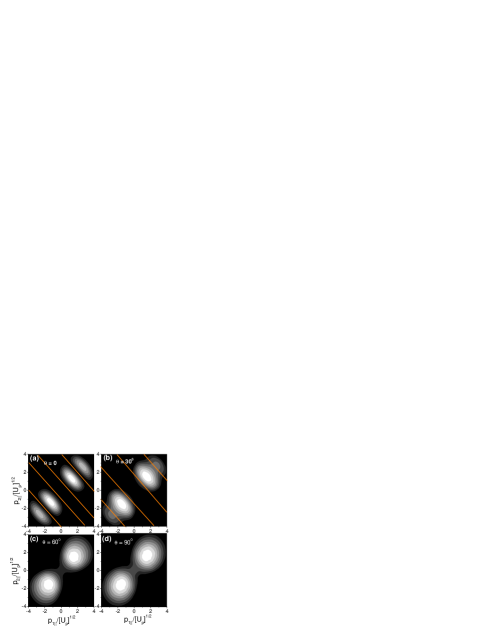
Figure 2: Electron momentum distributions as functions of the parallel momenta $(p_{1\parallel},p_{2\parallel})$, for several alignment angles. We consider the velocity gauge, symmetric orbitals, and driving-field intensity $I=5\times 10^{14}\mathrm{W/cm}^{2}$. The remaining field and molecular parameters are the same as in the previous figure. The position of the interference minima, estimated by assuming that the first electron returns at a field crossing, are indicated by the lines in the figure. Panel (a), (b), (c) and (d) correspond to alignment angles $\theta=0,\theta=30^{0},$ $\theta=60^{0}$ and $\theta=90^{0},$ respectively.

The fringes in Fig. 2 exhibit a very good qualitative agreement with the interference conditions derived in this section. Furthermore, the figure shows that, for some alignment angles, the patterns caused by the two-center interference survive the integration over the transverse momentum components. It is not clear, however, how well the position of the fringes agree with Eq. (32) quantitatively, and if it is possible to provide simple estimates for these maxima and minima. Apart from that, it is not an obvious fact that the patterns survive the integration over the transverse momentum, and one should understand why this happens.

In particular, the role of the intermediate momentum of the first electron will be analyzed subsequently. According to the return condition (17), this quantity depends on the start and return times of the first electron. Furthermore, in the length gauge, the interference condition also depends on the vector potential $A(t_{1})$ at the return time of the first electron. For each pair $(p_{1\parallel},p_{2\parallel})$, the emission and return times are strongly dependent on the transverse momenta FB2003 . Apart from that, physically, there are several orbits along which the first electron may return, which occur in pairs. Hence, there exist several possible values for $k$. In practice, only the two shortest orbits contribute significantly to the yield. The contributions from the remaining pairs are strongly suppressed due to wave-packet spreading. However, this still means that the intermediate momentum, and therefore the position of the maxima and minima, has two possible values, which depend on the start and return times, and also on the final momentum components.

We have made a rough estimate of the position of these patterns for parallel alignment, in the velocity and length gauges, along the diagonal $p_{1\parallel}=p_{2\parallel}=p_{\parallel}$. This estimate is given in Table 1. For symmetric highest occupied molecular orbitals, the even and odd numbers denote maxima and minima, respectively, while for antisymmetric orbits this role is reversed. Thereby, we assumed that the first electron left at peak field and returned at a field crossing. This gives $|k|\simeq\sqrt{U_{p}}/(0.75\pi)$ in the saddle-point equation (17). Furthermore, in the length-gauge estimate, we took $|A(t)|\simeq 2\sqrt{U_{p}}$. We have verified that both quantities are negative for the orbits in question.

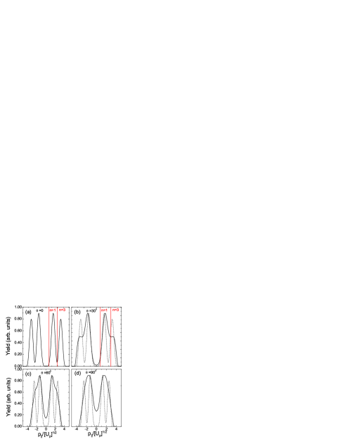
Figure 3: Electron momentum distributions for parallel momenta $p_{1\parallel}=p_{2\parallel}=p_{\parallel},$ non-resolved transverse momenta and several alignment angles. We consider the velocity gauge, symmetric orbitals, and the same molecule and field parameters as in the previous figure. The position of the interference minima, estimated by assuming that the first electron returns at a field crossing, are indicated by the vertical lines in the figure. Panel (a), (b), (c) and (d) correspond to alignment angles $\theta=0,\theta=30^{0},$ $\theta=60^{0}$ and $\theta=90^{0},$ respectively. For comparison, the yield for $\theta=0$ are indicated as the dashed lines in the figure. To facilitate the comparison, the yields have been normalized to the same peak values.

These estimates agree reasonably well with the electron momentum distributions along $p_{1\parallel}=p_{2\parallel}=p_{\parallel}$. These distributions are depicted in Fig. 3 for several alignment angles, the velocity gauge, and symmetric highest occupied molecular orbitals. The positions of the minima, for each angle, are indicated in the figure. These minima have been computed employing Eq. (32) and the above-stated estimate for $k$. For parallel alignment [Fig. 3(a)], the position of the extrema agree relatively well with Table 1. This suggests that the intermediate momentum of the first electron, upon return, can be approximated by its value at the field crossing. As the alignment angle increases, the patterns become increasingly blurred until they are eventually washed out by the contributions of $\zeta_{\perp}$. For instance, for $\theta=30^{0}$ [Fig. 3(b)], one may still identify a change of slope in the distributions, at the momentum for which the minima $n=3$ is expected to occur. For $\theta=60^{0},$ however, the term $\zeta_{\perp}$ has already washed out the interference patterns. Indeed, in Fig. 3(c), there is no evidence of interference patterns. Finally, for perpendicular alignment, the distributions resemble very much those obtained in the single-atom case, as shown in [Fig. 3(d)].

Extrema	Parallel momentum $p_{\parallel}/[U_{p}]^{1/2}$
Order $n$	velocity gauge  length gauge
1	0.513                       1.513
2	1.239                       2.239
3	1.964                       2.964
4	2.689                       3.689

Table 1: Electron momenta corresponding to the interference maxima and minima given by Eq. (26), in the velocity and length gauges, for a parallel-aligned molecule, for the same field and molecule parameters as in Fig. 3. The parallel momenta $p_{\parallel}$ have been taken to be along the diagonal $p_{1\parallel}=p_{2\parallel}$ in the momentum plane, and the transverse momenta are assumed to be vanishing. If the highest occupied molecular orbital is approximated by a symmetric combination of atomic orbitals, the maxima and minima are denoted by even and odd number, while in the antisymmetric case, this role is reversed, i.e., odd and even numbers denote maxima and minima, respectively.

In order to investigate the behavior of the intermediate momentum $k$ with respect to $p_{n\perp}(n=1,2)$, we will compute electron momentum distributions keeping the absolute values of the transverse momenta fixed. For simplicity, we will take $\theta=0$ and parallel momenta along the diagonal, i.e., $p_{1\parallel}=p_{2\parallel}=p_{\parallel}$. These distributions are displayed in Fig. 4. In this case, there exists a region of parallel momenta for which the yield is oscillating, between a maximum and a minimum parallel momentum. These oscillations are due to the quantum interference between the two shortest possible orbits along which the first electron may return. These orbits constitute the pair that has been employed in the computations performed in this work. The larger the transverse momenta are, the less extensive this region is. This is expected according to Eq. (19), which delimits this region (for details see Ref. FB2003 ).

Apart from these oscillations, Fig. 4 also exhibits the maxima and minima caused by the spatial two-center interference. The figure shows that the position of such patterns is very robust with respect to the choice of $p_{\perp n}$, $n=1,2$. Indeed, both maxima and minima remain at practically the same positions, if different transverse momenta are taken. For this reason, such patterns survive if one integrates over the transverse momenta. In contrast, the oscillations due to the temporal interference get washed out. For the parameters employed in the figure, we have verified a reasonable agreement between the second minimum and Table 1. The first minimum is to a large extent washed out by the contributions of the events displaced by a half-cycle, i.e., which are related to the transition amplitude $M_{L}$.

Interference fringes parallel to $p_{1\parallel}=-p_{2\parallel}$ are also present in the length gauge, and for antisymmetric orbitals. This is shown in the upper panels of Fig. 5, for parallel alignment angle. In fact, the main difference as compared to the symmetric, velocity-gauge case, is the position of such patterns, in agreement with Eq. (32). There is also some blurring in the patterns, in the length gauge, possibly caused by the fact that the vector potential $\mathbf{A}(t)$ depends on the return time $t.$ This latter quantity is different for different transverse momenta. The patterns, however, can be also clearly identified in this gauge. In all cases, however, there is no evidence of a straightforward connection between an enhancement or suppression of the yield in the low-momentum region and the symmetry of the orbital. For instance, in the velocity gauge, the yield is enhanced if the orbital is antisymmetric. The length-gauge distributions, on the other hand, exhibit a suppression in that region regardless of the orbital symmetry.

In the lower panels of Fig. 5, we display the distributions along  $p_{1\parallel}=p_{2\parallel}=p_{\parallel}$. Similarly to the velocity-gauge, symmetric case, the minima and maxima of the distributions roughly agree with Table 1. In fact, the even numbers in this table roughly give the position of the minima in Figs. 5(e) and (f), which correspond to antisymmetric orbitals, while the odd numbers approximately yield the minima in Fig. 5(d), which display the length-gauge, symmetric case. Specifically for the length-gauge distributions [Figs. 5(d) and (e)], there is an overall displacement of roughly $2\sqrt{U_{p}}$ in the position of the patterns. This is consistent with the modified interference conditions in this case.

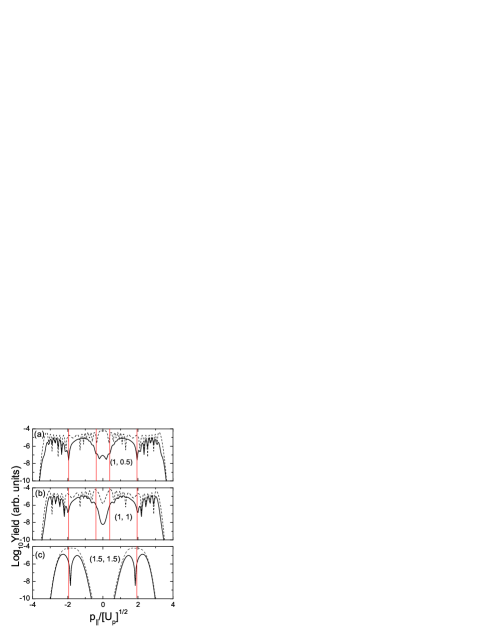
Figure 4: Electron momentum distributions for resolved transverse momenta, as functions of the parallel momentum $p_{1\parallel}=p_{2\parallel}=p_{\parallel},$ for alignment angle $\theta=0$. We consider the velocity gauge, symmetric orbitals, and the same molecule and field parameters as in the previous figure. For comparison, the corresponding single-atom distributions are presented as the dashed lines in the figure. The interference minima according to Table 1 are indicated by the vertical lines in the figure. The numbers in the figure indicate the transverse momentum components $(p_{1\perp},$ $p_{2\perp})$ in units of $\sqrt{U_{p}}.$

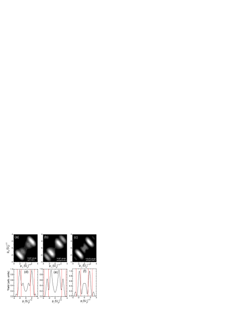
Figure 5: Electron momentum distributions for a parallel-aligned molecule ($\theta=0$), different orbital symmetries and gauges. The upper and lower panels give the contour plots as functions of the parallel momenta, and the distributions along $p_{1\parallel}=p_{2\parallel}=p_{\parallel},$ respectively. We integrate over the transverse momenta, and employ the same molecule and field parameters as in the previous figures. The interference minima according to Table 1 are indicated by the vertical lines in the figure. Panel (a) and (d), (b) and (e), and (c) and (f) correspond to symmetric orbitals in the length gauge, antisymmetric orbitals in the length gauge and antisymmetric orbitals in the velocity gauge, respectively. For panels (d), (e) and (f), the units in the vertical axis have been chosen so that their upper values are unity (the original values have been divided by 0.016, 0.01 and 0.04, respectively).

III.3 The classical limit

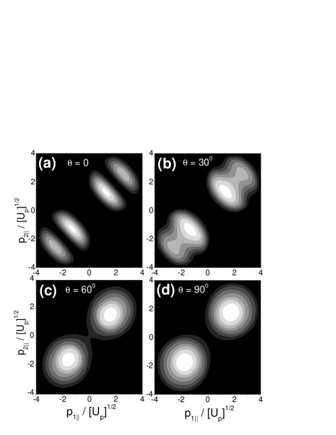
Figure 6: Electron momentum distributions for symmetric highest occupied molecular orbitals and several alignment angles, as functions of the parallel momentum components $(p_{1\parallel}$, $p_{2\parallel})$, computed in the velocity gauge using the classical model for the same field and molecular parameters as in Fig. 2. Panels (a), (b), (c) and (d) correspond to $\theta=0$, $\theta=30^{0}$, $\theta=60^{0}$, and $\theta=90^{0}$, respectively.

In the following, we perform a comparison between the S-Matrix computation and its classical limit. In the single-atom case, both computations led to very similar results, unless the driving-field intensity is close to the threshold intensity thresh2006 . At this intensity, the kinetic energy upon return is just enough to make the second electron overcome the ionization potential. Therefore, since the intensity used in most figures is far above the threshold intensity, one would expect similar results.

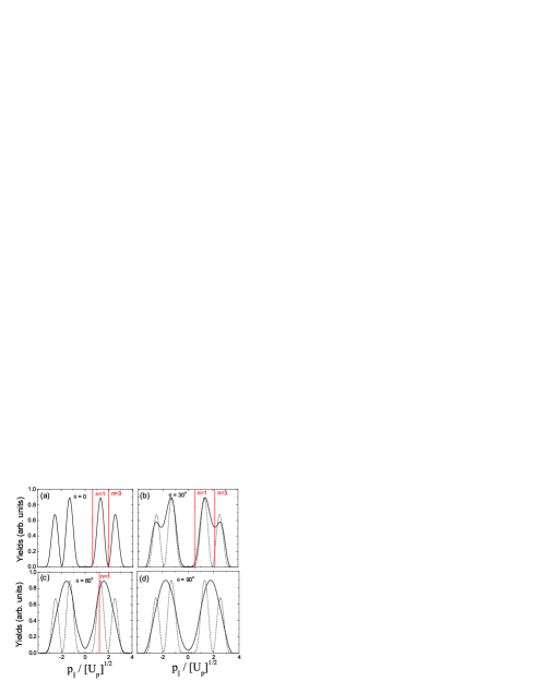
Figure 7: Electron momentum distributions for symmetric highest occupied molecular orbitals and several alignment angles, along $p_{1\parallel}=p_{2\parallel}=p_{\parallel}$, computed in the velocity gauge using the classical model for the same field and molecular parameters as in Fig. 3. Panels (a), (b), (c) and (d) correspond to $\theta=0$, $\theta=30^{0}$, $\theta=60^{0}$, and $\theta=90^{0}$, respectively.

In Fig. 6, we display differential momentum distributions as functions of the parallel momentum components, computed employing the classical model. This is the classical counterpart of Fig. 2, in which the quantum mechanical distributions are depicted for the same parameters. Indeed, for all alignment angles depicted, the classical and quantum-mechanical distributions look very similar. Hence, even though the two-center interference is an intrinsically quantum mechanical effect, it can be mimicked to a very large extent within a classical model. There is also a good quantitative agreement between the positions of the minima and maxima in both classical and quantum mechanical cases. This is shown in Fig. 7, for parallel momenta $p_{1\parallel}=p_{2\parallel}=p_{\parallel}$, and several alignment angles. For $\theta=0$ and $\theta=30^{0}$ [Figs. 7(a) and 7(b), respectively], the maxima and minima agree very well with those in Fig. 3. The main difference, with regard to the quantum-mechanical case, is that, for large alignment angles, the classical distributions are more localized than their quantum-mechanical counterparts, especially in the low momentum regions. For instance, in Fig. 7(d), the yield is much lower near $p_{\parallel}=0$, as compared to the outcome of the S-Matrix computation [Fig. 3(d)]. This discrepancy is possibly due to the fact that the classical model underestimates contributions to the yield near the boundary of the classically allowed region.

IV Conclusions

In this work, we addressed two aspects of non-sequential double ionization of diatomic molecules: the influence of the symmetry of the highest occupied molecular orbital, and of the alignment angle, on the differential electron momentum distributions. We considered the physical mechanism of electron-impact ionization, within the strong-field approximation, and very simple models for the highest occupied molecular orbitals, within the LCAO and frozen nuclei approximations.

For angle-integrated electron momentum distributions, we have shown that, for driving-field intensities within the tunneling regime and compatible with existing experiments NSDIsymm , the distributions computed with symmetric and antisymmetric orbitals (prefactors (11) and (12), respectively), or different gauges, look practically identical. This is due to the fact that, if only electron-impact ionization is taken into account, the momentum region for which this process has a classical counterpart is too small to allow the corresponding pre-factors to have a significant influence. At first sight, this is in contradiction with the experimental findings and computations in NSDIsymm . Therein, a broadening parallel the anti-diagonal direction has been reported only for the anti-symmetric case, while, for a symmetric combination of atomic orbitals, an elongation in the direction $p_{1\parallel}=p_{2\parallel}$ has been observed. One should note, however, that, in NSDIsymm , an effective, time-dependent second ionization potential $\ E_{02}(t)=E_{02}-2\sqrt{2|E(t)|}$ is used Threshold . This feature has not been incorporated in the present computations. It has the effect of increasing the classically allowed momentum region and introducing an additional time dependence in the prefactors and the action.

We have also made a detailed assessment of the interference effects due to the fact that electron emission may occur from two spatially separated centers. In order to disentangle the interference effects from those caused by the prefactor $\varphi_{0}^{(2)}(\mathbf{\mathcal{P}}(t))$, we assumed that the second electron was dislodged by a contact-type interaction at the position of the ions. We have observed interference fringes in the electron momentum distributions, along $p_{1\parallel}=-p_{2\parallel}+const$ for all gauges and orbital symmetries. These fringes are most pronounced if the molecule is aligned parallel to the laser-field polarization. As the alignment angle increases, it gets washed out by the term (33), which, for angle-integrated momenta, is essentially isotropic in the perpendicular momentum plane. Consequently, the peaks of the distributions shift towards higher momenta, and their shapes resemble more and more those obtained for the same type of interaction in the single-atom case. We have also found that the prominence of such peaks will depend on the integration over the electron transverse momenta, so that some maxima may be more prominent than others.

Interestingly, we are able to observe changes in the peak momenta of the distributions, as the alignment is varied, even if a single physical mechanism, namely electron-impact ionization, is considered. These changes are caused by the two-center interference effects. This complements recent results, in which different types of collisions and double-ionization mechanisms are associated with changes in the peaks of NSDI distributions, within the context of molecules NSDIalign ; Beijing2007 . Finally, for laser-field intensities within the tunneling regime, the distributions obtained including only electron-impact ionization are far more localized than those reported experimentally, and the differences between different gauges and orbital symmetries are barely noticeable. In order to assess such effects, it was necessary to consider much higher intensities, for which other physical mechanisms, such as multiple electron recollisions, would also be expected to play a role Beijing2007 . These discrepancies may be due to the fact that we are not including the physical mechanism in which the first electron, upon return, promotes the second electron to an excited state, from which it subsequently tunnels out.

Acknowledgements: W.Y. would like to thank the University College London for its kind hospitality. This work has been financed by the UK EPSRC (Grant no. EP/D07309X/1) and by the Faculty Research Fund of the School of Mathematics and Physical Sciences (UCL). We also thank the UK EPSRC for the provision of a DTA studentship.

References

- (1) P. B. Corkum, Phys. Rev. Lett. 71, 1994 (1993); K. C. Kulander, K. J. Schafer, and J. L. Krause in: B. Piraux et al. eds., Proceedings of the SILAP conference, (Plenum, New York, 1993).
- (2) A. Scrinzi, M. Y. Ivanov, R. Kienberger, and D. M. Villeneuve, J. Phys. B 39, R1 (2006).
- (3) J. Itatani, J. Levesque, D. Zeidler, H. Niikura, H. Pépin, J. C. Kieffer, P. B. Corkum and D. M. Villeneuve, Nature 432, 867 (2004).
- (4) H. Niikura, F. Légaré, R. Hasbani, A. D. Bandrauk, M. Yu. Ivanov, D. M. Villeneuve and P. B. Corkum, Nature 417, 917 (2002); H. Niikura, F. Légaré, R. Hasbani, M. Yu. Ivanov, D. M. Villeneuve and P. B. Corkum, Nature 421, 826 (2003); S. Baker, J. S. Robinson, C. A. Haworth, H. Teng, R. A. Smith, C. C. Chirilă, M. Lein, J. W. G. Tisch, J. P. Marangos, Science 312, 424 (2006).
- (5) R. Kopold, W. Becker and M. Kleber, Phys. Rev. A 58, 4022 (1998).
- (6) J. Muth-Böhm, A. Becker, and F. H. M. Faisal, Phys. Rev. Lett. 85, 2280 (2000); A. Jarón-Becker, A. Becker, and F. H. M. Faisal, Phys. Rev. A 69, 023410 (2004); A. Requate, A. Becker and F. H. M. Faisal, Phys. Rev. A 73, 033406 (2006).
- (7) T. K. Kjeldsen and L. B. Madsen, J. Phys. B 37, 2033 (2004); Phys. Rev. A 71, 023411 (2005); Phys. Rev. Lett. 95, 073004 (2005); T. K. Kjeldsen, C. Z. Bisgaard, L. B. Madsen, H. Stapelfeld, Phys. Rev. A 71, 013418 (2005); C. B. Madsen and L. B. Madsen, Phys. Rev. A 74, 023403 (2006).
- (8) V. I. Usachenko, and S. I. Chu, Phys. Rev. A 71, 063410 (2005).
- (9) H. Hetzheim, M. Sc. thesis (Humboldt University Berlin, 2005).
- (10) V. I. Usachenko, P. E. Pyak, and Shih-I Chu, Laser Phys. 16, 1326 (2006).
- (11) C. C. Chirilă and M. Lein, Phys. Rev. A 73, 023410 (2006).
- (12) M. Lein, Phys. Rev. Lett. 94, 053004 (2005); C. C. Chirilă and M. Lein, J. Phys. B 39, S437 (2006).
- (13) H. Hetzheim, C. Figueira de Morisson Faria, and W. Becker, Phys. Rev. A 76, 023418 (2007).
- (14) C. Figueira de Morisson Faria, Phys. Rev. A 76, 043407 (2007).
- (15) S. X. Hu and L. A. Collins, Phys. Rev. Lett. 94, 073004 (2005); D. A. Telnov and Shih-I Chu, Phys. Rev. A 71, 013408 (2005).
- (16) G. Lagmago Kamta and A. D. Bandrauk, Phys. Rev. A 70, 011404 (2004); ibid. 71, 053407 (2005).
- (17) X. Zhou, X. M. Tong, Z. X. Zhao and C. D. Lin, Phys. Rev. A 71, 061801(R) (2005); ibid. 72, 033412 (2005).
- (18) D. B. Milošević, Phys. Rev. A 74, 063404 (2006).
- (19) M. Lein, N. Hay, R. Velotta, J. P. Marangos, and P. L. Knight, Phys. Rev. Lett. 88, 183903 (2002); Phys. Rev. A 66, 023805 (2002); M. Spanner, O. Smirnova, P. B. Corkum and M. Y. Ivanov, J. Phys. B 37, L243 (2004).
- (20) X. Liu, C. Figueira de Morisson Faria, W. Becker and P.B. Corkum, J. Phys. B. 39, L305 (2006)
- (21) C. Cornaggia and Ph. Hering, J. Phys. B 31, L503-L510 (1998).
- (22) E. Eremina, X. Liu, H. Rottke, W. Sandner, M.G. Schätzel, A. Dreischuch, G.G. Paulus, H. Walther, R. Moshammer and J. Ullrich, Phys. Rev. Lett. 92, 173001 (2004).
- (23) D. Zeidler, A. Staudte, A. B. Bardon, D. M. Villeneuve, R. Dörner, and P. B. Corkum, Phys. Rev. Lett. 95, 203003 (2005).
- (24) For a review on this subject see, e.g., R. Dörner, Th. Weber, M. Weckenbrock, A. Staudte, M. Hattas, H. Schmidt-Böcking, R. Moshammer, J. Ullrich: Adv. At., Mol., Opt. Phys. 48, 1 (2002).
- (25) S. Baier, C. Ruiz, L. Plaja, and A. Becker, Phys. Rev. A 74, 033405 (2006); Laser Phys. 17, 358 (2007).
- (26) C. Figueira de Morisson Faria, H. Schomerus, X. Liu, and W. Becker, Phys. Rev. A 69, 043405 (2004).
- (27) C. Figueira de Morisson Faria, and M. Lewenstein, J. Phys. B 38, 3251 (2005).
- (28) R. Santra and A. Gordon, Phys. Rev. Lett. 96, 073906 (2006); A. Gordon, F. X. Kärtner, N. Rohringer and R. Santra, Phys. Rev. Lett. 96, 223902 (2006); S. Patchkovskii, Z. Zhao, T. Brabec and D. Villeneuve, J. Chem. Phys. 126, 114306 (2007).
- (29) O. Smirnova, M. Spanner and M. Ivanov, J. Phys. B 39, S307 (2006); O. Smirnova, M. Spanner and M. Ivanov, J. Mod. Opt. 54, 1019 (2007).
- (30) W. Becker, J. Chen, S. G. Chen, and D. B. Milošević, Phys. Rev. A 76, 033403 (2007).
- (31) P. Salières, B. Carré, L. LeDéroff, F. Grasbon, G. G. Paulus, H. Walther, R. Kopold, W. Becker, D. B. Milošević, A. Sanpera and M. Lewenstein, Science 292, 902 (2001).
- (32) X. Liu and C. Figueira de Morisson Faria, Phys. Rev. Lett. 92, 133006 (2004); C. Figueira de Morisson Faria, X. Liu, A. Sanpera and M. Lewenstein, Phys. Rev. A 70, 043406 (2004)
- (33) C. Figueira de Morisson Faria, H. Schomerus and W. Becker, Phys. Rev. A 66, 043413 (2002).
- (34) C. Figueira de Morisson Faria and W. Becker, Laser Phys. 13, 1196 (2003).
- (35) C. Figueira de Morisson Faria, X. Liu and W.Becker, J. Mod. Opt. 53, 193 (2006).
- (36) E. Eremina, X. Liu, H. Rottke, W. Sandner, A. Dreischuch, F. Lindner, F. Grasbon, G.G. Paulus, H. Walther, R. Moshammer, B. Feuerstein, and J. Ullrich, J. Phys. B. 36, 3269 (2003).
- (37) J. Liu, D.F. Ye, J. Chen, and X. Liu, Phys. Rev. Lett. 99, 013003 (2007).