Dissipation and entanglement dynamics for two interacting qubits coupled to independent reservoirs

Abstract

We derive the master equation of a system of two coupled qubits by taking into account their interaction with two independent bosonic baths. Important features of the dynamics are brought to light, such as the structure of the stationary state at general temperatures and the behaviour of the entanglement at zero temperature, showing the phenomena of sudden death and sudden birth as well as the presence of stationary entanglement for long times. The model here presented is quite versatile and can be of interest in the study of both Josephson junction architectures and cavity-QED.

1 Introduction

During the last two decades the problem of controlling the coherent time evolution of quantum systems has received a great deal of attention both because it could lead to a deeper understanding of fundamental aspects of quantum mechanics and because it is of interest for applications [1]. The possibility of generating and controlling non classical correlations (i.e. entangled states) in multipartite systems, despite their coupling with an external environment, is a fundamental ingredient for instance in the theory of quantum measurement and in the study of the border between the quantum world and the macroscopic classical world [2]. In addition such a possibility is an essential goal in the field of quantum computing and quantum information theory [3]. It is well known that the interaction of an open quantum system with an external reservoir is an important source of dissipation and decoherence. In order to describe such phenomena, a master equation approach can be used [4, 5, 6]. In particular, following Ref. [6], one has at his disposal a general formalism allowing to derive the quantum master equation of a general quantum system, provided one knows the Hamiltonian governing the unitary part of its dynamics. Exploiting this recipe, one can see that the dissipative dynamics, in the Born-Markov and rotating wave approximations, is described by a master equation in which the quantum jumps occur among eigenstates of the Hamiltonian of the open quantum system under scrutiny. This microscopic approach may be sometimes in contrast with some phenomenological approaches to quantum dissipative dynamics present in the literature, as one can see for example in Refs. [7, 8, 9].

Within this framework and with the aforementioned approach, here we analyze the dynamical behavior of the entanglement between two coupled two-state systems each of them interacting with a bosonic bath. The model is quite versatile and can be exploited, for instance, in order to describe the dipole-dipole (flux or charge) interaction of two distant atomic (flux or charge) qubits. In the case of Josephson flux qubits the coupling term corresponds to a flux-flux coupling proportional to their mutual inductance [10]. It is worth noting that the same model can be used to describe richer physical situations, for instance the coupling between a Josephson junction based qubit in the charge regime with an impurity located in the substrate of the device [13]. In this case the qubit can be thought as coupled with external environmental degrees of freedom describing the auxiliary circuitry (necessary, for instance, for the qubit control and the redout) which can be modeled as an infinite bath of harmonic oscillators, while the substrate impurity may interact with a phononic bath.

Starting from such a model of qubit-qubit interaction, and including counter-rotating terms in the system Hamiltonian, we derive a quantum master equation in order to describe the dissipative dynamics of the two-qubit system, concentrating on some aspects such as the structure of the stationary state of the system and the time evolution of the entanglement between the two qubits. The entanglement dynamics of open bipartite quantum systems has been studied in previous works, for example in Refs. [11, 12, 14], bringing to light important features such as the complete disentanglement of the system in a finite time (entanglement sudden death), and, in the case of Ref. [14], the sudden reappearance of entanglement (sudden birth). In the latter case, the presence of stationary entanglement for very long times has been related to the presence of a reservoir common to the two subsystems, so that the non-local correlations between them can be thought of as due to the mediation of the environment. In this paper we will show that stationary entanglement can occur also in the case wherein the two qubits interact with two independent reservoirs, provided the interaction between the two subsystems contains also counter-rotating terms, which are usually neglected in the literature. In such a case, the stationary entanglement occurs because the counter-rotating terms cause the ground state of the system to be an entangled state of the bipartite system.

The paper is structured as follows. In section 2 we introduce the model previously described and we microscopically derive the Markovian master equation in the weak damping limit assuming that the two reservoir are independent and with arbitrary temperatures, $T_{1}$ and $T_{2}$. Therefore, in section 4, we analyze the dynamics of the system in the limit case $T_{1}=T_{2}=0$ discussing the stationary entanglement and the features of its time evolution considering different initial conditions for the bipartite system. Finally, conclusive remarks are given in section 5.

2 The model

Let us consider two interacting two-level systems and let us call $|{0}\rangle_{1}$ ($|{0}\rangle_{2}$) the ground state of the first (second) system and $|{1}\rangle_{1}$ ($|{1}\rangle_{2}$) the corresponding excited state. Let us assume that the two systems are coupled in such a way that their unitary dynamics is governed by the following Hamiltonian (in units of $\hbar$):

$$H_{S}=\omega_{1}\sigma_{+}^{(1)}\sigma_{-}^{(1)}+\omega_{2}\sigma_{+}^{(2)}\sigma_{-}^{(2)}+\frac{\lambda}{2}\,\sigma_{x}^{(1)}\sigma_{x}^{(2)},$$ (1)

where $\omega_{i}$ is the Bohr frequency of the $i$-th two-level system, $\lambda/2$ is the coupling constant and where we have used the Pauli operators $\sigma_{+}^{(i)}=\left|1\right>{}_{i}{}_{i}\left<0\right|$, $\sigma_{-}^{(i)}=\left|0\right>{}_{i}{}_{i}\left<1\right|$ and $\sigma_{x}^{(i)}=\sigma_{+}^{(i)}+\sigma_{-}^{(i)}$, with $i=1,2$. In the case of Josephson flux qubits the coupling term in Eq. (1) corresponds to a flux-flux coupling with $\lambda/2$ proportional to their mutual inductance [10].

It is worth noting that in the Hamiltonian also the counter-rotating terms of the interaction have been included and we will see that they play a central role in the dynamics of the entanglement between the two systems.

The model in Eq. (1) can be exactly diagonalized. By exploiting the fact that the Hamiltonian $H_{S}$ in the uncoupled basis $\left\{|{00}\rangle,|{11}\rangle,|{10}\rangle,|{01}\rangle\right\}$, where for instance $|{00}\rangle=|{0}\rangle_{1}\otimes|{0}\rangle_{2}$, is block diagonal, it is straightforward to show that the eigenvalues (given for increasing energies) are:

$$E_{a}=\frac{1}{2}\left(\omega_{1}+\omega_{2}\right)-\frac{1}{2}\sqrt{\left(\omega_{2}+\omega_{1}\right)^{2}+\lambda^{2}}$$

$$E_{b}=\frac{1}{2}\left(\omega_{1}+\omega_{2}\right)-\frac{1}{2}\sqrt{\left(\omega_{2}-\omega_{1}\right)^{2}+\lambda^{2}}$$

$$E_{c}=\frac{1}{2}\left(\omega_{1}+\omega_{2}\right)+\frac{1}{2}\sqrt{\left(\omega_{2}-\omega_{1}\right)^{2}+\lambda^{2}}$$

$$E_{d}=\frac{1}{2}\left(\omega_{1}+\omega_{2}\right)+\frac{1}{2}\sqrt{\left(\omega_{2}+\omega_{1}\right)^{2}+\lambda^{2}},$$ (2)

while the corresponding eigenstates are:

$$|{a}\rangle=\cos\frac{\theta_{I}}{2}|{00}\rangle-\sin\frac{\theta_{I}}{2}|{11}\rangle$$

$$|{b}\rangle=\cos\frac{\theta_{II}}{2}|{10}\rangle-\sin\frac{\theta_{II}}{2}|{01}\rangle$$

$$|{c}\rangle=\sin\frac{\theta_{II}}{2}|{10}\rangle+\cos\frac{\theta_{II}}{2}|{01}\rangle$$

$$|{d}\rangle=\sin\frac{\theta_{I}}{2}|{00}\rangle+\cos\frac{\theta_{I}}{2}|{11}\rangle.$$ (3)

Here $\omega_{2}\geq\omega_{1}$ and the parameters $\theta_{I}$ and $\theta_{II}$ satisfy the relations:

$$\sin\theta_{I}=\frac{\left|\lambda\right|}{\sqrt{\left(\omega_{2}+\omega_{1}\right)^{2}+\lambda^{2}}},\; \cos\theta_{I}=\frac{\omega_{1}+\omega_{2}}{\sqrt{\left(\omega_{2}+\omega_{1}\right)^{2}+\lambda^{2}}}$$ (4)

$$\sin\theta_{II}=\frac{\left|\lambda\right|}{\sqrt{\left(\omega_{2}-\omega_{1}\right)^{2}+\lambda^{2}}},\; \cos\theta_{II}=\frac{\omega_{2}-\omega_{1}}{\sqrt{\left(\omega_{2}-\omega_{1}\right)^{2}+\lambda^{2}}}$$ (5)

The losses in the system under scrutiny will be taken into account by considering the coupling between the $i$-th system and its own reservoir at temperature $T_{i}$. In the following we will consider the case of independent bosonic reservoirs, whose temperatures, in the general case, can take different values. The total Hamiltonian of the bipartite system and the reservoirs can thus be written as follows:

$$H=H_{S}+H_{E}+H_{\mathrm{int}}$$

$$H_{E}=\sum_{k}\omega_{k}a_{k}^{\dagger}a_{k}+\sum_{j}\omega_{j}b_{j}^{\dagger}b_{j}$$

$$H_{\mathrm{int}}=\sigma_{x}^{(1)}\otimes\sum_{k}\epsilon_{k}\left(a_{k}+a_{k}^{\dagger}\right)+\sigma_{x}^{(2)}\otimes\sum_{j}g_{j}\left(b_{j}+b_{j}^{\dagger}\right).$$ (6)

Here $a_{k}$ ($a_{k}^{\dagger}$) is the annihilation (creation) operator of the $k$-th mode (of frequency $\omega_{k}$) of the reservoir interacting with the first subsystem and similarly $b_{j}$ ($b_{j}^{\dagger}$) is the annihilation (creation) operator of the $j$-th mode (of frequency $\omega_{j}$) of the reservoir interacting with the second subsystem. The parameters $\epsilon_{k}$ and $g_{j}$ are the corresponding coupling constants.

From this model it is possible to microscopically derive the Markovian master equation describing all the relaxation phenomena in the dynamics of the bipartite system under study. To this end in the next section we will exploit the general formalism given in Ref. [6].

3 Derivation of the Markovian master equation in the weak damping limit

From the model in Eq. (2) it is possible to microscopically derive the master equation for the evolution of the bipartite system, by following the general procedure outlined in Ref. [6], in the Born-Markov and rotating wave approximations. The main point of the formalism is that all the jump processes involve transitions between dressed states of the open system under study, i.e. the eigenstates of the Hamiltonian $H_{S}$ of the system, which in our case is given by Eq. (2).

It is well known that, in the Schrödinger picture, the Markovian master equation for a generic open quantum system with Hamiltonian $H_{0}$ is given by [6]:

$$\dot{\rho}(t) = -i\left[H_{0},\rho(t)\right]$$ (7)

$$+ \sum_{\omega}\sum_{\alpha,\beta}\gamma_{\alpha,\beta}(\omega)\left(A_{\beta}(\omega)\rho(t)A_{\alpha}^{\dagger}(\omega)-\frac{1}{2}\left\{A_{\alpha}^{\dagger}(\omega)A_{\beta}(\omega),\rho(t)\right\}\right),$$

where the symbol $\left\{\cdot,\cdot\right\}$ denotes the anticommutator between operators. In the derivation of Eq. (7) we have to assume that the interaction Hamiltonian between the system and the environment is of the form $H_{I}=\sum_{\alpha}A_{\alpha}\otimes B_{\alpha}$, where $A_{\alpha}=A_{\alpha}^{\dagger}$ acts on the Hilbert space of the open system under scrutiny, while $B_{\alpha}=B_{\alpha}^{\dagger}$ acts on the Hilbert space of the environment. In particular, in the case of the model in Eq. (2) the sum consists of two terms, since we have assumed that each two-level system interacts with its own reservoir. In Eq. (7), a renormalization Hamiltonian has been neglected and the rates $\gamma_{\alpha,\beta}(\omega)$ are given by the Fourier transforms of the environment correlation functions, according to:

$$\gamma_{\alpha,\beta}(\omega)=\int_{-\infty}^{+\infty}d\tau\mathrm{e}^{i\omega\tau}\left<B_{\alpha}^{\dagger}(\tau)B_{\beta}(0)\right>.$$ (8)

Concerning the jump operators $A_{\alpha}(\omega)$, their number is given by the number of different Bohr frequencies relative to $H_{0}$ and they can be calculated from the relation [6]:

$$A_{\alpha}(\omega)\equiv\sum_{\epsilon^{\prime}-\epsilon=\omega}\Pi(\epsilon)A_{\alpha}\Pi(\epsilon^{\prime}),$$ (9)

where $\Pi(\epsilon)$ is the projector on the eigenspace of the open system relative to the energy $\epsilon$ and the sum is extended to all the couples of $\epsilon$ and $\epsilon^{\prime}$ such that $\epsilon^{\prime}-\epsilon=\omega$.

For our model we can identify the operators $A_{1}=\sigma_{x}^{(1)}$, $A_{2}=\sigma_{x}^{(2)}$, $B_{1}=\sum_{k}\epsilon_{k}\left(a_{k}+a_{k}^{\dagger}\right)$ and $B_{2}=\sum_{j}g_{j}\left(b_{j}+b_{j}^{\dagger}\right)$. By calculating the matrix elements of $A_{1}$ and $A_{2}$ between the eigenstates of $H_{S}$ given in Eq. (2), it is possible to see that there are only two possible values for the Bohr frequencies of the transitions allowed. The first one is

$$\omega_{I}=\frac{1}{2}\left(\sqrt{\left(\omega_{2}+\omega_{1}\right)^{2}+\lambda^{2}}-\sqrt{\left(\omega_{2}-\omega_{1}\right)^{2}+\lambda^{2}}\right),$$

for the transitions $|{b}\rangle\rightarrow|{a}\rangle$ and $|{d}\rangle\rightarrow|{c}\rangle$, corresponding to the jump operator:

$$J_{I1}=\langle{a}|A_{1}|{b}\rangle|{a}\rangle\langle{b}|+\langle{c}|A_{1}|{d}\rangle|{c}\rangle\langle{d}|$$ (10)

relative to the coupling of the first qubit with its own reservoir, and to:

$$J_{I2}=\langle{a}|A_{2}|{b}\rangle|{a}\rangle\langle{b}|+\langle{c}|A_{2}|{d}\rangle|{c}\rangle\langle{d}|$$ (11)

due to the coupling between the second qubit with the corresponding reservoir.

Similarly, the second Bohr frequency is:

$$\omega_{II}=\frac{1}{2}\left(\sqrt{\left(\omega_{2}+\omega_{1}\right)^{2}+\lambda^{2}}+\sqrt{\left(\omega_{2}-\omega_{1}\right)^{2}+\lambda^{2}}\right),$$

for the transitions $|{c}\rangle\rightarrow|{a}\rangle$ and $|{d}\rangle\rightarrow|{b}\rangle$, corresponding to the jump operator:

$$J_{II1}=\langle{a}|A_{1}|{c}\rangle|{a}\rangle\langle{c}|+\langle{b}|A_{1}|{d}\rangle|{b}\rangle\langle{d}|$$ (12)

relative to the coupling of the first qubit with its own reservoir, and to:

$$J_{II2}=\langle{a}|A_{2}|{c}\rangle|{a}\rangle\langle{c}|+\langle{b}|A_{2}|{d}\rangle|{b}\rangle\langle{d}|$$ (13)

due to the coupling between the second qubit with the corresponding reservoir.

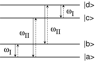
Figure 1: Schematic illustration of the eigenstates of the bipartite qubit-qubit system and of the allowed transitions characterized by the Bohr frequencies $\omega_{I}$ and $\omega_{II}$.

Inserting in Eq. (7) the structure of the jump operators given in Eqs. (10)-(13), the Markovian master equation can be cast in the following form:

$$\dot{\rho}(t) = -i\left[H_{S},\rho(t)\right]$$ (14)

$$+ \sum_{i=I}^{II}\sum_{l=1}^{2}\gamma_{i,\,ll}\left(J_{il}\rho(t)J_{il}^{\dagger}-\frac{1}{2}\left\{J_{il}^{\dagger}J_{il},\rho(t)\right\}\right)$$

$$+ \sum_{i=I}^{II}\sum_{l=1}^{2}\bar{\gamma}_{i,\,ll}\left(J_{il}^{\dagger}\rho(t)J_{il}-\frac{1}{2}\left\{J_{il}J_{il}^{\dagger},\rho(t)\right\}\right)$$

where, assuming that the two reservoirs are independent and each of them is in a thermal state, with temperatures $T_{1}$ and $T_{2}$ respectively, one has:

$$\gamma_{i,\,lm}=\int_{-\infty}^{+\infty}d\tau\mathrm{e}^{i\omega_{i}\tau}\left<B_{l}^{\dagger}(\tau)B_{m}(0)\right>,$$ (15)

and the Kubo-Martin-Schwinger relation

$$\bar{\gamma}_{i,\,ll}=\mathrm{e}^{-\omega_{i}/K_{B}T_{l}}{\gamma}_{i,\,ll}$$ (16)

holds [6]. The hypotesis of independent reservoirs we have made consists in assuming that $\left<B_{l}^{\dagger}(\tau)B_{m}(0)\right>=0$, i.e. $\gamma_{i,\,lm}=0$, when $l\neq m$.

Finally, by inserting Eqs. (10)-(13) into Eq. (14) and rearranging the terms, we obtain:

$$\dot{\rho}(t)=-i\left[H_{S},\rho(t)\right]$$ (17)

$$+c_{I}\left(|{a}\rangle\langle{b}|\rho(t)|{b}\rangle\langle{a}|-\frac{1}{2}\left\{|{b}\rangle\langle{b}|,\rho(t)\right\}\right)+c_{II}\left(|{a}\rangle\langle{c}|\rho(t)|{c}\rangle\langle{a}|-\frac{1}{2}\left\{|{c}\rangle\langle{c}|,\rho(t)\right\}\right)$$

$$+c_{I}\left(|{b}\rangle\langle{d}|\rho(t)|{d}\rangle\langle{b}|-\frac{1}{2}\left\{|{d}\rangle\langle{d}|,\rho(t)\right\}\right)+c_{II}\left(|{c}\rangle\langle{d}|\rho(t)|{d}\rangle\langle{c}|-\frac{1}{2}\left\{|{d}\rangle\langle{d}|,\rho(t)\right\}\right)$$

$$+\bar{c}_{I}\left(|{b}\rangle\langle{a}|\rho(t)|{a}\rangle\langle{b}|-\frac{1}{2}\left\{|{a}\rangle\langle{a}|,\rho(t)\right\}\right)+\bar{c}_{II}\left(|{c}\rangle\langle{a}|\rho(t)|{a}\rangle\langle{c}|-\frac{1}{2}\left\{|{a}\rangle\langle{a}|,\rho(t)\right\}\right)$$

$$+\bar{c}_{I}\left(|{d}\rangle\langle{b}|\rho(t)|{b}\rangle\langle{d}|-\frac{1}{2}\left\{|{b}\rangle\langle{b}|,\rho(t)\right\}\right)+\bar{c}_{II}\left(|{d}\rangle\langle{c}|\rho(t)|{c}\rangle\langle{d}|-\frac{1}{2}\left\{|{c}\rangle\langle{c}|,\rho(t)\right\}\right)$$

$$+c_{cr,I}\left(|{a}\rangle\langle{b}|\rho(t)|{d}\rangle\langle{c}|+|{c}\rangle\langle{d}|\rho(t)|{b}\rangle\langle{a}|\right)+c_{cr,II}\left(|{a}\rangle\langle{c}|\rho(t)|{d}\rangle\langle{b}|+|{b}\rangle\langle{d}|\rho(t)|{c}\rangle\langle{a}|\right)$$

$$+\bar{c}_{cr,I}\left(|{d}\rangle\langle{c}|\rho(t)|{a}\rangle\langle{b}|+|{b}\rangle\langle{a}|\rho(t)|{c}\rangle\langle{d}|\right)+\bar{c}_{cr,II}\left(|{d}\rangle\langle{b}|\rho(t)|{a}\rangle\langle{c}|+|{c}\rangle\langle{a}|\rho(t)|{b}\rangle\langle{d}|\right).$$

The decay rates $c_{i}$, and the cross terms $c_{cr,i}$ (with $i=I,II$), are given by:

$$c_{I} = \gamma_{I,11}\left(\cos\frac{\theta_{I}}{2}\cos\frac{\theta_{II}}{2}+\sin\frac{\theta_{I}}{2}\sin\frac{\theta_{II}}{2}\right)^{2}$$ (18)

$$+ \gamma_{I,22}\left(\cos\frac{\theta_{I}}{2}\sin\frac{\theta_{II}}{2}+\sin\frac{\theta_{I}}{2}\cos\frac{\theta_{II}}{2}\right)^{2},$$

$$c_{II} = \gamma_{II,11}\left(\cos\frac{\theta_{I}}{2}\sin\frac{\theta_{II}}{2}-\sin\frac{\theta_{I}}{2}\cos\frac{\theta_{II}}{2}\right)^{2}$$ (19)

$$+ \gamma_{II,22}\left(\cos\frac{\theta_{I}}{2}\cos\frac{\theta_{II}}{2}-\sin\frac{\theta_{I}}{2}\sin\frac{\theta_{II}}{2}\right)^{2},$$

$$c_{cr,I} = \gamma_{I,11}\left(\cos\frac{\theta_{I}}{2}\cos\frac{\theta_{II}}{2}+\sin\frac{\theta_{I}}{2}\sin\frac{\theta_{II}}{2}\right)^{2}$$ (20)

$$- \gamma_{I,22}\left(\cos\frac{\theta_{I}}{2}\sin\frac{\theta_{II}}{2}+\sin\frac{\theta_{I}}{2}\cos\frac{\theta_{II}}{2}\right)^{2},$$

$$c_{cr,II} = -\gamma_{II,11}\left(\cos\frac{\theta_{I}}{2}\sin\frac{\theta_{II}}{2}-\sin\frac{\theta_{I}}{2}\cos\frac{\theta_{II}}{2}\right)^{2}$$ (21)

$$+ \gamma_{II,22}\left(\cos\frac{\theta_{I}}{2}\cos\frac{\theta_{II}}{2}-\sin\frac{\theta_{I}}{2}\sin\frac{\theta_{II}}{2}\right)^{2},$$

The corresponding excitation rates $\bar{c}_{i}$, and the cross terms $\bar{c}_{cr,i}$, are obtained by substituting, in Eqs. (18)-(21), $\gamma_{i,ll}$ with the corresponding quantities $\bar{\gamma}_{i,ll}$: when the temperatures of the two reservoirs $T_{1}$ and $T_{2}$ are both zero, all this coefficients vanish, according to Eq. (16). Physically this means that there is no possibility to create excitations in the bipartite system due to the interaction with the reservoirs.

Let us conclude this section by reminding that the master equation has been derived in the framework of Born-Markov and rotating wave approximations. The last approximation is valid as long as the relaxation time of the system is much longer than the time characterizing its unitary dynamics [6]. Mathematically this is equivalent to assume that the coupling with the environment is weak enough to say that the relaxation rates are all much smaller than the smallest nonzero Bohr frequency relative to $H_{S}$, that is $\omega_{I}$.

4 Dynamics

The master equation given by Eq. (17), is equivalent to a system of coupled differential equation, the first four of which describe the time evolution of the populations of the dressed states $|{a}\rangle$, $|{b}\rangle$, $|{c}\rangle$ and $|{d}\rangle$, namely

$$\dot{\rho}_{aa}(t)=-\left(\bar{c}_{I}+\bar{c}_{II}\right)\rho_{aa}(t)+c_{I}\rho_{bb}(t)+c_{II}\rho_{cc}(t)$$

$$\dot{\rho}_{bb}(t)=\bar{c}_{I}\rho_{aa}(t)-\left(c_{I}+\bar{c}_{II}\right)\rho_{bb}(t)+c_{II}\rho_{dd}(t)$$

$$\dot{\rho}_{cc}(t)=\bar{c}_{II}\rho_{aa}(t)-\left(c_{II}+\bar{c}_{I}\right)\rho_{cc}(t)+c_{I}\rho_{dd}(t)$$

$$\dot{\rho}_{dd}(t)=\bar{c}_{II}\rho_{bb}(t)+\bar{c}_{I}\rho_{cc}(t)-\left(c_{I}+c_{II}\right)\rho_{dd}(t),$$ (22)

while the other equations describe the time evolution of the coherences:

$$\dot{\rho}_{ac}(t)=\left[i\omega_{II}-\frac{\left(c_{II}+2\bar{c}_{I}+\bar{c}_{II}\right)}{2}\right]\rho_{ac}(t)+c_{cr,I}\rho_{bd}(t)$$

$$\dot{\rho}_{bd}(t)=\left[i\omega_{II}-\frac{\left(2c_{I}+c_{II}+\bar{c}_{II}\right)}{2}\right]\rho_{bd}(t)+\bar{c}_{cr,I}\rho_{ac}(t)$$ (23)

$$\dot{\rho}_{ab}(t)=\left[i\omega_{I}-\frac{\left(c_{I}+\bar{c}_{I}+2\bar{c}_{II}\right)}{2}\right]\rho_{ab}(t)+c_{cr,II}\rho_{cd}(t)$$

$$\dot{\rho}_{cd}(t)=\left[i\omega_{I}-\frac{\left(c_{I}+2c_{II}+\bar{c}_{I}\right)}{2}\right]\rho_{cd}(t)+\bar{c}_{cr,II}\rho_{ab}(t)$$ (24)

$$\dot{\rho}_{ad}(t)=\left[i\omega_{da}-\frac{\left(c_{I}+c_{II}+\bar{c}_{I}+\bar{c}_{II}\right)}{2}\right]\rho_{ad}(t)$$

$$\dot{\rho}_{bc}(t)=\left[i\omega_{cb}-\frac{\left(c_{I}+c_{II}+\bar{c}_{I}++\bar{c}_{II}\right)}{2}\right]\rho_{bc}(t),$$ (25)

where $\omega_{da}=E_{d}-E_{a}$ and $\omega_{cb}=E_{c}-E_{b}$. The other coherences can be obtained by complex conjugation. In the following subsections we will discuss the existence of a stationary solution and we will bring to light the features characterizing the dynamics of the entanglement when both $T_{1}$ and $T_{2}$ are equal to zero.

4.1 Solution I: The stationary state

Let us look for the existence of the stationary solution by imposing $\dot{\rho}_{ii}=0$ ($\forall\,i\equiv\{a,b,c,d\}$) in Eqs. (4) and the normalization condition $Tr(\rho(t))=1$. In such a condition, after some calculations, it is possible to prove the existence of a stationary solution given by:

$$\rho_{aa,\,ST}=\frac{c_{I}c_{II}}{(c_{I}+\bar{c}_{I})(c_{II}+\bar{c}_{II})}$$

$$\rho_{bb,\,ST}=\frac{\bar{c}_{I}c_{II}}{(c_{I}+\bar{c}_{I})(c_{II}+\bar{c}_{II})}$$

$$\rho_{cc,\,ST}=\frac{c_{I}\bar{c}_{II}}{(c_{I}+\bar{c}_{I})(c_{II}+\bar{c}_{II})}$$

$$\rho_{dd,\,ST}=\frac{\bar{c}_{I}\bar{c}_{II}}{(c_{I}+\bar{c}_{I})(c_{II}+\bar{c}_{II})}$$ (26)

As it is immediate to see, when $T_{1}=T_{2}=0$ K, $\rho_{aa,\,ST}=1$, namely the stationary solution coincides with the ground state of the bipartite system. In view of Eq. (2), this implies the existence of a stationary entanglement traceable back to the presence of counter-rotating terms in the interaction Hamiltonian (see Eq. (1)) describing the coupling between the two two-state systems. We will discuss stationary entanglement in the next subsection.

4.2 Solution II: Entanglement dynamics at zero temperature

Let us consider now the analysis of the system dynamics when the temperatures of the two reservoirs, $T_{1}$ and $T_{2}$, are equal to $0$ K. Moreover let us restrict our attention to the case of exact resonance $\omega_{1}=\omega_{2}$ and in which the two environment have both flat spectra and are coupled with equal strength to the respective subsystems, which means that $\gamma_{I,11}=\gamma_{II,11}=\gamma_{I,22}=\gamma_{I,22}$. From Eqs. (5), (20) and (21), it is straightforward to show that in this case the cross coefficients $c_{cr,I}$ and $c_{cr,II}$ are both equal to zero, so that each coherence between the dressed states of the system evolves independently for the other ones.

Putting this condition into Eqs. (4) -(4), it is possible to show that their solution is:

$$\rho_{aa}(t)=1-\rho_{bb}(t)-\rho_{cc}(t)-\rho_{dd}(t),$$ (27)

$$\rho_{bb}(t)=\left(\rho_{bb}(0)+\rho_{dd}(0)\right)\mathrm{e}^{-c_{I}t}-\rho_{dd}(0)\mathrm{e}^{-(c_{I}+c_{II})t},$$ (28)

$$\rho_{cc}(t)=\left(\rho_{cc}(0)+\rho_{dd}(0)\right)\mathrm{e}^{-c_{II}t}-\rho_{dd}(0)\mathrm{e}^{-(c_{I}+c_{II})t},$$ (29)

$$\rho_{dd}(t)=\rho_{dd}(0)\mathrm{e}^{-(c_{I}+c_{II})t}$$ (30)

and

$$\rho_{ac}(t)=\mathrm{e}^{\left[i\omega_{II}-\frac{\left(c_{II}+2\bar{c}_{I}+\bar{c}_{II}\right)}{2}\right]t}\rho_{ac}(0)$$ (31)

$$\rho_{bd}(t)=\mathrm{e}^{\left[i\omega_{II}-\frac{\left(2c_{I}+c_{II}+\bar{c}_{II}\right)}{2}\right]t}\rho_{bd}(0)$$ (32)

$$\rho_{ab}(t)=\mathrm{e}^{\left[i\omega_{I}-\frac{\left(c_{I}+\bar{c}_{I}+2\bar{c}_{II}\right)}{2}\right]t}\rho_{ab}(0)$$ (33)

$$\rho_{cd}(t)=\mathrm{e}^{\left[i\omega_{I}-\frac{\left(c_{I}+2c_{II}+\bar{c}_{I}\right)}{2}\right]t}\rho_{cd}(0)$$ (34)

$$\rho_{ad}(t)=\mathrm{e}^{\left[i\omega_{da}-\frac{\left(c_{I}+c_{II}+\bar{c}_{I}+\bar{c}_{II}\right)}{2}\right]t}\rho_{ad}(0)$$ (35)

$$\rho_{bc}(t)=\mathrm{e}^{\left[i\omega_{cb}-\frac{\left(c_{I}+c_{II}+\bar{c}_{I}++\bar{c}_{II}\right)}{2}\right]t}\rho_{bc}(0)$$ (36)

Starting from the initial state

$$|{\psi(0)}\rangle=\sqrt{p}|{01}\rangle+\mathrm{e}^{i\varphi}\sqrt{1-p}|{10}\rangle,$$ (37)

$p$ being a non-negative real number $\leq 1$, and by taking into account that

$$\rho_{bb}(0)=\left|\mathrm{e}^{i\varphi}\sqrt{1-p}\,\cos\left(\frac{\theta_{II}}{2}\right)-\sqrt{p}\,\sin\left(\frac{\theta_{II}}{2}\right)\right|^{2},$$ (38)

$$\rho_{cc}(0)=\left|\mathrm{e}^{i\varphi}\sqrt{1-p}\,\sin\left(\frac{\theta_{II}}{2}\right)+\sqrt{p}\,\cos\left(\frac{\theta_{II}}{2}\right)\right|^{2},$$ (39)

$$\rho_{bc}(0) = \left(\mathrm{e}^{i\varphi}\sqrt{1-p}\,\cos\left(\frac{\theta_{II}}{2}\right)-\sqrt{p}\,\sin\left(\frac{\theta_{II}}{2}\right)\right)$$ (40)

$$\times\left(\mathrm{e}^{-i\varphi}\sqrt{1-p}\,\sin\left(\frac{\theta_{II}}{2}\right)+\sqrt{p}\,\cos\left(\frac{\theta_{II}}{2}\right)\right),$$

while $\rho_{ii}=0$ and $\rho_{ij}=0$ otherwise, it is possible to see that the density matrix describing the time evolution of the bipartite system at a generic instant of time $t$ assumes the following form:

$$\rho(t) = \rho_{aa}(t)|{a}\rangle\langle{a}|+\rho_{bb}(t)|{b}\rangle\langle{b}|+\rho_{cc}(t)|{c}\rangle\langle{c}|+\rho_{dd}(t)|{d}\rangle\langle{d}|$$ (41)

$$+\rho_{bc}(t)|{b}\rangle\langle{c}|+\rho_{cb}(t)|{c}\rangle\langle{b}|$$

To assess how much entanglement is stored in this bipartite quantum system at different instants of time we use the concurrence, a function introduced by Wootters [15], equal to $1$ for maximally entangled states and zero for separable states, defined as:

$$\mathcal{C}(t)=max(0,\sqrt{\lambda_{1}(t)}-\sqrt{\lambda_{2}(t)}-\sqrt{\lambda_{3}(t)}-\sqrt{\lambda_{4}(t)})$$ (42)

where $\{\lambda_{i}(t)\}$ are the eigenvalues of the matrix

$$R(t)=\rho(t)\tilde{\rho}(t),$$ (43)

with $\tilde{\rho}(t)$ given by $\tilde{\rho}(t)=\sigma_{y}\otimes\sigma_{y}\rho^{*}(t)\sigma_{y}\otimes\sigma_{y}$, $\sigma_{y}$ being the Pauli matrix, and $\rho(t)$ the density matrix representing the quantum state of the system. Inserting Eq. (41) into Eq. (43), it is possible to derive the time evolution of concurrence, studying in this way the features of the non-classical correlations characterizing the system of the two coupled qubits. More in details, it is possible to see that when the system is initially prepared in the factorized state $|{01}\rangle$ its dynamics is characterized by the existence of damped oscillations corresponding to the periodic appearance and disappearance of non-classical correlations between the two qubits. The oscillations in the concurrence are a direct signature of the well known oscillations of the single excitation between the two qubits, which are caused by the resonant terms in the qubit-qubit interaction. On the other hand the stationary entanglement at long times is a consequence of the fact that, due to the counter-rotating terms in the Hamiltonian in Eq. (1), the ground state of the system is not the unexcited state $\left|00\right>$, but the entangled state $|{a}\rangle$ in Eq. (2). From Eq. (4) it is straightforward to see that the smaller the coupling constant $\lambda$ the smaller the amount of stationary entanglement.

The system dynamics is even richer when the system is initially prepared in a state with two excitations or in an arbitrary superposition of the states $|{00}\rangle$ and $|{11}\rangle$, i.e.

$$|{\psi(0)}\rangle=\sqrt{p}|{00}\rangle+\mathrm{e}^{i\varphi}\sqrt{1-p}|{11}\rangle.$$ (44)

Also in this case $p$ is a non-negative real number $\leq 1$, while we have:

$$\rho_{aa}(0)=\left|\sqrt{p}\,\cos\left(\frac{\theta_{I}}{2}\right)-\mathrm{e}^{i\varphi}\sqrt{1-p}\,\sin\left(\frac{\theta_{I}}{2}\right)\right|^{2},$$ (45)

$$\rho_{dd}(0)=\left|\sqrt{p}\,\sin\left(\frac{\theta_{I}}{2}\right)+\mathrm{e}^{i\varphi}\sqrt{1-p}\,\cos\left(\frac{\theta_{I}}{2}\right)\right|^{2},$$ (46)

$$\rho_{ad}(0) = \left(\sqrt{p}\,\cos\left(\frac{\theta_{I}}{2}\right)-\mathrm{e}^{i\varphi}\sqrt{1-p}\,\sin\left(\frac{\theta_{I}}{2}\right)-\right)$$ (47)

$$\times\left(\sqrt{p}\,\sin\left(\frac{\theta_{I}}{2}\right)+\mathrm{e}^{-i\varphi}\sqrt{1-p}\,\cos\left(\frac{\theta_{I}}{2}\right)\right),$$

with $\rho_{ii}=0$ and $\rho_{ij}=0$ otherwise. With such an initial condition, the density matrix of the system at a generic instant of time assumes the form

$$\rho(t) = \rho_{aa}(t)|{a}\rangle\langle{a}|+\rho_{bb}(t)|{b}\rangle\langle{b}|+\rho_{cc}(t)|{c}\rangle\langle{c}|+\rho_{dd}(t)|{d}\rangle\langle{d}|$$ (48)

$$+\rho_{ad}(t)|{b}\rangle\langle{c}|+\rho_{da}(t)|{c}\rangle\langle{b}|.$$

Exploiting Eq. (44) (with $p=0$) as well as Eqs. (45)-(48) it easy to derive the time evolution of the concurrence of the two qubits. Figure 3 shows that, apart from the oscillations of the entanglement due to the oscillations of the excitation in the one-excitation subspace, the behaviour of the concurrence is characterized by the phenomena of sudden birth and sudden death of the entanglement already found by Ficek and Tanas [14] for the scenario of two interacting qubits. While the phenomenon entanglement sudden death, i.e., the complete disentanglement of the system in a finite time, is quite well understood and is a feature common to any dissipative two-qubits dynamics, provided the system starts from the proper initial state [11, 12], the occurrence of stationary entanglement is a phenomenon usually ascribed to the presence of a reservoir which is common to the two parts of the bipartite system [14, 16]. What we have proved here is that the same phenomenon can occur even in the presence of independent reservoirs for the two qubits, provided the interaction Hamiltonian between the two qubits contains also the counter-rotating terms which are usually neglected in the study of the dynamics. This is due to the fact that, in the weak damping limit, the quantum jumps occur between eigenstates of the system Hamiltonian and to the fact that, due to the presence of counter-rotating terms in the two-qubit interaction, the ground state of the system is an entangled state, as we have seen before.

Figure 2: Concurrence of the two qubits as a function of time $t$ (in units of $10*(\lambda)^{-1})$. The initial state is $|{01}\rangle$, the parameters assume the values $\omega_{1}/\lambda=\omega_{2}/\lambda=10$, $T_{1}=T_{2}=0$ K, $\gamma_{I,11}/\lambda=\gamma_{II,11}/\lambda=\gamma_{I,22}/\lambda=\gamma_{I,22}/\lambda=0.01$.

Figure 3: Concurrence of the two qubits as a function of time $t$ (in units of $10*(\lambda)^{-1})$. The initial state is $|{11}\rangle$, the parameters assume the values $\omega_{1}/\lambda=\omega_{2}/\lambda=10$, $T_{1}=T_{2}=0$ K, $\gamma_{I,11}/\lambda=\gamma_{II,11}/\lambda=\gamma_{I,22}/\lambda=\gamma_{I,22}/\lambda=0.01$.

5 Discussion and Conclusive Remarks

To summarize, we have presented a microscopic derivation of the Markovian master equation in the weak damping limit governing the time evolution of two interacting two-state systems, each of them coupled to independent bosonic reservoirs, and we have studied the time evolution of the entanglement between the two qubits for various initial conditions of the bipartite system.

The behaviour of the concurrence is consistent with the results of the literature, showing the occurrence of entanglement sudden death for some initial states and of stationary entanglement for any initial state. The presence of stationary entanglement which is not washed away from dissipation is perhaps the most important result of our analysis. Indeed this feature is usually ascribed to the presence of a common reservoir which correlates the two parts of the bipartite system. Instead we have shown here that stationary entanglement can occur also due to the interaction between the two parts, provided their interaction is described in a complete way which includes the counter-rotating terms in their interaction Hamiltonian. We feel that our approach could help in understanding the role of energy non-conserving terms in the dissipative dynamics of open bipartite quantum systems. From this point of view more is expected from the analysis of the cases with reservoirs at different temperatures or with non-flat spectrum, in the framework of a non-Markovian extension of the master equation presented here. These points will be the subject of our future work.

References

References

• [1] Haroche S. and Raimond J.M., 2006 Exploring the quantum: atom, cavities and photons (Oxford: Oxford University Press).
• [2] Wheeler J.A. and Zurek W.H., 1983 Quantum Theory of Measurement (Princeton: Princeton University Press).
• [3] Nielsen M.A. and Chuang I.L., 2000 Quantum Computation and Quantum Information (Cambridge: Cambridge University Press).
• [4] Cohen-Tannoudji C. et al., 1998 Atom-Photon Interactions (New York: John Wiley)
• [5] Gardiner C.W. and Zoller P., 2000 Quantum Noise (Berlin: Springer)
• [6] Breuer H.-P. and Petruccione F., 2002 The Theory of Open Quantum Systems (Oxford: Oxford University Press)
• [7] Scala M., Militello B., Messina A., Piilo J. and Maniscalco S., 2007 Phys. Rev. A 75, 013811.
• [8] Scala M., Militello B., Messina A., Maniscalco S., Piilo J. and Suominen K.-A., 2007 J. Phys. A: Math. and Theor. 40, 14527.
• [9] Scala M., Militello B., Messina A., Maniscalco S., Piilo J. and Suominen K.-A., 2008 Phys. Rev. A 77, 043827.
• [10] Migliore R., Yuasa K., Nakazato H., and Messina A., 2006 Phys. Rev. B 74, 104503.
• [11] Yu T., Eberly J. H., 2004 Phys. Rev. Lett. 93, 140404; Yu T., Eberly J. H., 2006 Phys. Rev. Lett. 97, 140403.
• [12] Bellomo B., Lo Franco R., Compagno G., 2007 Phys. Rev. Lett. 99, 160502; Bellomo B., Lo Franco R., Compagno G., 2008 Phys. Rev. A 77 032342.
• [13] Paladino E., Sassetti M., Falci G., 2004 Chemical Physics, 296 325; Paladino E., Sassetti M., Falci G., Weiss U., 2008 Phys. Rev. B 77, 041303.
• [14] Tanas R., Ficek Z., 2004 J. Opt. B Quantum Semiclass. Opt. 6, S90; Ficek Z., Tanas R., 2006 Phys. Rev. A, 74, 024304.
• [15] Wootters W.K., 1998 Phys. Rev. Lett. 80, 2245.
• [16] Nicolosi S., Napoli A., Messina A., Petruccione F., 2004 Phys. Rev. A, 70 022511.