Current status of carlomat, a program for automatic computation of lowest order cross sections

Abstract

The current status of carlomat, a program for automatic computation of the lowest order cross sections of multiparticle reactions is described, the results of comparisons with other multipurpose Monte Carlo programs are shown and some new results on $e^{+}e^{-}\rightarrow b\bar{b}b\bar{b}u\bar{d}d\bar{u}$ are presented.

1 MOTIVATION

Many interesting aspects of the Standard Model (SM) and models beyond it can be studied through investigation of reactions involving a few heavy particles at a time. Owing to the high energy and luminosity such reactions will be copiously observed at particle colliders such as the Large Hadron Collider (LHC), or the International Linear Collider (ILC) [1]. As the heavy particles are usually unstable, they almost immediately decay leading to reactions with several particles in the final state. Already in the lowest order of SM matrix elements of such multiparticle reactions receive contributions typically from many thousands of the Feynman diagrams, most of which constitute background to the “signal diagrams” representing the interesting subprocesses of production and decay of those heavy particles. Because of the large number of Feynman diagrams involved, reliable SM predictions for such reactions can be obtained only through a fully automated calculational process.

To be more specific, let us consider, e.g. a reaction of associated production of the top quark pair and Higgs boson at the ILC

$$e^{+}e^{-}\rightarrow t\bar{t}H.$$ (1)

Because its cross section is by far dominated by the Higgsstrahlung off the top quark line, reaction (1) can be used to measure the top–Higgs Yukawa coupling [2]. As the top and antitop decay, even before they hadronize, predominantly into $bW^{+}$ and $\bar{b}W^{-}$, respectively, and the Higgs boson, dependent on its mass $m_{H}$, decays mostly either into a $b\bar{b}$-quark pair or an electroweak (EW) gauge boson pair and the EW bosons subsequently decay, each into a fermion–antifermion pair, reaction (1) will lead to reactions with either 8 or 10 fermions in the final state. If $m_{H}<140$ GeV, which is favoured by the direct searches at LEP [3] and theoretical constrains in the framework of SM [4], then the Higgs boson would decay mostly into a $b\bar{b}$-quark pair resulting in reactions of the form

$$e^{+}e^{-}\;\;\rightarrow\;\;b\bar{b}b\bar{b}f_{1}\bar{f^{\prime}_{1}}f_{2}\bar{f^{\prime}_{2}},$$ (2)

where $f_{1},f^{\prime}_{2}=\nu_{e},\nu_{\mu},\nu_{\tau},u,c$ and $f^{\prime}_{1},f_{2}=e^{-},\mu^{-},\tau^{-},d,s$ are the decay products of the $W$-bosons coming from decays of the $t$- and $\bar{t}$-quark. Thus, in this case reaction (1) can be detected in any of the following channels: the leptonic, semileptonic and hadronic channels, as represented by the reactions

$$e^{+}e^{-} \rightarrow b\bar{b}b\bar{b}\tau^{+}\nu_{\tau}\mu^{-}\bar{\nu}_{\mu},$$ (3)

$$e^{+}e^{-} \rightarrow b\bar{b}b\bar{b}u\bar{d}\mu^{-}\bar{\nu}_{\mu},$$ (4)

$$e^{+}e^{-} \rightarrow b\bar{b}b\bar{b}u\bar{s}d\bar{c},$$ (5)

respectively. Taking into account both the EW and quantum chromodynamics (QCD) lowest order contributions in the unitary gauge, with the neglect of the Yukawa couplings of the fermions lighter than $c$ quark and $\tau$ lepton, there are 21 214, 26 816 and 39 342 Feynman diagrams of reactions (3), (4) and (5), respectively. If both $W^{+}$ and $W^{-}$ decay into quarks of the same family we obtain, e.g. the reaction

$$e^{+}e^{-} \rightarrow b\bar{b}b\bar{b}u\bar{d}d\bar{u}$$ (6)

which, neglecting the light fermion masses, receives contributions from 185 074 Feynman diagrams. Most of the diagrams comprise background to the 20 signal diagrams representing resonant production and decay of the top quark pair and Higgs boson. For illustration, the representative signal diagrams of reaction (6) are shown in Fig. 1.

Figure 1: Representative signal Feynman diagrams of reaction (6) in the unitary gauge. The remaining diagrams are obtained by all possible permutations of the two $b$ and two $\bar{b}$ lines. The Higgs boson coupling to electrons has been neglected.

There exists several multipurpose Monte Carlo (MC) generators such as HELAC/PHEGAS [5], AMEGIC++/Sherpa [6], O’Mega/Whizard [7], MadGraph/MadEvent [8], ALPGEN [9], or CompHEP/CalcHEP [10]. However, one may encounter problems while trying to obtain reliable SM predictions for multiparticle reactions as (3)–(5), not to mention reaction (6), with publicly available versions of the generators.

In this lecture, the current status of carlomat, a new program for automatic computation of the lowest order cross sections of multiparticle reactions is described, the results of comparisons with other multipurpose MC programs are shown and some new results on reaction (6) are presented.

2 A PROGRAM

carlomat is a program written in Fortran 90/95. It generates the matrix element for a user specified process and phase space parametrizations, which are later used for the multichannel MC integration of the lowest order cross sections and event generation. The program takes into account both the EW and QCD lowest order contributions. Particle masses are not neglected in the program. The number of external particles is limited to 12 and only the SM is currently implemented in the program.

carlomat works according to the following scheme. User specifies the process he wants to have calculated. Then topologies for a given number of external particles are generated and checked against Feynman rules which have been coded in the program. In this process, helicity amplitudes, the colour matrix and phase space parametrizations are generated. Finally, they are copied to another directory where the numerical program can be executed.

2.1 Generation of topologies

Let us consider models with triple and quartic couplings. The process of generation of topologies starts with 1 topology of a 3 particle process that is depicted in Fig. 2.

Figure 2: The single topology of a 3 particle process.

The 4 topologies of a 4 particle process which are depicted in Fig. 3 are obtained by attaching line No. 4 to each line and to the vertex of the graph in Fig. 2.

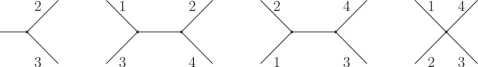
Figure 3: The topologies of a 4 particle process.

Then the 25 topologies of a 5 particle process are obtained by attaching line No. 5 to each line, including the internal ones, and to each triple vertex of the graphs in Fig. 3.

The number of topologies grows dramatically with the number of external particles.

No. of particles	No. of topologies
6	220
7	2 485
8	34 300
9	559 405
10	10 525 900
11	224 449 225

For a process with $n$ external particles, topologies for $n-1$ particles are generated recursively and then, while adding the $n$-th particle, the program checks whether a topology results in a Feynman diagram or not. Topologies can be generated and stored on a disk prior to the program execution.

2.2 Feynman diagrams

Actual external particles are assigned to lines $1,2,3,...,n$ in a strict order. Each topology is divided into two parts which are separately checked against the Feynman rules. Two or three, external lines are joined by means of a triple or quartic, vertex of the implemented model. In this way an off shell particle, which is represented by a spinor or polarization vector, is created. The off shell particles and/or external particles are joined in this way until the two parts of a considered topology are completely covered. If they match into a propagator then the topology is accepted. Once the topology has been accepted, the ‘longer’ part of it is further divided so that the Feynman diagram is made of 3 or 4 parts, joint to form a triple or quartic vertex of the model. Particles defined for one Feynman diagram are used as building blocks of other Feynman diagrams. The number of building blocks generated in carlomat is usually smaller than in MadGraph.

When the diagram is created, the corresponding ‘particles’ are used to construct the helicity amplitude, colour factor (matrix) and phase space parametrization which are stored on the disk. Once all the topologies have been checked subroutines for calculating the matrix element, colour matrix and phase space integration are written.

2.3 Helicity amplitudes

The helicity amplitudes are computed using the routines developed for MC programs ee4fgamma [11] and eett6f [12] which have been improved and tailored to meet needs of the automatic generation of amplitudes. In order to speed up the computation the MC summing over helicities has been implemented in the program. However, explicit summing over helicities is also possible. While doing so, spinors or polarization vectors representing particles, both on- and off-shell ones, are computed only once, for all the helicities of the external particles they are made of, and stored in arrays, which is a novel feature with respect to other programs, e.g. MadGraph.

Possible poles in the propagators of unstable particles are regularized by constant widths which are introduced through the complex mass parameters

$$M_{B}^{2}\! =\! m_{B}^{2}-im_{B}\Gamma_{B},\qquad B=W,Z,H,$$

$$\qquad M_{t} = \sqrt{m_{t}^{2}-im_{t}\Gamma_{t}},$$ (7)

which replace masses in the corresponding propagators

$$\Delta_{F}^{\mu\nu}(q)\! = \!\frac{-g^{\mu\nu}+q^{\mu}q^{\nu}/M_{V}^{2}}{q^{2}-M_{V}^{2}},$$

$$\Delta_{F}(q)\! = \!\frac{1}{q^{2}-M_{H}^{2}},\qquad S_{F}(q)=\frac{/\!\!\!q+M_{t}}{q^{2}-M_{t}^{2}},$$

both in the $s$- and $t$-channel Feynman diagrams. Propagators of a photon and gluon are taken in the Feynman gauge. The EW mixing parameter may be defined either real, referred to as the fixed width scheme (FWS), or complex, referred to as the complex mass scheme (CMS)

$$\sin^{2}\theta_{W}=1-\frac{m_{W}^{2}}{m_{Z}^{2}}\quad{\rm or}\quad\sin^{2}\theta_{W}=1-\frac{M_{W}^{2}}{M_{Z}^{2}}.$$

The colour matrix is calculated only once at the beginning of execution of the numerical program after having reduced its size with the use of the SU(3) algebra properties.

2.4 Phase space integration

A dedicated phase space parametrization is generated for each Feynman diagram. Mappings of the Breit-Wigner shape of the propagators of unstable particles and $\sim 1/s$ behaviour of the photon and gluon propagators are performed. Dedicated treatment of soft and collinear external photons, as well as $t$-channel photon/gluon exchange is envisaged.

The phase space parametrizations are incorporated into a multichannel MC integration routine for calculating total and differential cross sections. The integration is performed iteratively. It starts with equal weights for all the kinematical channels and the weights with which each kinematical channel contributes to the integral are determined anew after every iteration. carlomat can be used as MC generator of unweighted events as well.

3 TESTS

Matrix elements of many reactions with 6 particles and several reactions with 7 particles in the final state have been checked against MadGraph for randomly selected sets of momenta. An agreement better than 13 digits has been found.

Total cross sections of reactions $e^{+}e^{-}\rightarrow$ 4 fermions and $e^{+}e^{-}\rightarrow$ 4 fermions and a photon have been checked against ee4fgamma [11], and of $e^{+}e^{-}\rightarrow$ 6 fermions, relevant for the top quark pair production and decay, have been compared with eett6f. The results have agreed within one standard deviation of the MC integration.

Moreover, checks against other MC programs have been made. Cross sections of the following top quark pair production reactions at the ILC:

$$e^{+}e^{-} \rightarrow b\bar{b}u\bar{d}d\bar{u},$$ (8)

$$e^{+}e^{-} \rightarrow b\bar{b}u\bar{d}e^{-}\bar{\nu}_{e},$$ (9)

$$e^{+}e^{-} \rightarrow b\bar{b}\nu_{e}e^{+}\mu^{-}\bar{\nu}_{\mu},$$ (10)

$$e^{+}e^{-} \rightarrow b\bar{b}\nu_{\mu}\mu^{+}\mu^{-}\bar{\nu}_{\mu}$$ (11)

computed with carlomat are compared against of the corresponding results of HELAC/PHEGAS and AMEGIC++ [13] in Table 1. The cuts and initial parameters are those of [13] and, as in [13], the cross sections have been calculated with $10^{6}$ calls in the MC integration, before the cuts have been applied.

Table 1: Cross sections in fb of (8)–(11) at $\sqrt{s}=360$ GeV (first row) and $\sqrt{s}=500$ GeV (second row). The cuts and initial parameters are as those of [13]. The numbers in parentheses show the uncertainty of the last decimals.

Reac.	carlomat	AMAGIC++	HELAC
(8)	32.98(11)	32.90(15)	33.05(14)
	50.31(19)	49.74(21)	50.20(13)
(9)	11.448(26)	11.460(36)	11.488(15)
	17.424(56)	17.486(66)	17.492(41)
(10)	3.843(5)	3.847(15)	3.848(7)
	5.856(11)	5.865(24)	5.868(10)
(11)	3.837(5)	3.808(16)	3.861(19)
	5.834(10)	5.840(30)	5.839(12)

Satisfactory agreement also for all the other cross sections presented in [13] for about 80 reactions has been found. However, for some reactions containing gluons, or $e^{+}e^{-}$ pair in the final state, more calls had to be used in carlomat in order to match the corresponding precision of [13], as the appropriate mappings have not yet been implemented in the program. Cross sections of reaction (4) without the gluon exchange contributions computed with carlomat and Whizard are compared in Table 2. Again a satisfactory agreement can be seen.

Table 2: Cross sections in ab of (4) without the gluon exchange contributions calculated with carlomat and Whizard. The cuts and initial parameters are as those of [14]. The numbers in parentheses show the uncertainty of the last decimal.

$\sqrt{s}$ [GeV]	carlomat	Whizard
500	7.80(3)	7.76(2)
800	66.8(1)	67.3(1)
1000	61.4(1)	61.8(2)
2000	28.5(1)	28.1(3)

4 SAMPLE RESULTS

The capability of carlomat to handle multiparticle reactions with large numbers of the Feynman diagrams was demonstrated in [14], where the off resonance background effects in the associated top quark pair and Higgs boson production at the linear $e^{+}e^{-}$ collider were studied. In [14], the effects were shown in reactions (3)–(5). Here, we will address the question of the off resonance background contributions to the associated top quark pair and Higgs boson production in reaction (6) which is the hadronic detection channel of (1) that, in the unitary gauge and neglecting the Yukawa couplings to light fermions, receives contributions from 185 074 lowest order Feynman diagrams.

As in [14], let us identify jets with their original partons and define the following cuts on an angle between a quark and a beam and an angle between two quarks

$$5^{\circ}<\theta(q,\mathrm{beam})<175^{\circ},\qquad\theta(q,q^{\prime})>10^{\circ}$$ (12)

and a cut on a quark energy

$$E_{q}>15\;{\rm GeV},$$ (13)

which should allow to detect events with 8 separate jets. Moreover, in order to reconstruct $W$ bosons, top quarks and the Higgs boson let us assume 100% efficiency of $b$ tagging and impose the following invariant mass cuts:
a cut on the invariant mass of two non $b$ jets

$$60\;{\rm GeV}<\left[\left(p_{\sim b_{1}}+p_{\sim b_{2}}\right)^{2}\right]^{1/2}<90\;{\rm GeV},$$ (14)

a cut on the invariant mass of a $b$ jet, $b_{1}$, and two non $b$ jets, $b_{\sim b_{1}},b_{\sim b_{2}}$,

$$\left|\left[\left(p_{b_{1}}+p_{\sim b_{1}}+p_{\sim b_{2}}\right)^{2}\right]^{1/2}-m_{t}\right|<30\;{\rm GeV}$$ (15)

and an invariance mass cut on two $b$ jets, $b_{3}$ and $b_{4}$,

$$\left|\left[\left(p_{b_{3}}+p_{b_{4}}\right)^{2}\right]^{1/2}-m_{h}\right|<m_{bb}^{\rm cut},$$ (16)

with $m_{bb}^{\rm cut}=20$ GeV, 5 GeV, 1 GeV.

The total cross section of reaction (6) calculated with the complete set of the lowest order Feynmamn diagrams, $\sigma_{\rm all}$, and with the 20 signal diagrams, representatives of which are depicted in Fig. 1, $\sigma_{\rm sig.}$, with cuts (12)–(16) are shown in Table 3. The initial parameters used are those of [14].

Table 3: The cross sections $\sigma_{\rm all}$ and $\sigma_{\rm sig.}$ of (6) for 3 different values of the invariant mass cut $m_{bb}^{\rm cut}$ of (16). The other cuts are given by (12)–(15) and initial parameters used are as those of [14]. The numbers in parentheses show the uncertainty of the last decimal.

$\sqrt{s}$ [GeV]	$m_{bb}^{\rm cut}$ [GeV]	$\sigma_{\rm all}$ [ab]	$\sigma_{\rm sig.}$ [ab]
500	20	13.46(5)	8.72(1)
	5	10.12(4)	8.70(1)
	1	8.98(4)	8.67(1)
800	20	164.5(4)	128.6(1)
	5	139.5(4)	128.2(1)
	1	129.6(2)	127.7(1)
1000	20	137.9(3)	109.2(1)
	5	117.7(5)	109.1(1)
	1	110.6(5)	108.6(1)
2000	20	44.2(2)	36.17(4)
	5	38.2(2)	36.27(4)
	1	36.5(1)	36.14(4)

We see that invariant mass cut (16), which has been imposed in order to identify the $b\bar{b}$ quark pair coming from the Higgs boson decay, reduces the off resonance background very efficiently while it practically does not alter the signal cross section.

5 CONCLUSIONS AND OUTLOOK

carlomat can be used for automatic computation of cross sections of multiparticle reactions as it has been demonstrated in [14] and in Section 4. It can be used as an MC generator of unweighted events, too.

In spite of all the successful checks presented in Section 3, further thorough comparisons with other existing MC generators still should be done.

Interfaces to PDF’s, or ISR within the structure function approach are practically ready. Interfaces to parton shower and hadronization programs should be worked on. Extensions of SM can be implemented and the corresponding lowest order cross sections can be calculated in a fully automatic way.

Leading SM radiative corrections can be implemented, if corresponding subroutines are provided as it was done, e.g. in [15], where factorizable EW $\cal{O}(\alpha)$ corrections were included for reactions $e^{+}e^{-}\rightarrow$ 6 fermions relevant for the top quark pair production and decay at a linear $e^{+}e^{-}$ collider.

References

-
[1]
J. Brau, Y. Okada, N. Walker, et al.,
arXiv:0712.1950;
J.A. Aguilar-Saavedra, et al., arXiv:hep-ph/0106315;
T. Abe, et al., arXiv:hep-ex/0106056;
K. Abe, et al., arXiv:hep-ph/0109166. - [2] A. Djouadi, J. Kalinowski, P.M. Zerwas, Mod. Phys. Lett. A7 (1992) 1765; Z. Phys C54 (1992) 255.
- [3] R. Barate, et al., Phys. Lett. B565 (2003) 61.
-
[4]
The LEP Collaborations and the LEP electroweak
working group, arXiv:hep-ex/0612034v2, and references therein;
Ch. Parkes, International Conference on High Energy Physics, July 2006, http://lephiggs.web.cern.ch/;
B. Kilminster, arXiv:hep-ex/0611001, in Moscow 2006, ICHEP, pp. 750-753. -
[5]
A. Kanaki, C.G. Papadopoulos, Comput. Phys. Commun.
132 (2000) 306;
C.G. Papadopoulos, Comput. Phys. Commun. 137 (2001) 247. C.G. Papadopoulos, M. Worek, in Tsukuba 2006, Deep inelastic scattering, pp. 507–510, arXiv: hep-ph/0606320. -
[6]
F. Krauss, R. Kuhn, G. Soff, JHEP 0202 (2002) 044;
T. Gleisberg, S. Höche, F. Krauss, A. Schälicke, S. Schumann, J.C. Winter, JHEP 0402 (2004) 056. -
[7]
M. Moretti, T. Ohl, J. Reuter,
arXiv:hep-ph/0102195-rev;
W. Kilian, T. Ohl, J. Reuter, arXiv:0708.4233. -
[8]
T. Stelzer, W.F. Long, Comput. Phys. Commun. 81
(1994) 357;
F. Maltoni, T. Stelzer, JHEP 02 (2003) 027. - [9] M.L. Mangano, M. Moretti, F. Piccinini, R. Pittau, A. Polosa, JHEP 0307 (2003) 001.
-
[10]
E. Boos et al. Nucl. Instrum. Meth. A534 (2004) 250;
A. Pukhov, arXiv:hep-ph/0412191. - [11] K. Kołodziej, F. Jegerlehner, Comput. Phys. Commun. 159 (2004) 106.
- [12] K. Kołodziej, Comput. Phys. Commun. 151 (2003) 339.
- [13] T. Gleisberg, et al., Eur. Phys. J C34 (2004) 173.
- [14] K. Kołodziej, S. Szczypiński, Nucl. Phys. B801 (2008) 153.
- [15] K. Kołodziej, A. Staroń, A. Lorca, T. Riemann, Eur. Phys. J C46 (2006) 357.