Photo- and Electroproduction of the Hypertriton on ³He

Abstract

Differential cross sections of the photo- and electroproduction of the hypertriton have been calculated by utilizing modern nuclear wave functions and the elementary operator of KAON-MAID. It is found that a proper treatment of Fermi motion is essential for the two processes. While the average momentum approximation can partly simulate the Fermi motion in the process, the “frozen nucleon” assumption yields very different results, especially at lower energies. The Coulomb effect induced by the interaction between the positively charged kaon and the hypertriton is found to be negligible. The influence of higher partial waves is also found to be relatively small, in contrast to the finding of the previous work. The off-shell assumption is found to be very sensitive in the case of electroproduction rather than in photoproduction. It is shown that the few available experimental data favor the assumption that the initial nucleon is off-shell and the final hyperon is on-shell. This seems to be reasonable, since the hyperon in the hypertriton is less bound than the nucleon in the initial ³He nucleus. The effect of the missing resonance $D_{13}(1895)$ is more profound in the longitudinal cross sections. Excluding this resonance reduces the longitudinal cross sections by one order of magnitude, but does not change the effects of various off-shell assumptions on the cross sections.

I Introduction

The hypertriton is a bound state consisting of a proton, a neutron, and a $\Lambda$ hyperon. Although a hypertriton consisting of a proton, a neutron, and a $\Sigma^{0}$ hyperon could exist, no experimental information is available at present sighyp ; Afnan ; Dover . Therefore, we will use the term “hypertriton” to denote the $\Lambda$-hypertriton in the following. Interest in the hypertriton is mainly due to the fact that it is the lightest and the loosely bound hypernucleus. The separation energy into a $\Lambda$ and a deuteron is only $0.13\pm 0.05$ MeV Juric:1973zq , while the total binding energy is 2.35 MeV. Being the lightest hypernucleus, the hypertriton is obviously the first system in which the $YN$ potential, including the interesting $\Lambda$-$\Sigma$ conversion, can be tested in the nuclear medium. This is also supported by the fact that neither the $\Lambda N$ nor the $\Sigma N$ interactions possesses sufficient strength to produce a bound two-body system, while on the other hand the available $YN$ scattering data are still extremely poor. Therefore the hypertriton is expected to play an important role in hypernuclear physics similar to that of the deuteron in conventional nuclear physics. Due to experimental difficulties, however, the existing information on the hypertriton is mostly from old measurements oldi .

Recently, theoretical investigation of the hypertriton properties have drawn considerable attentions in the nuclear physics community miyagawa93 ; miyagawa95 ; hyp_properties . The Bochum group miyagawa93 has investigated the hypertriton by using various $YN$ and $NN$ potentials. Interestingly, when the Jülich hyperon-nucleon potential in the one-boson-exchange (OBE) parameterization (model $\tilde{\rm A}$ of Ref. juelich ) combined with various realistic $NN$ interactions were used, then the hypertriton turned out to be unbound. Only an increase by about 4% in the Jülich potential can bring the hypertriton back to a bound state. However, the use of the Nijmegen hyperon-nucleon potential in the same calculation nijmegen89 leads to a bound hypertriton. This fact indicates that significant improvement in the hyperon-nucleon force sector is strongly needed.

In principle, the hypertriton could be produced by employing hadronic properties such as stopped and low momentum kaon induced reactions, A$(K,\pi)$B and A$(\pi,K)$B. Another possibility to obtain hypertriton is by utilizing the proton-deuteron collision

$$p+d\to K^{+}+{{}^{3}_{\Lambda}{\rm H}}~{}.$$ (1)

Komarov et al. have studied this process theoretically at incident proton energies $T_{p}=1.13-3.0$ GeV and found that the cross section is on the order of 1 nb, at most komarov . This result has been refined in Ref. Gardestig:1996zz by using a two-step model and the differential cross section is found to be much smaller than 1 nb/sr.

Because the electromagnetic beams (electrons or real photons) are well understood, clean, and well under control, the use of the electromagnetic processes has, however, a competing advantage compared to the hadronic ones. More than one decade ago one of the authors has estimated the cross section of the hypertriton photoproduction

$$\gamma+{{}^{3}{\rm He}}\to K^{+}+{{}^{3}_{\Lambda}{\rm H}}~{},$$ (2)

and investigated the effects of the off-shell assumption and Fermi motion on this process mart98 ; mart_thesis . This has been performed by using the wave function of ³He obtained as a solution of the Faddeev equations with the Reid soft core potential kim , and a simple hypertriton wave function developed in Ref. congleton , along with the elementary operator from Williams et al. williams . The result showed that the cross sections are predicted to be on the order of 1 nb and drop quickly as a function of the kaon scattering angle. Eight years later three experimental data points on the hypertriton electroproduction

$$e+{{}^{3}{\rm He}}\to e^{\prime}+K^{+}+{{}^{3}_{\Lambda}{\rm H}}~{},$$ (3)

at $\theta_{K}^{\rm c.m.}=2.7^{\circ},9.5^{\circ}$, and $18.9^{\circ}$, were published by Dohrmann et al. Dohrmann:2004xy . Although this process utilizes electrons (virtual photons), and therefore is different from the process given by Eq. (2), the result shows a surprising phenomenon, i.e., the angular distribution of the differential cross section shows an almost flat structure. An extrapolation of the photoproduction result to the finite $k^{2}$ region is only able to reproduce the trend of the first two data points and, on the other hand, underpredicts the last data point by one order of magnitude note_on_dohrmann . This is in contrast to the process

$$e+{{}^{4}{\rm He}}\to e^{\prime}+K^{+}+{{}^{4}_{\Lambda}{\rm H}}~{},$$ (4)

reported by the same experiment Dohrmann:2004xy , for which the cross section decreases smoothly and nicely fits the prediction note_on_dohrmann1 .

The present work has been greatly motivated by the facts described above. In the present work we shall only focus on the photo- and electroproduction of the hypertriton and leave the electroproduction of ${}^{4}_{\Lambda}{\rm H}$ for the future consideration. For this purpose we shall use the modern nuclear wave functions nijmegen93 ; miyagawa93 as well as the frequently used elementary operator KAON-MAID kaon-maid to study the effects of the various off-shell assumptions, Fermi motion, and Coulomb interaction between the exited kaon and the hypertriton, on the calculated differential cross sections. Recently, this elementary operator has been used to investigate the final states $YN$ and $KN$ interactions in kaon photoproduction off a deuteron as well as to investigate the possibility of extracting the elementary process $N(\gamma,K^{0})Y$ from this process at the quasi-free-scattering kinematics YaM99 . The elementary operator is given in a unique form that is completely frame independent, since it can be expressed in terms of the Mandelstam variables $s$, $u$, and $t$, or the four-momenta of the photon, nucleon, kaon, and hyperon. Furthermore, the operator does not contain the photon-polarization-vector $\epsilon^{\mu}$ and spin-operator $\sigma^{(n)}$ terms. This guarantees the analytical continuation of the elementary amplitude and enables us to use different off-shell assumptions. Thus, the result would provide us with a refined calculation of the hypertriton photoproduction and a direct comparison with the electroproduction data.

This paper is organized as follows: In Section II we shall briefly review the properties of the elementary operator used in this work. Section III presents the formalism of the nuclear operator along with its relation to the elementary operator and to the nuclear cross sections. We shall present and discuss the results of our calculations in Section IV. Section V summarizes our findings. A few important notes on the elementary amplitudes, the anti-symmetry factor of the nuclear wave functions, and some kinematical relations are given in the Appendices.

II Properties of the Elementary Operator

Since photoproduction is only a special case of electroproduction, we will only consider the latter in our formalism. The results for photoproduction are obtained by setting the virtual photon momentum to zero. The elementary process for electroproduction of a kaon and a hyperon on the nucleon target can be written as

$$e(k_{\rm i})+N(p_{N})\longrightarrow e^{\prime}(k_{\rm f})+K(q_{K})+Y(p_{Y})~{}.$$ (5)

To describe this process we make use of an isobar model, because by utilizing this model the elementary amplitudes can be written in term of a frame independent operator which is required to include the Fermi motion in the nucleus. The process is schematically shown in Fig. 1, where it is assumed that the electromagnetic interaction is mediated by one photon exchange. The elementary transition operator can be written as

$${M}_{\rm fi} = \epsilon_{\mu}\,J^{\mu}~{}=~{}\bar{u}(\mbox{\boldmath${p}$}_{Y})\,\sum_{i=1}^{6}\,A_{i}(k^{2},s,t,u)\,M_{i}\,u(\mbox{\boldmath${p}$}_{N})~{}.$$ (6)

where the virtual photon momentum $k=k_{\rm i}-k_{\rm f}$ and the Mandelstam variables are defined as

$$s~{}=~{}(k+p_{N})^{2}~{}~{},~{}~{}t~{}=~{}(k-q_{K})^{2}~{}~{},~{}~{}u~{}=~{}(k-p_{Y})^{2}~{}.$$ (7)

The gauge and Lorentz invariant matrices $M_{i}$ in Eq. (6) are given by

$$M_{1} = {\textstyle\frac{1}{2}}\,\gamma_{5}\,\left(\epsilon\;\!\!\!\!/\,k\!\!\!/-k\!\!\!/\,\epsilon\;\!\!\!\!/\right)~{},$$ (8)

$$M_{2} = \gamma_{5}\,\left[\,(2q_{K}-k)\cdot\epsilon\;P\cdot k-(2q_{K}-k)\cdot k\;P\cdot\epsilon\,\right]~{},$$ (9)

$$M_{3} = \gamma_{5}\,\left(\,q_{K}\cdot k\;\epsilon\;\!\!\!\!/-q_{K}\cdot\epsilon\;k\!\!\!/\,\right)~{},$$ (10)

$$M_{4} = i\,\epsilon_{\mu\nu\rho\sigma}\,\gamma^{\mu}\,q_{K}^{\nu}\,\epsilon^{\rho}\,k^{\sigma}~{},$$ (11)

$$M_{5} = \gamma_{5}\left(\,q_{K}\cdot\epsilon\;k^{2}-q_{K}\cdot k\;k\cdot\epsilon\,\right)~{},$$ (12)

$$M_{6} = \gamma_{5}\,\left(\,k\cdot\epsilon\;k\!\!\!/-k^{2}\epsilon\;\!\!\!\!/\,\right)~{},$$ (13)

with $P=\frac{1}{2}\,(\,p_{N}+p_{Y}\,)$ and $\epsilon_{\mu\nu\rho\sigma}$ represents the four dimensional Levi-Civita tensor with $\epsilon_{0123}=1$. The coefficient functions $A_{i}$ are obtained from Feynman diagrams shown in Fig. 1.

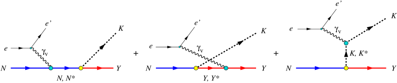
Figure 1: (Color online) The basic Feynman diagrams in the elementary operator.

For the purpose of the nuclear operator, the relativistic elementary operator must be decomposed into its ’non-relativistic’ form. In the case of free Dirac spinors, the operator in Eq. (6) can be decomposed into Pauli space

$$\overline{u}({\mbox{\boldmath${p}$}}_{Y})\,\sum_{i=1}^{6}\,A_{i}M_{i}\,u({\mbox{\boldmath${p}$}}_{N})~{}=~{}N\,\chi_{\rm f}^{\dagger}\,\biggl{[}\,{\cal{F}}_{1}\,{\mbox{\boldmath${\sigma}$}}\cdot{\mbox{\boldmath${\epsilon}$}}+{\cal{F}}_{2}\,{\mbox{\boldmath${\sigma}$}}\cdot{\mbox{\boldmath${k}$}}\,\epsilon_{0}+{\cal{F}}_{3}\,{\mbox{\boldmath${\sigma}$}}\cdot{\mbox{\boldmath${k}$}}\,{\mbox{\boldmath${k}$}}\cdot{\mbox{\boldmath${\epsilon}$}}+{\cal{F}}_{4}\,{\mbox{\boldmath${\sigma}$}}\cdot{\mbox{\boldmath${k}$}}\,{\mbox{\boldmath${p}$}}_{N}\cdot{\mbox{\boldmath${\epsilon}$}}$$ (14)

$$+{\cal{F}}_{5}\,{\mbox{\boldmath${\sigma}$}}\cdot{\mbox{\boldmath${k}$}}\,{\mbox{\boldmath${p}$}}_{Y}\cdot{\mbox{\boldmath${\epsilon}$}}+{\cal{F}}_{6}\,{\mbox{\boldmath${\sigma}$}}\cdot{\mbox{\boldmath${p}$}}_{N}\,\epsilon_{0}+{\cal{F}}_{7}\,{\mbox{\boldmath${\sigma}$}}\cdot{\mbox{\boldmath${p}$}}_{N}\,{\mbox{\boldmath${k}$}}\cdot{\mbox{\boldmath${\epsilon}$}}+{\cal{F}}_{8}\,{\mbox{\boldmath${\sigma}$}}\cdot{\mbox{\boldmath${p}$}}_{N}\,{\mbox{\boldmath${p}$}}_{N}\cdot{\mbox{\boldmath${\epsilon}$}}+{\cal{F}}_{9}\,{\mbox{\boldmath${\sigma}$}}\cdot{\mbox{\boldmath${p}$}}_{N}\,{\mbox{\boldmath${p}$}}_{Y}\cdot{\mbox{\boldmath${\epsilon}$}}$$

$$+{\cal{F}}_{10}\,{\mbox{\boldmath${\sigma}$}}\cdot{\mbox{\boldmath${p}$}}_{Y}\,\epsilon_{0}+{\cal{F}}_{11}\,{\mbox{\boldmath${\sigma}$}}\cdot{\mbox{\boldmath${p}$}}_{Y}\,{\mbox{\boldmath${k}$}}\cdot{\mbox{\boldmath${\epsilon}$}}+{\cal{F}}_{12}\,{\mbox{\boldmath${\sigma}$}}\cdot{\mbox{\boldmath${p}$}}_{Y}\,{\mbox{\boldmath${p}$}}_{N}\cdot{\mbox{\boldmath${\epsilon}$}}+{\cal{F}}_{13}\,{\mbox{\boldmath${\sigma}$}}\cdot{\mbox{\boldmath${p}$}}_{Y}\,{\mbox{\boldmath${p}$}}_{Y}\cdot{\mbox{\boldmath${\epsilon}$}}$$

$$+{\cal{F}}_{14}\,{\mbox{\boldmath${\sigma}$}}\cdot{\mbox{\boldmath${\epsilon}$}}\,{\mbox{\boldmath${\sigma}$}}\cdot{\mbox{\boldmath${k}$}}\,{\mbox{\boldmath${\sigma}$}}\cdot{\mbox{\boldmath${p}$}}_{N}+{\cal{F}}_{15}\,{\mbox{\boldmath${\sigma}$}}\cdot{\mbox{\boldmath${p}$}}_{Y}\,{\mbox{\boldmath${\sigma}$}}\cdot{\mbox{\boldmath${\epsilon}$}}\,{\mbox{\boldmath${\sigma}$}}\cdot{\mbox{\boldmath${k}$}}+{\cal{F}}_{16}\,{\mbox{\boldmath${\sigma}$}}\cdot{\mbox{\boldmath${p}$}}_{Y}\,{\mbox{\boldmath${\sigma}$}}\cdot{\mbox{\boldmath${\epsilon}$}}\,{\mbox{\boldmath${\sigma}$}}\cdot{\mbox{\boldmath${p}$}}_{N}$$

$$+\,{\cal{F}}_{17}\,{\mbox{\boldmath${\sigma}$}}\cdot{\mbox{\boldmath${p}$}}_{Y}\,{\mbox{\boldmath${\sigma}$}}\cdot{\mbox{\boldmath${k}$}}\,{\mbox{\boldmath${\sigma}$}}\cdot{\mbox{\boldmath${p}$}}_{N}\,\epsilon_{0}+{\cal{F}}_{18}\,{\mbox{\boldmath${\sigma}$}}\cdot{\mbox{\boldmath${p}$}}_{Y}\,{\mbox{\boldmath${\sigma}$}}\cdot{\mbox{\boldmath${k}$}}\,{\mbox{\boldmath${\sigma}$}}\cdot{\mbox{\boldmath${p}$}}_{N}\,{\mbox{\boldmath${k}$}}\cdot{\mbox{\boldmath${\epsilon}$}}$$

$$+{\cal{F}}_{19}\,{\mbox{\boldmath${\sigma}$}}\cdot{\mbox{\boldmath${p}$}}_{Y}\,{\mbox{\boldmath${\sigma}$}}\cdot{\mbox{\boldmath${k}$}}\,{\mbox{\boldmath${\sigma}$}}\cdot{\mbox{\boldmath${p}$}}_{N}\,{\mbox{\boldmath${p}$}}_{N}\cdot{\mbox{\boldmath${\epsilon}$}}+\,{\cal{F}}_{20}\,{\mbox{\boldmath${\sigma}$}}\cdot{\mbox{\boldmath${p}$}}_{Y}\,{\mbox{\boldmath${\sigma}$}}\cdot{\mbox{\boldmath${k}$}}\,{\mbox{\boldmath${\sigma}$}}\cdot{\mbox{\boldmath${p}$}}_{N}\,{\mbox{\boldmath${p}$}}_{Y}\cdot{\mbox{\boldmath${\epsilon}$}}\,\biggr{]}\,\chi_{\rm i}~{},$$

where

$$N = \left(\frac{E_{N}+m_{N}}{2m_{N}}\right)^{\frac{1}{2}}\left(\frac{E_{Y}+m_{Y}}{2m_{Y}}\right)^{\frac{1}{2}}~{},$$ (15)

and the individual amplitudes ${\cal F}_{i}$ are given in Appendix A

We will recast the elementary operator to a suitable form for the nuclear process in the next section. As shown in Ref. mart98 the terms of order $p^{2}/m^{2}$, i.e. $F_{16}$–$F_{20}$, can be dropped from the elementary operator, since they come from the small spinor components. Furthermore, this will not disturb the gauge invariance of the operator. Nevertheless, for the sake of accuracy, the omission of these terms should be done carefully. Moreover, unlike the situation in pion production, the particle momenta in our case are always higher than those of pion.

Figure 2: (Color online) Comparison between calculated cross sections obtained by including (solid lines) and excluding (dotted lines) the $D_{13}(1895)$ state with experimental data. Solid squares display the experimental measurement of Niculescu et al. niculescu . This measurement has been reanalyzed by Mohring et al. mohring and shown here by the open circles. The solid diamonds are due to the old measurement by Brauel et al. old_electro . At photon point a photoproduction datum photon_point (open square) is shown for comparison with the transverse cross section.

In this calculation we use the KAON-MAID parameterization kaon-maid . The model consists of gauge-invariant background and resonances terms. The background terms include the standard $s$-, $u$-, and $t$-channel contributions along with a contact term required to restore gauge invariance after hadronic form factors have been introduced Haberzettl:1998eq . The resonance part consists of three nucleon resonances that have been found in the coupled-channels approach to decay into the $K\Lambda$ channel, i.e., the $S_{11}$(1650), $P_{11}$(1710), and $P_{13}(1720)$. Furthermore, the model also includes the $D_{13}(1895)$ state that is found to be important in the description of SAPHIR data saphir .

Figure 3: (Color online) As in Fig. 2, but for photoproduction ($k^{2}=0$). As a comparison, the calculated cross section from Ref. williams is also shown by the dash-dotted line. Solid squares, solid circles represent the experimental data from Refs. Glander:2003jw and Tran:1998qw , respectively. Open squares and open circles represent CLAS Bradford:2005pt and older data old_data , respectively.

At finite $k^{2}$ the calculated transverse and longitudinal cross sections obtained from this model are shown in Fig. 2. Since the model was fitted to the data of Niculescu et al. niculescu , a sizeable discrepancy with the reanalyzed data mohring appears in this figure. However, we note that the model can also nicely describe the old measurement and photoproduction data. As reported in Refs. kaon-maid , the inclusion of the $D_{13}(1895)$ state is important for the description of the structure found in the $\gamma p\to K^{+}\Lambda$ total cross section saphir . We will also investigate the influence of this state in the electroproduction of the hypertriton. To this end we show in Fig. 2 the calculated cross sections when this state were excluded. Obviously, the magnitude of the cross sections is greatly reduced once we omit this state, especially in the case of the longitudinal one, where we can see from Fig. 2 that at $k^{2}=-0.5$ GeV² the cross section is about four times smaller in this case.

In the case of photoproduction, sample of the angular distribution of differential cross section is displayed in Fig. 3, where we compare the prediction of KAON-MAID and that obtained from Ref. williams with experimental data from various measurements. It is obvious from this figure that there exist some discrepancies among the experimental data, especially between the new SAPHIR Glander:2003jw and CLAS Bradford:2005pt data. The discrepancy and its physics consequences have been thoroughly investigated in Ref. Mart:2006dk by means of a multipole model. In spite of this problem, however, Fig. 3 indicates that KAON-MAID still gives a reliable prediction for kaon photoproduction. This becomes more obvious when we compare its prediction with the prediction of Ref. williams , where the latter clearly overestimates the experimental data at the very forward kaon angle. Incidentally, in this region the result of the hypernuclear production is found to be very sensitive to the elementary operator model used Bydzovsky:2006wy .

III The Nuclear Operator and Cross Sections

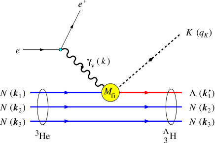
Figure 4: (Color online) Electroproduction of the hypertriton on a ³He target in the impulse approximation, where the virtual photon interacts with only one nucleon inside the ³He. The elementary operator $M_{\rm fi}=\epsilon_{\mu}\,J^{\mu}$ is given in Fig. 1 and Eq. (6).

In analogy to the case of photoproduction mart98 , we write the nuclear transition matrix element in the laboratory frame as (see Fig. 4)

$$\langle\,{\rm f}\left|\,J^{\mu}\,\right|{\rm i}\,\rangle = \sqrt{3}\,\int d^{3}\mbox{\boldmath${p}$}~{}d^{3}\mbox{\boldmath${q}$}~{}\Psi_{\rm f}^{*}(\mbox{\boldmath${p}$},\mbox{\boldmath${q}$}^{\prime})~{}J^{\mu}\,(k^{0},\mbox{\boldmath${k}$},k_{1}^{0},\mbox{\boldmath${k}$}_{1},k_{1}^{\prime 0},\mbox{\boldmath${k}$}_{1}^{\prime},q_{K}^{0},\mbox{\boldmath${q}$}_{K})~{}\Psi_{\rm i}(\mbox{\boldmath${p}$},\mbox{\boldmath${q}$})~{},~{}$$ (16)

where the integrations are taken over the three-body momentum coordinates

$$\mbox{\boldmath${p}$}~{}=~{}\frac{1}{2}\,(\mbox{\boldmath${k}$}_{2}-\mbox{\boldmath${k}$}_{3})~{}~{},~{}~{}\mbox{\boldmath${q}$}~{}=~{}\mbox{\boldmath${k}$}_{1}~{},$$ (17)

and the hyperon momentum in the hypertriton is given by

$$\mbox{\boldmath${q}$}^{\prime} \equiv \mbox{\boldmath${k}$}_{1}^{\prime}~{}=~{}\mbox{\boldmath${k}$}_{1}+\frac{m_{2}+m_{3}}{m_{1}+m_{2}+m_{3}}\,\mbox{\boldmath${Q}$},$$ (18)

with the momentum transfer $\mbox{\boldmath${Q}$}=\mbox{\boldmath${k}$}-\mbox{\boldmath${q}$}_{K}$. The factor of $\sqrt{3}$ on the right hand side of Eq. (16) comes from the anti-symmetry of the initial state. The derivation of this factor is given in Appendix B. Note that in the following we will also use the notations $\mbox{\boldmath${p}$}_{N}\equiv\mbox{\boldmath${k}$}_{1}$ and $\mbox{\boldmath${p}$}_{Y}\equiv\mbox{\boldmath${k}$}_{1}^{\prime}$ in order to facilitate the discussion of the elementary operator.

The ³He wave functions may be written as

$$\Psi_{\rm i}(\mbox{\boldmath${p}$},\mbox{\boldmath${q}$}) = \sum_{\alpha=(LSJljT)}\phi_{\alpha}(p,q)~{}\left|\,\{(LS)J,(l{\textstyle\frac{1}{2}})j\}{\textstyle\frac{1}{2}}M_{\rm i}\ ~{}\right\rangle~{}\left|\,(T{\textstyle\frac{1}{2}}){\textstyle\frac{1}{2}}M_{t}~{}\right\rangle$$ (23)

$$= \sum_{\alpha=(LSJljT)}\sum_{\scriptsize\left.\begin{array}[]{c}\\[-18.08331pt] m_{L}m_{S}m_{l}\\[-6.02777pt] m_{s}m_{J}m_{j}\end{array}\right.}\phi_{\alpha}(p,q)~{}(Lm_{L}Sm_{S}|Jm_{J})~{}(lm_{l}{\textstyle\frac{1}{2}}m_{s}|jm_{j})$$

$$\hskip 85.35826pt\times(Jm_{J}jm_{j}|{\textstyle\frac{1}{2}}M_{\rm i})\,Y^{L}_{m_{L}}(\mbox{\boldmath${\hat{p}}$})Y^{l}_{m_{l}}(\mbox{\boldmath${\hat{q}}$})\chi^{S}_{m_{S}}\chi_{m_{s}}^{\frac{1}{2}}~{}\left|\,(T{\textstyle\frac{1}{2}}){\textstyle\frac{1}{2}}M_{t}~{}\right\rangle~{},$$

where we have used the notation of Ref. deshalit63 for the Clebsch-Gordan coefficients. The hypertriton wave functions can also be written in the form of Eq. (23).

In Eq. (23) we have introduced $\alpha=(LSJljT)$ to shorten the notation, where $L$, $S$, and $T$ are the total angular momentum, spin, and isospin of the pair (2,3), while for particle (1) the corresponding quantum numbers are labeled by $l$, $\frac{1}{2}$, and $\frac{1}{2}$, respectively. Their quantum numbers, along with the probabilities for the 34 partial waves, are listed in Table 1, where we have used the Nijmegen93 version of the ³He wave functions nijmegen93 and the advanced model for the hypertriton wave functions given in Ref. miyagawa93 . Clearly, most contributions will come from the second partial wave ($\alpha=2$), which corresponds to the $S$-wave with isospin 0.

Table 1: Quantum numbers and probabilities (in %) of the ³He and the hypertriton wave functions.

$~{}\alpha~{}$	$~{}L~{}$	$~{}S~{}$	$~{}J~{}$	$~{}l~{}$	$~{}2j~{}$	$~{}2T~{}$	$P(^{3}{\rm He})$	$P(^{3}_{\Lambda}{\rm H})$ miyagawa93
1	0	0	0	0	1	1	44.580	-
2	0	1	1	0	1	0	44.899	93.491
3	2	1	1	0	1	0	2.848	5.794
4	0	1	1	2	3	0	0.960	0.034
5	2	1	1	2	3	0	0.189	0.027
6	1	0	1	1	1	0	0.089	0.004
7	1	0	1	1	3	0	0.198	0.008
8	1	1	0	1	1	1	1.107	-
9	1	1	1	1	1	1	1.113	-
10	1	1	1	1	3	1	0.439	-
11	1	1	2	1	3	1	0.064	-
12	3	1	2	1	3	1	0.306	-
13	1	1	2	3	5	1	1.018	-
14	3	1	2	3	5	1	0.024	-
15	2	0	2	2	3	1	0.274	-
16	2	0	2	2	5	1	0.425	-
17	2	1	2	2	3	0	0.122	0.024
18	2	1	2	2	5	0	0.095	0.018
19	2	1	3	2	5	0	0.205	0.053
20	4	1	3	2	5	0	0.053	0.006
21	2	1	3	4	7	0	0.126	0.010
22	4	1	3	4	7	0	0.038	0.007
23	3	0	3	3	5	0	0.005	0.001
24	3	0	3	3	7	0	0.008	0.001
25	3	1	3	3	5	1	0.051	-
26	3	1	3	3	7	1	0.045	-
27	3	1	4	3	7	1	0.008	-
28	5	1	4	3	7	1	0.074	-
29	3	1	4	5	9	1	0.178	-
30	5	1	4	5	9	1	0.006	-
31	4	0	4	4	7	1	0.053	-
32	4	0	4	4	9	1	0.059	-
33	4	1	4	4	7	0	0.011	0.004
34	4	1	4	4	9	0	0.009	0.003

The elementary operator $J^{\mu}=(J^{0},\mbox{\boldmath${J}$})$ is obtained from Eq. (14), i.e.

$$J^{0} = N~{}\Bigl{\{}\,i{\cal{F}}_{17}\,\mbox{\boldmath${p}$}_{N}\cdot(\mbox{\boldmath${p}$}_{Y}\times\mbox{\boldmath${k}$})+({\cal{F}}_{2}-\mbox{\boldmath${p}$}_{N}\cdot\mbox{\boldmath${p}$}_{Y}\,{\cal{F}}_{17})\,\mbox{\boldmath${\sigma}$}\cdot\mbox{\boldmath${k}$}+({\cal{F}}_{6}+\mbox{\boldmath${p}$}_{Y}\cdot\mbox{\boldmath${k}$}\,{\cal{F}}_{17})\,\mbox{\boldmath${\sigma}$}\cdot\mbox{\boldmath${p}$}_{N}$$ (24)

$$\hskip 19.91692pt+\,({\cal{F}}_{10}+\mbox{\boldmath${p}$}_{N}\cdot\mbox{\boldmath${k}$}\,{\cal{F}}_{17})\,\mbox{\boldmath${\sigma}$}\cdot\mbox{\boldmath${p}$}_{Y}\Bigr{\}}~{},$$

and

$${J} = -N~{}\Bigl{[}~{}({\cal{F}}_{1}+{\cal{F}}_{14}\;\mbox{\boldmath${p}$}_{N}\cdot\mbox{\boldmath${k}$}-{\cal{F}}_{15}\;\mbox{\boldmath${p}$}_{Y}\cdot\mbox{\boldmath${k}$}-{\cal{F}}_{16}\;\mbox{\boldmath${p}$}_{N}\cdot\mbox{\boldmath${p}$}_{Y})~{}\mbox{\boldmath${\sigma}$}$$ (25)

$$\hskip 19.91692pt+~{}\mbox{\boldmath${\sigma}$}\cdot\mbox{\boldmath${k}$}~{}~{}~{}\{~{}({\cal{F}}_{3}-\mbox{\boldmath${p}$}_{N}\cdot\mbox{\boldmath${p}$}_{Y}\;{\cal{F}}_{18})\;\mbox{\boldmath${k}$}+({\cal{F}}_{4}-{\cal{F}}_{14}-\mbox{\boldmath${p}$}_{N}\cdot\mbox{\boldmath${p}$}_{Y}\;{\cal{F}}_{19})\;\mbox{\boldmath${p}$}_{N}$$

$$\hskip 62.59605pt+~{}({\cal{F}}_{5}+{\cal{F}}_{15}-\mbox{\boldmath${p}$}_{N}\cdot\mbox{\boldmath${p}$}_{Y}\;{\cal{F}}_{20})\;\mbox{\boldmath${p}$}_{Y}~{}\}$$

$$\hskip 19.91692pt+~{}\mbox{\boldmath${\sigma}$}\cdot\mbox{\boldmath${p}$}_{N}\,\{~{}({\cal{F}}_{7}+{\cal F}_{14}+\mbox{\boldmath${p}$}_{Y}\cdot\mbox{\boldmath${k}$}\;{\cal{F}}_{18})\;\mbox{\boldmath${k}$}+({\cal{F}}_{8}+\mbox{\boldmath${p}$}_{Y}\cdot\mbox{\boldmath${k}$}\;{\cal{F}}_{19})\;\mbox{\boldmath${p}$}_{N}$$

$$\hskip 62.59605pt+~{}({\cal{F}}_{9}+{\cal{F}}_{16}+\mbox{\boldmath${p}$}_{Y}\cdot\mbox{\boldmath${k}$}\;{\cal{F}}_{20})\;\mbox{\boldmath${p}$}_{Y}~{}\}$$

$$\hskip 19.91692pt+~{}\mbox{\boldmath${\sigma}$}\cdot\mbox{\boldmath${p}$}_{Y}\,\{~{}({\cal{F}}_{11}+{\cal F}_{15}+\mbox{\boldmath${p}$}_{N}\cdot\mbox{\boldmath${k}$}\;{\cal{F}}_{18})\;\mbox{\boldmath${k}$}+~{}({\cal{F}}_{12}+{\cal F}_{16}+\mbox{\boldmath${p}$}_{N}\cdot\mbox{\boldmath${k}$}\;{\cal{F}}_{19})\;\mbox{\boldmath${p}$}_{N}$$

$$\hskip 62.59605pt+~{}({\cal{F}}_{13}+\mbox{\boldmath${p}$}_{N}\cdot\mbox{\boldmath${k}$}\;{\cal{F}}_{20})\;\mbox{\boldmath${p}$}_{Y}~{}\}$$

$$\hskip 19.91692pt+~{}i\;\{-{\cal{F}}_{14}\;\mbox{\boldmath${p}$}_{N}\times\mbox{\boldmath${k}$}-{\cal{F}}_{15}\;\mbox{\boldmath${p}$}_{Y}\times\mbox{\boldmath${k}$}+{\cal{F}}_{16}\,\mbox{\boldmath${p}$}_{N}\times\mbox{\boldmath${p}$}_{Y}$$

$$\hskip 48.36967pt+~{}\mbox{\boldmath${p}$}_{N}\cdot(\mbox{\boldmath${p}$}_{Y}\times\mbox{\boldmath${k}$})\;({\cal{F}}_{18}\;\mbox{\boldmath${k}$}+{\cal{F}}_{19}\;\mbox{\boldmath${p}$}_{N}+{\cal{F}}_{20}\;\mbox{\boldmath${p}$}_{Y}\,)~{}\}~{}\Bigr{]}~{}.$$

It is obvious from Eqs. (8)–(13) that the gauge invariance of the elementary operator relates Eq. (24) and Eq. (25) by

$$J_{0} = \mbox{\boldmath${k}$}\cdot\mbox{\boldmath${J}$}\,/\,k_{0}~{},$$ (26)

which slightly simplifies the numerical calculation since we can eliminate either $J^{0}$ or $J_{z}$ by $\mbox{\boldmath${k}$}\cdot\mbox{\boldmath${J}$}=|\mbox{\boldmath${k}$}|J_{z}$.

For the purpose of calculating the observables it is useful to rewrite the elementary operator in the form of a matrix $[j]$, through the relation $J^{\mu}=[\sigma]\,[j]$, i.e.,

$$J^{\mu} = (1,\sigma_{x},\sigma_{y},\sigma_{z})\left(\begin{array}[]{cccc}j_{00}&j_{x0}&j_{y0}&j_{z0}\\ j_{0x}&j_{xx}&j_{yx}&j_{zx}\\ j_{0y}&j_{xy}&j_{yy}&j_{zy}\\ j_{0z}&j_{xz}&j_{yz}&j_{zz}\end{array}\right)~{},$$ (31)

where the individual components are given in Appendix C.

Since the hypertriton has isospin 0, we may drop the isospin part of the wave functions. By inserting the two nuclear wave functions in Eq. (16) and writing symbolically ${\sf m}=(m_{L}m_{S}m_{l}m_{s}m_{J}m_{j})$ for the sake of brevity, we can recast the transition matrix element in the form of

$$\langle\,{\rm f}\left|\,J^{\mu}\,\right|{\rm i}\,\rangle = \sqrt{3}\,\sum_{\alpha,\alpha^{\prime}}\sum_{{\sf mm}^{\prime}}\left(Lm_{L}Sm_{S}|Jm_{J}\right)\,\left(Lm_{L}Sm_{S}|J^{\prime}m_{J^{\prime}}\right)\,\left(lm_{l}{\textstyle\frac{1}{2}}m_{s}|jm_{j}\right)$$ (32)

$$\times\,\left(l^{\prime}m_{l^{\prime}}{\textstyle\frac{1}{2}}m_{s^{\prime}}|j^{\prime}m_{j^{\prime}}\right)\,\left(Jm_{J}jm_{j}|{\textstyle\frac{1}{2}}M_{\rm i}\right)\,\left(J^{\prime}m_{J^{\prime}}j^{\prime}m_{j^{\prime}}|{\textstyle\frac{1}{2}}M_{\rm f}\right)$$

$$\times\,\delta_{LL^{\prime}}\,\delta_{m_{L}m_{L^{\prime}}}\,\delta_{SS^{\prime}}\,\delta_{m_{S}m_{S^{\prime}}}\,\delta_{T0}$$

$$\times\,\int p^{2}dp~{}d^{3}\mbox{\boldmath${q}$}\;\phi_{\alpha^{\prime}}(p,q^{\prime})\;\phi_{\alpha}(p,q)\;Y^{l^{\prime}}_{m_{l^{\prime}}}(\mbox{\boldmath${\hat{q}}$}^{\prime})\,Y^{l}_{m_{l}}(\mbox{\boldmath${\hat{q}}$})\;\langle{\textstyle\frac{1}{2}},m_{s^{\prime}}\,|\,J^{\mu}\,|\,{\textstyle\frac{1}{2}},m_{s}\rangle\,,$$

where we have performed the integration over the spectator solid angle,

$$\int d\hat{\mbox{\boldmath${p}$}}~{}Y^{L^{\prime}*}_{m_{L^{\prime}}}(\hat{\mbox{\boldmath${p}$}})\,Y^{L}_{m_{L}}(\hat{\mbox{\boldmath${p}$}}) = \delta_{LL^{\prime}}\,\delta_{m_{L}m_{L^{\prime}}}~{},$$ (33)

as the relative momentum of the two spectators ${p}$ does not change. By using

$$J^{\mu} = j^{\mu}_{0}+\sigma_{x}\,j^{\mu}_{x}+\sigma_{y}\,j^{\mu}_{y}+\sigma_{z}\,j^{\mu}_{z}$$ (34)

$$= \sum_{n=0,1}\;\sum_{m_{n}=-n}^{+n}\,(-1)^{m_{n}}\,\sigma^{(n)}_{-m_{n}}\,[\,j^{\mu}\,]^{(n)}_{m_{n}}~{},$$

where the components of $[\,j^{\mu}\,]^{(n)}_{m_{n}}$ are given in Eq. (31) and Appendix C, with

$$\left[\,j^{\mu}\,\right]^{(0)} = j^{\mu}_{0}~{},$$ (35)

$$\left[\,j^{\mu}\,\right]^{(1)}_{\pm 1} = \mp\frac{1}{\sqrt{2}}(j^{\mu}_{x}\pm ij^{\mu}_{y})~{},$$ (36)

$$\left[\,j^{\mu}\,\right]^{(1)}_{0} = j^{\mu}_{z}~{},$$ (37)

$$\sigma^{(0)} = 1~{},$$ (38)

$$\sigma^{(1)} = \mbox{\boldmath${\sigma}$}~{},$$ (39)

and

$$\langle{\textstyle\frac{1}{2}},m_{s^{\prime}}\,|\,\sigma_{-m_{n}}^{(n)}\,|\,{\textstyle\frac{1}{2}},m_{s}\rangle = \sqrt{2}\,(-1)^{n-\frac{1}{2}-m_{s^{\prime}}+m_{n}}\left({\textstyle\frac{1}{2}}-\!m_{s^{\prime}}{\textstyle\frac{1}{2}}m_{s}|nm_{n}\right)~{},$$ (40)

we can rewrite Eq. (32) in the form of

$$\langle\,{\rm f}\left|\,J^{\mu}\,\right|{\rm i}\,\rangle = \sqrt{6}\,\sum_{\alpha,\alpha^{\prime}}~{}\sum_{{\sf m},{\sf m}^{\prime}}~{}\sum_{n,m_{n}}\left(Lm_{L}Sm_{S}|Jm_{J}\right)\,\left(Lm_{L}Sm_{S}|J^{\prime}m_{J^{\prime}}\right)\,\left(lm_{l}{\textstyle\frac{1}{2}}m_{s}|jm_{j}\right)$$ (41)

$$\times\,\left(l^{\prime}m_{l^{\prime}}{\textstyle\frac{1}{2}}m_{s^{\prime}}|j^{\prime}m_{j^{\prime}}\right)\,\left(Jm_{J}jm_{j}|{\textstyle\frac{1}{2}}M_{\rm i}\right)\,\left(J^{\prime}m_{J^{\prime}}j^{\prime}m_{j^{\prime}}|{\textstyle\frac{1}{2}}M_{\rm f}\right)\,\left({\textstyle\frac{1}{2}}-\!m_{s^{\prime}}{\textstyle\frac{1}{2}}m_{s}|nm_{n}\right)$$

$$\times\,(-1)^{n-\frac{1}{2}-m_{s^{\prime}}}\delta_{LL^{\prime}}\,\delta_{m_{L}m_{L^{\prime}}}\,\delta_{SS^{\prime}}\,\delta_{m_{S}m_{S^{\prime}}}\,\delta_{T0}$$

$$\times\,\int p^{2}dp~{}d^{3}\mbox{\boldmath${q}$}\;\phi_{\alpha^{\prime}}(p,q^{\prime})\;\phi_{\alpha}(p,q)\;Y^{l^{\prime}}_{m_{l^{\prime}}}(\mbox{\boldmath${\hat{q}}$}^{\prime})\,Y^{l}_{m_{l}}(\mbox{\boldmath${\hat{q}}$})\;\left[\,j^{\mu}\,\right]^{(n)}_{m_{n}}\,.$$

Note that the elementary operator $\left[\,j^{\mu}\,\right]^{(n)}_{m_{n}}$ is completely frame independent, since it is independent from the frame where $\epsilon^{\mu}$ and $\sigma^{(n)}$ are defined. Hence, by summing and averaging over the nuclear spins we can construct the spin averaged Lorentz tensor tiator81

$$W^{\mu\nu} = \frac{1}{2}\sum_{M_{\rm i}M_{\rm f}}\langle\,{\rm f}\left|\,J^{\mu}\,\right|{\rm i}\,\rangle\langle\,{\rm f}\left|\,J^{\nu}\,\right|{\rm i}\,\rangle^{*}~{},$$ (42)

which is related to the nuclear structure functions by

$$W_{\rm T} = \frac{1}{4\pi}~{}(W_{xx}+W_{yy})~{},$$ (43)

$$W_{\rm L} = \frac{1}{4\pi}~{}W_{00}~{},$$ (44)

$$W_{\rm TT} = \frac{1}{4\pi}~{}(W_{xx}-W_{yy})~{},$$ (45)

$$W_{\rm LT} = \frac{1}{4\pi}~{}(W_{0x}+W_{x0})~{}.$$ (46)

The exclusive cross section ${}^{3}{\rm He}(e,e^{\prime}K^{+})^{3}_{\Lambda}{\rm H}$ can be written as

$$\frac{d^{5}\sigma}{d\varepsilon_{\rm f}\,d\Omega_{e^{\prime}}\,d\Omega_{K}} = \Gamma~{}\frac{d\sigma_{v}}{d\Omega_{K}}~{},$$ (47)

where the flux of virtual photons is given by

$$\Gamma = \frac{\alpha}{2\pi^{2}}~{}\frac{\varepsilon_{\rm f}}{\varepsilon_{\rm i}}~{}K_{L}~{}\frac{1}{-k^{2}}~{}\frac{1}{1-\epsilon}~{},$$ (48)

and the differential cross section for kaons produced by virtual photons can be written as

$$\frac{d\sigma_{v}}{d\Omega_{K}} = \frac{d\sigma_{\rm T}}{d\Omega_{K}}+\epsilon_{\rm L}~{}\frac{d\sigma_{\rm L}}{d\Omega_{K}}+\epsilon~{}\frac{d\sigma_{\rm TT}}{d\Omega_{K}}~{}\cos 2\phi_{K}+\sqrt{2\epsilon_{\rm L}(1+\epsilon)}~{}\frac{d\sigma_{\rm LT}}{d\Omega_{K}}~{}\cos\phi_{K}~{},$$ (49)

with the virtual photon polarization of

$$\epsilon = \left(1-2\,\frac{\mbox{\boldmath${k}$}^{2}}{k^{2}}\,\tan^{2}{\textstyle\frac{1}{2}}\theta_{e}\right)^{-1}~{},$$ (50)

and

$$\epsilon_{\rm L} = -\frac{k^{2}}{\mbox{\boldmath${k}$}^{2}}\,\epsilon~{}.$$ (51)

The cross sections are conventionally measured in the c.m. system. In this frame of reference the individual cross sections are given by

$$\frac{d\sigma_{\rm T}}{d\Omega_{K}^{\rm c.m.}} = \alpha_{e}\,\frac{q_{K}^{\rm c.m.}}{K_{L}}\,\frac{M_{{}^{3}_{\Lambda}\!{\rm H}}}{2W}\,W_{\rm T}^{\rm c.m.}~{},$$ (52)

$$\frac{d\sigma_{\rm L}}{d\Omega_{K}^{\rm c.m.}} = \alpha_{e}\,\frac{q_{K}^{\rm c.m.}}{K_{L}}\,\frac{M_{{}^{3}_{\Lambda}\!{\rm H}}}{W}\,W_{\rm L}^{\rm c.m.}~{},$$ (53)

$$\frac{d\sigma_{\rm TT}}{d\Omega_{K}^{\rm c.m.}} = \alpha_{e}\,\frac{q_{K}^{\rm c.m.}}{K_{L}}\,\frac{M_{{}^{3}_{\Lambda}\!{\rm H}}}{2W}\,W_{\rm TT}^{\rm c.m.}~{},$$ (54)

$$\frac{d\sigma_{\rm LT}}{d\Omega_{K}^{\rm c.m.}} = -\alpha_{e}\,\frac{q_{K}^{\rm c.m.}}{K_{L}}\,\frac{M_{{}^{3}_{\Lambda}\!{\rm H}}}{2W}\,W_{\rm LT}^{\rm c.m.}~{},$$ (55)

where $\alpha_{e}=e^{2}/4\pi$ the fine structure constants and we have defined the photon equivalent energy [also in Eq. (48)]

$$K_{L} = \frac{W^{2}-M_{\rm He}^{2}}{2M_{\rm He}}~{}.$$ (56)

The transformation from the laboratory to c.m. frames affects the longitudinal structure functions only and leaves the transverse ones unchanged, i.e.,

$$W_{\rm T}^{\rm c.m.} = W_{\rm T}^{\rm lab}~{},$$ (57)

$$W_{\rm L}^{\rm c.m.} = W_{\rm L}^{\rm lab}\,{\mbox{\boldmath${k}$}_{\rm c.m.}^{2}}/{\mbox{\boldmath${k}$}^{2}}~{},$$ (58)

$$W_{\rm TT}^{\rm c.m.} = W_{\rm TT}^{\rm lab}~{},$$ (59)

$$W_{\rm LT}^{\rm c.m.} = W_{\rm LT}^{\rm lab}\,\sqrt{{\mbox{\boldmath${k}$}_{\rm c.m.}^{2}}/{\mbox{\boldmath${k}$}^{2}}}~{}.$$ (60)

IV Results and Discussion

The summations over ${\sf m}$ and ${\sf m}^{\prime}$ in Eq. (41) are significantly reduced by the properties of the Clebsch-Gordan coefficient. As the result, we only need to sum over the angular-momentum and spin projections $m_{J},m_{J^{\prime}},m_{S}$, and $m_{s}$, since the other projections are fixed by the relations

$$m_{s^{\prime}} = m_{s}-m_{n}~{},$$ (61)

$$m_{j^{\prime}} = M_{\rm f}-m_{J^{\prime}}~{},$$ (62)

$$m_{j} = M_{\rm i}-m_{J}~{},$$ (63)

$$m_{L} = m_{J^{\prime}}-m_{S}~{},$$ (64)

$$m_{l^{\prime}} = m_{j^{\prime}}-m_{s^{\prime}}~{},$$ (65)

$$m_{l} = m_{j}-m_{s}~{}.$$ (66)

As the first step, we need to check our Fortran code. This has been performed by calculating the elementary cross sections and comparing the results with those obtained from the original elementary code. For this purpose we replace the wave functions in Eq. (41) by unity. As a consequence, Eq. (41) is greatly reduced to

$$\langle\,{\rm f}\left|\,J^{\mu}\,\right|{\rm i}\,\rangle = \sqrt{2}\,\sum_{n,m_{n}}(-1)^{n-1/2-M_{\rm f}}\left({\textstyle\frac{1}{2}}\;-\!\!M_{\rm f}\;{\textstyle\frac{1}{2}}\;M_{\rm i}|nm_{n}\right)\,\left[\,j^{\mu}\,\right]^{(n)}_{m_{n}}\,,$$ (67)

and the transverse and longitudinal cross sections can expressed in terms of

$$\frac{d\sigma_{\rm T}}{d\Omega_{K}^{\rm c.m.}} = \frac{q_{K}^{\rm c.m.}}{k^{\rm c.m.}}\,\frac{m_{p}m_{\Lambda}}{32\pi^{2}W^{2}}\,\sum_{i=0}^{3}\left(|j_{ix}|^{2}+|j_{iy}|^{2}\right)~{},$$ (68)

$$\frac{d\sigma_{\rm L}}{d\Omega_{K}^{\rm c.m.}} = \frac{q_{K}^{\rm c.m.}}{k^{\rm c.m.}}\,\frac{m_{p}m_{\Lambda}}{32\pi^{2}W^{2}}\,\sum_{i=0}^{3}2|j_{i0}|^{2}~{},$$ (69)

which can be shown to be identical with the standard definitions of the transverse and longitudinal cross sections in the elementary process. However, we do not use Eqs. (68) and (69) to check the code. Instead, we calculate the elementary cross sections by using the main code, that is used to compute the nuclear cross sections, but we replace the wave functions in Eq. (41) by unity. The output of the Fortran code shows a precise agreement with the cross sections calculated directly by using the CGLN amplitudes chew (i.e. the solid lines in Figs. 2 and 3), which is the standard way of calculating the cross sections in KAON-MAID. This result convinces us that our code has calculated the cross sections properly.

IV.1 Photoproduction of the Hypertriton

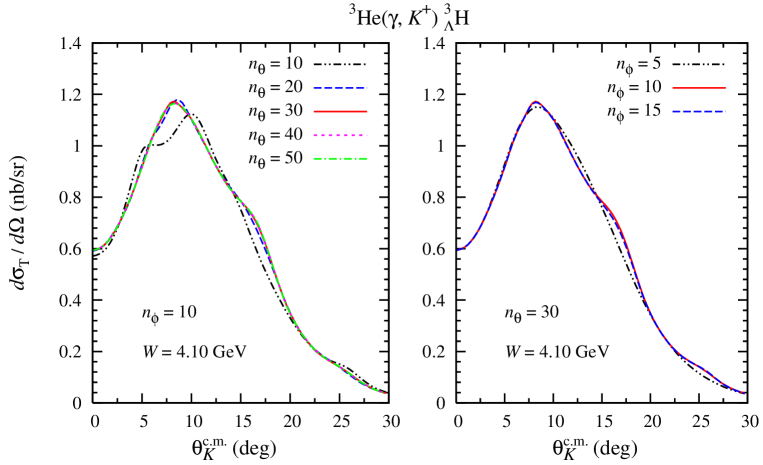
Figure 5: (Color online) Variations of the hypertriton photoproduction cross section for different values of the number of Gauss supporting points $n_{\theta}$ and $n_{\phi}$ in the angular integration of $d{\mbox{\boldmath${\hat{q}}$}}$. Only $s$-wave parts of the nuclear wave functions have been used to obtain these curves.

As shown in Table 1 the initial ³He wave function contains 34 components and the final hypertriton wave function contains 16 components. Since we use the impulse approximation, the quantum numbers of the pair remain unchanged, which is represented by the three Kronecker delta functions $\delta_{LL^{\prime}}\delta_{SS^{\prime}}\delta_{T0}$ in Eq. (41). This selection rule significantly reduces the number of non-zero diagonal and interference terms for the components of wave functions from $34\times 16$ to just 64 components. In both wave functions the number of supporting points for the $p$ and $q$ momenta are 34 and 20, respectively.

To calculate the four-dimensional integrals in Eq. (41) we have used Gaussian integration. We first carried out the overlap integral in $p$, because it is easier, and stored the result in a $20\times 20\times 64$ array, where the last component is intended for the index of the non-zero overlap integrals. Since the computation of the integrals is very time consuming, the number of the supporting points should be limited as small as possible, without sacrifying the numerical stability of the integration. To this end in Fig. 5 we display the variations of the cross sections as functions of the number of Gauss supporting points for the angular integration in Eq. (41), i.e., $n_{\theta}$ and $n_{\phi}$. It is obvious from this figure that the result of integrations starts to become stable for $n_{\theta}\geq 30$ and $n_{\phi}\geq 10$. Therefore, in the following discussion we shall only use the results with $n_{\theta}=30$ and $n_{\phi}=10$. For the full calculation at every point of cross sections of interest we have carried out an integration over $34\times 20\times 64\times 30\times 10=13056000$ grid points. The numerical computation becomes more challenging because the integrand consists of the elementary operator $\left[\,j^{\mu}\,\right]^{(n)}_{m_{n}}$ in the form of $4\times 4$ complex-component matrix. Fortunately, current conservation given by Eq. (26) reduces the required information to $4\times 3=12$ components. The result, which is equivalent to an integration over 156 millions grid points, is then summed over angular momentum and spin projections $m_{J},m_{J^{\prime}},m_{S}$, and $m_{s}$, as described above.

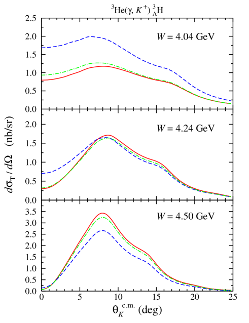
Figure 6: (Color online) Effects of Fermi motion on the differential cross sections at three different total c.m. energies. The dashed curve is obtained from the “frozen nucleon” approximation ($\langle{\mbox{\boldmath${k}$}}_{1}\rangle=0$), the dash-dotted curve is obtained with an average momentum of $\langle{\mbox{\boldmath${k}$}}_{1}\rangle=-\frac{1}{3}{\mbox{\boldmath${Q}$}}$, while the solid curve shows the exact treatment of Fermi motion.

As in the previous study mart98 we have also investigated contribution of non-localities generated by Fermi motion in the initial and final nuclei. The exact treatment of Fermi motion is included in the integrations over the wave functions in Eq. (41), whereas a local approximation can be carried out by freezing the operator at an average nucleon momentum

$$\langle{\mbox{\boldmath${k}$}}_{1}\rangle = -\kappa\frac{A-1}{2A}{\mbox{\boldmath${Q}$}}~{}=~{}-\frac{\kappa}{3}\mbox{\boldmath${Q}$}~{},$$ (70)

since $A=3$. For $\kappa=0$, Eq. (70) corresponds to the “frozen nucleon” approximation, whereas $\kappa=1$ yields the average momentum approximation.

Figure 6 displays the effect of Fermi motion on the differential cross sections at three different total c.m. energies. Note that these energies correspond to the photon lab energies $E_{\gamma}=1.5$ GeV, 1.8 GeV, and 2.2 GeV, used in our previous work mart98 for making the comparison easier. Reference tiator2 has shown that the effect of Fermi motion in the pion photoproduction in the $s$- and $p$-shells is in part simulated by the average momentum assumption $\langle{\mbox{\boldmath${k}$}}_{1}\rangle=-\frac{1}{3}{\mbox{\boldmath${Q}$}}$. Figure 6 obviously shows that this phenomenon is also found in the hypertriton photoproduction, whereas the use of “frozen nucleon” approximation ($\langle{\mbox{\boldmath${k}$}}_{1}\rangle=0$) leads to significantly different results. Although the average momentum assumption can approximate the exact treatment of Fermi motion, for the sake of accuracy we will use the exact treatment of Fermi motion in the following discussion.

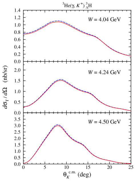
Figure 7: (Color online) The effect of the Coulomb correction on the differential cross sections at three different total c.m. energies. The dashed curves show the results without Coulomb correction, whereas the solid lines are obtained after including this correction.

In the final state the positively charged kaon interacts with the hypertriton by means of the Coulomb force. Therefore, in our calculation a Coulomb correction factor must be taken into account. For this purpose we follow Ref. tia_th , who introduced the Gamow factor

$$F_{G}(|\mbox{\boldmath${q}$}_{K}|) = \frac{2\pi\zeta}{{\rm exp}[2\pi\zeta]-1}~{},$$ (71)

with

$$\zeta = \frac{\alpha_{e}}{v_{K}}~{}=~{}\alpha_{e}~{}\frac{E_{K}}{|\mbox{\boldmath${q}$}_{K}|}~{},$$ (72)

and $\alpha_{e}=e^{2}/4\pi$ to account for the Coulomb effect in pion photoproduction off ³He at threshold. In Ref. tia_th it has been shown that this factor is important to help to describe experimental data at threshold. In the case of hypertriton production this factor is found to be negligible, as shown in Fig. 7. The same finding has been also reported by the previous study mart98 . This result can be understood, because the corresponding photon energy in the present work (as well as in Ref mart98 ) is much higher than the threshold energy of pion photoproduction on ³He.

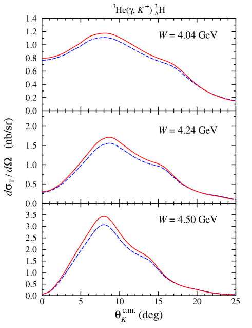
Figure 8: (Color online) Effects of the higher partial waves in the ${}^{3}{\rm He}(\gamma,K^{+})^{3}_{\Lambda}{\rm H}$ process at three different total c.m. energies. Dashed curves are the cross sections obtained by using only $s$-wave, while solid curves exhibit the results after including all partial waves listed in Table 1.

The influence of higher partial waves on the cross section is shown in Fig. 8. As shown in this figure the effect is only essential at the cross section bumps ($\theta_{K}^{\rm c.m.}\approx 8^{\circ}$), while at very small (and very large) kaon scattering angle the effect vanishes. Nevertheless, for the sake of accuracy, the following results have been obtained from calculations by using all available partial waves given in Table 1.

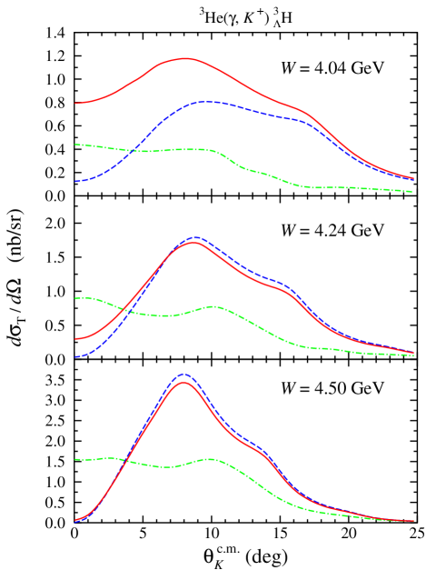
Figure 9: (Color online) Comparison between differential cross sections of hypertriton photoproduction obtained in the present work with the missing resonance $D_{13}(1895)$ included in the elementary operator (solid lines) and those obtained by excluding this resonance (dashed lines). Results from the previous work mart98 which have been obtained by using different nuclear wave functions and different elementary operator williams are shown by the dash-dotted lines. In all cases all available partial waves have been taken into account.

As in the elementary process, contribution of the missing resonance $D_{13}(1895)$ in the hypertriton production is also found to be significant, especially at $W=4.04$ GeV (see Fig. 9). We feel that this is reasonable, because the energy corresponds to the elementary total c.m. energy $W_{\gamma p\to K\Lambda}=1.9$ GeV, i.e., almost at the resonance pole position. As shown in Fig. 9, the effect gradually disappears at higher energies. We note that, due to the strong nuclear suppression at large kaon scattering angles, this effect also vanishes for $\theta_{K}^{\rm c.m.}>25^{\circ}$. Therefore, $W\approx 4.04$ and $0^{\circ}\lesssim\theta_{K}^{\rm c.m.}\lesssim 20^{\circ}$ represent an example of the recommended kinematics for the measurement of hypertriton photoproduction. This conclusion is apparently also supported by Fig. 6, where for this kinematics the variation of differential cross sections due to the effect of non-localities is found to be remarkable.

From Fig. 9 we also observe that the present calculation yields considerable discrepancy with the result of the previous calculation mart98 . We estimate that this discrepancy originates from the different nuclear wave functions and elementary operator used. Previous calculation mart98 used the wave function of ³He obtained as a solution of the Faddeev equations with the Reid soft core potential kim , and the simple hypertriton wave function developed in Ref. congleton that consists of only two partial waves. Furthermore, we note that in Ref. mart98 the calculated differential cross section would increase by a factor of about three if only $s$-wave were used (see Fig. 5 of Ref. mart98 ), in spite of the fact that contribution from other partial waves is less than 6% (see Table I of Ref. mart98 ). In conclusion we would like to say that present calculation provides a more reliable result, since it uses more accurate nuclear wave functions nijmegen93 ; miyagawa93 and elementary operator kaon-maid , while the effect of the high-momentum partial waves seems to be more reasonable.

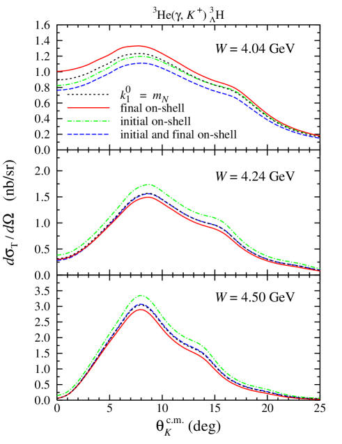
Figure 10: (Color online) The effect of different off-shell assumptions on the differential cross section calculated at three different total c.m. energies. The dash-dotted curves illustrate the calculation with the initial nucleon in ³He on-shell, i.e., $\left[k_{1}^{0}=(m_{N}^{2}+{\mbox{\boldmath${k}$}}_{1}^{2})^{1/2}\right]$, while solid curves are obtained by assuming the final hyperon in the hypertriton to be on-shell $\left[k_{1}^{\prime 0}=(m_{Y}^{2}+{\mbox{\boldmath${k}$}}_{1}^{\prime 2})^{1/2}\right]$. The dashed curves show the calculation with both initial and final baryons are on-shell, while the dotted curves are obtained by assuming $k_{1}^{0}=m_{N}$ (both initial and final baryons are off-shell).

It is obvious that all baryons involved in the hypertriton productions are off-shell. The elementary operator has been, however, constructed and fitted to experimental data where both initial nucleon and final hyperon are on-shell. In view of this, it is of interest to study the influence of the off-shell behavior of these baryons on the calculated cross sections. For this purpose we make four assumptions:

1. Both initial and final baryons are on-shell,

   $$k_{1}^{0}=(m_{N}^{2}+{\mbox{\boldmath${k}$}}_{1}^{2})^{1/2}~{}~{}~{},~{}~{}~{}k_{1}^{\prime 0}=(m_{Y}^{2}+{\mbox{\boldmath${k}$}}_{1}^{\prime 2})^{1/2}~{}.$$ (73)

2. The initial nucleon is on-shell and the final hyperon is off-shell,

   $$k_{1}^{0}=(m_{N}^{2}+{\mbox{\boldmath${k}$}}_{1}^{2})^{1/2}~{}~{}~{},~{}~{}~{}k_{1}^{\prime 0}=k_{1}^{0}+k_{0}-E_{K}~{}.$$ (74)

3. The initial nucleon is off-shell and the final hyperon is on-shell,

   $$k_{1}^{0}=k_{1}^{\prime 0}+E_{K}-k_{0}~{}~{}~{},~{}~{}~{}k_{1}^{\prime 0}=(m_{Y}^{2}+{\mbox{\boldmath${k}$}}_{1}^{\prime 2})^{1/2}~{}.$$ (75)

4. Both initial and final baryons are off-shell. In this case the static approximation,

   $$k_{1}^{0}=m_{N}~{}~{}~{},~{}~{}~{}k_{1}^{\prime 0}=k_{1}^{0}+k_{0}-E_{K}~{},$$ (76)

   is used.

Note that we have used the first assumption in the previous figures for the sake of simplicity. These four different off-shell assumptions result in complicated variations of the differential cross sections as depicted in Fig. 10. At $W=4.04$ GeV the first assumption yields the smallest cross section, while the third assumption leads to the largest cross section. However, at higher $W$ the situation changes, the latter gives in fact the smallest cross sections. At $W=4.04$ GeV we estimate that experimental data at forward angles with about 10% error bars would be able to check these off-shell assumptions. For other kinematics (higher $W$) the cross section differences are presumably to small in view of the present technology Dohrmann:2004xy .

IV.2 Electroproduction of the Hypertriton

It has been widely known that electroproduction process offers more possibilities to study the structure of nucleons and nuclei. Furthermore, Ref. tiator81 , e.g., has shown that electroproduction of pion off ³He reveals different phenomena, compared to photoproduction of pion on ³He. The effects of Fermi motion, for instance, is found to be more profound in electroproduction rather than in photoproduction. The effects of different off-shell assumptions are also found to be more considerable in electroproduction, especially in the transverse cross section. Motivated by these observations, here we continue our investigation described in Subsection IV.1 to the finite $k^{2}$ regions.

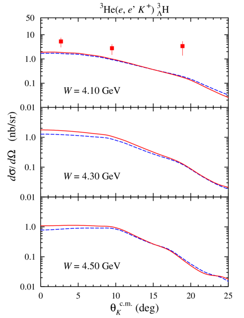
Figure 11: (Color online) The effect of the $s$-wave approximation on the differential cross section of the hypertriton electroproduction. The dashed curves are the cross sections obtained by using only $s$-wave, while the solid curves exhibit the results after including all partial waves listed in Table 1. The curves have been obtained from Eq. (49) with $k^{2}=-0.35$ GeV² and $\epsilon=0.762$, whereas the azimuth angle $\phi$ has been averaged. Experimental data are from Ref. Dohrmann:2004xy .

The result for hypertriton electroproduction shows, however, different behavior compared to the case of pion electroproduction of ³He. This is demonstrated by Fig. 11, where we can see that the effect of the higher partial waves is considerably smaller than in the case of photoproduction (cf. Fig. 8). Only at higher $W$ and very forward directions, where the momentum transfer ${Q}$ is significantly large, the effects are sizable. Note that the electroproduction cross sections exhibit quite different shapes compared to the photoproduction ones. This indicates that the longitudinal terms dominate other contributions in all three kinematics shown in Fig. 11. This conjecture is proven by Fig. 12, from which it is obvious that the fall-off structure of the longitudinal cross sections drives the whole shapes of the cross section shown in Fig. 11, whereas the behavior of the transverse cross sections (with peaks at $\theta_{K}^{\rm c.m.}\approx 8^{\circ}$) is similar to that of the photoproduction cross sections given in Fig. 8.

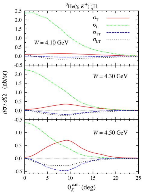
Figure 12: (Color online) Individual differential cross sections, $d\sigma_{\rm T}/d\Omega$, $d\sigma_{\rm L}/d\Omega$, $d\sigma_{\rm TT}/d\Omega$, and $d\sigma_{\rm LT}/d\Omega$, as a function of the kaon scattering angle at three different total c.m. energies.

We have found that the dominant behavior of the longitudinal cross sections originate from the missing resonance $D_{13}(1895)$. Excluding this resonance results in a reduction of the longitudinal cross sections by one order of magnitude, whereas the transverse ones decreases only by a factor of two. This result indicates that the behavior of the longitudinal terms in the elementary operator (see Fig. 2) is persistent and even gets amplified in the nuclear cross sections.

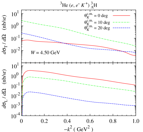
Figure 13: (Color online) Transverse and longitudinal cross sections as a function of the virtual photon momentum squared at three different kaon scattering angles.

The $k^{2}$ evolutions of both transverse and longitudinal cross sections are displayed in Fig. 13. Both Figs. 12 and 13 reveals the different behaviors of the longitudinal and transverse (along with other) cross sections at the forward direction and at $\theta_{K}^{\rm c.m.}\approx 10^{\circ}$. The result demonstrates the possibility to isolate the longitudinal cross section from other contributions by measuring the process at forward directions. On the other hand, measurements at $\theta_{K}^{\rm c.m.}\approx 10^{\circ}$ (with averaged $\phi$) can give us the transverse cross section.

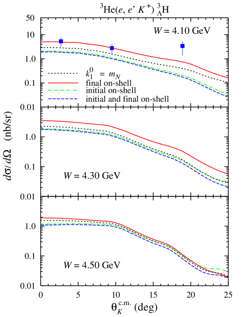
Figure 14: (Color online) Off-shell effect in the hyperon electroproduction. Notations for the curves and data are as in Fig. 10.

Off-shell effects are also found to be important in the case of electroproduction. This fact is clearly exhibited in Fig. 14, where we can see that the “final hyperon on-shell” assumption can nicely shift the cross section upward to reproduce the experimental data at $\theta_{K}^{\rm c.m.}=2.7^{\circ}$ and $9.5^{\circ}$. Obviously, this finding is in contrast to the phenomenon observed in the pion photoproduction off ³He tiator2 , where the assumption that the initial nucleon is on-shell yields a better agreement with experimental data. However, the present finding can be understood as follows: The hyperon binding energy in the hypertriton is much weaker than the binding energy of the nucleon in the ³He. Therefore, shifting the hyperon in the final state closer to its mass-shell moves the model closer to reality. The experimental data point at $\theta_{K}^{\rm c.m.}=18.9^{\circ}$ seems, however, to be very difficult to reproduce. Although the elementary cross section at this kinematics slightly increases, the nuclear suppression from the two nuclear wave functions is sufficiently strong to reduce the cross sections at $\theta_{K}^{\rm c.m.}\geq 10^{\circ}$.

At $W=4.30$ GeV and $W=4.50$ GeV the various off-shell assumptions yield quite different phenomena compared to those in the case of photoproduction (compare the two lower panels of Fig. 14 and Fig. 10). In the case of photoproduction the assumption that the final hyperon is on-shell yields the smallest cross sections, whereas the situation is opposite in the case of electroproduction. Again, this behavior originates from the longitudinal terms. As shown by Fig. 15, for all $W$ shown, the longitudinal cross sections are larger than the transverse ones. In the former, the off-shell effects are more profound and the assumption that the hyperon in the final state is on-shell always yields the largest cross section. Such behavior does not show up in the transverse cross sections. In fact, by comparing the transverse cross sections shown in Fig. 15 and in Fig. 10 we can clearly see that the result presented here is still consistent with that of the photoproduction.

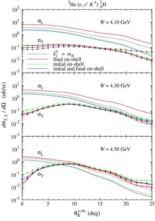
Figure 15: (Color online) Comparison between off-shell effects on the longitudinal and on the transverse cross sections at different values of $W$ and $k^{2}=-0.35$ GeV². Note that for the sake of visibility the transverse cross sections are plotted with lines and points, while the convention for the line types is as in the longitudinal cross sections.

We have also found that although the phenomenon of the dominant longitudinal cross sections originates from the contribution of the missing resonance $D_{13}(1895)$, the fact that the final-hyperon-on-shell assumption always yields the largest cross section is not affected by the omission of this resonance.

IV.3 Future Consideration

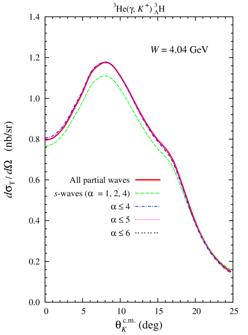
Figure 16: (Color online) Variations of the hypertriton photoproduction cross section at $W=4.04$ GeV as functions of the number of partial waves used and the kaon c.m. angle. Note that the cross sections for $\alpha\leq 5$ and $\alpha\leq 6$ coincide with that of the full calculation (using all partial waves).

The massive numerical integrations in the full calculation using all partial waves described above requires special attention in the future. One way to reduce this task is by limiting the number of the involved elementary amplitudes ${\cal F}_{i}$ given in Appendix A. It has been shown in Ref. Adelseck:1986fb that to a good approximation the “big-big parts” of the Dirac spinors (in our case, the ${\cal F}_{16}$ – ${\cal F}_{20}$) of a special isobar model can be safely neglected. However, the discrepancies between the full calculation and this approximation depends critically on both photon and nucleon energies (see, for instance, Fig. 2 of Ref. Adelseck:1986fb ). Thus, careful inspections in a wide range of kinematics should be previously performed, before we can apply this approximation in the hypertriton production.

Another method which might be of interest is by limiting the number of the partial waves used in the calculation. As shown in Fig. 8, the discrepancy between the results of the full calculation and the $s$-wave approximation can reach about 10%. Therefore, the use of only $s$-wave would not be recommended for a precise calculation. However, the ultimate question is: What is the minimum value of $\alpha$, for which we would obtain the best approximation? To answer this question we have calculated the cross sections at $W=0.4$ GeV by using different numbers of partial waves, from the $s$-wave approximation up to $\alpha=6$, and we demonstrate the result in Fig. 16. From this figure we can immediately conclude that the calculation with $\alpha\leq 4$ would provide a good approximation, whereas by using $\alpha\leq 5$ we could achieve the best result. We note that in the latter the number of non-zero diagonal and interference terms of the components of the wave functions turns out to be 8. Obviously, this method provides a significant CPU-time reduction compared to the full calculation which has 64 non-zero components. In spite of this encouraging result, however, an extensive investigation of this approximation in a wide range of kinematics will need to be addressed in the future, before we can draw a firm conclusion that we really need the triton and hypertriton wave functions with only five partial waves to obtain a precise calculation of the hypertriton production.

V Conclusions and Outlook

We have investigated the photo- and electroproduction of hypertriton on the ³He nucleus by utilizing the modern nuclear wave functions obtained as a solution of the Faddeev equations and the elementary operator KAON-MAID. It has been shown that the proper treatment of the Fermi motion is essential in this process. While the average momentum approximation $\langle{\mbox{\boldmath${k}$}}_{1}\rangle=-\frac{1}{3}{\mbox{\boldmath${Q}$}}$ can partly simulate the Fermi motion, the “frozen nucleon” assumption yields very different results, especially at lower energies. This indicate that the effect of non-localities generated by Fermi motion is important in the electromagnetic production of hypertriton. On the other hand, although the exited meson is a positive kaon, the Coulomb effect induced by its interaction with the hypertriton is found to be negligible. The influence of higher partial waves is also found to be small, in contrast to the finding in the previous work. The off-shell assumption is found to be more important in the case of electroproduction rather than in photoproduction. Our finding indicates that the available experimental data favor the assumption that the initial nucleon is off-shell, whereas the final hyperon is on-shell. This seems to be reasonable, since the hyperon in the hypertriton is less bound than the nucleon in the initial ³He nucleus. The longitudinal cross sections are dominant in the electroproduction process. This originates from the longitudinal terms of the missing resonance $D_{13}(1895)$ in the elementary operator. Nevertheless, the influence of various off-shell assumptions on the longitudinal cross sections is not affected by the exclusion of this resonance. Experimental measurements are strongly required, especially in the case of photoproduction, where we can partly settle the problems of the elementary operator due to the lack of data consistency and of the knowledge on the nucleon resonances as well as hadronic coupling constants. For this case, $W\approx 4.04$ and forward directions represent the recommended kinematics, for which the effects of non-localities, missing resonance $D_{13}(1895)$, as well as various off-shell assumptions are found to be quite significant. Further measurements of the hypertriton electroproduction are obviously useful, especially if we want to explore the role of the longitudinal terms in the elementary operator and to recheck the trend of the angular distribution of the differential cross sections.

Appendix A The Elementary Amplitudes ${\cal F}_{i}$

Here we list the elementary amplitudes ${\cal F}_{1}-{\cal F}_{20}$ defined by Eq. (14). Note that all energies and three-momenta are given in the $\gamma-N$ c.m. or lab system.

$${\cal{F}}_{1} = k_{0}A_{1}+k\cdot q_{K}A_{3}+\{2P\cdot k-k_{0}(m_{N}+m_{Y})\}A_{4}-k^{2}A_{6}~{},$$ (77)

$${\cal{F}}_{2} = -A_{1}-E_{K}A_{3}-(E_{N}+E_{Y}-m_{N}-m_{Y})A_{4}+k_{0}A_{6}~{},$$ (78)

$${\cal{F}}_{3} = A_{3}-A_{6}~{},$$ (79)

$${\cal{F}}_{4} = A_{3}+A_{4}~{},$$ (80)

$${\cal{F}}_{5} = -A_{3}+A_{4}~{},$$ (81)

$${\cal{F}}_{6} = \frac{1}{E_{N}+m_{N}}~{}\Bigl{[}~{}\{2P\cdot k\,(E_{N}-E_{Y})+({\textstyle\frac{1}{2}}k^{2}-k\cdot q_{K})(E_{N}+E_{Y})+P\cdot kk_{0}\}A_{2}$$ (82)

$$\hskip 62.59596pt+(k_{0}E_{K}-k\cdot q_{K})A_{3}+\{k_{0}(E_{N}+E_{Y})-2P\cdot k\}A_{4}$$

$$\hskip 62.59596pt-(k_{0}k\cdot q_{K}-k^{2}E_{K})A_{5}+(k^{2}-k_{0}^{2})A_{6}~{}\Bigr{]}~{},$$

$${\cal{F}}_{7} = \frac{1}{E_{N}+m_{N}}~{}\Bigl{[}\,A_{1}-P\cdot kA_{2}-k_{0}A_{3}-(m_{N}+m_{Y})A_{4}-(k^{2}-k\cdot q_{K})A_{5}+k_{0}A_{6}\,\Bigr{]},$$ (83)

$${\cal{F}}_{8} = \frac{1}{E_{N}+m_{N}}~{}\Bigl{[}-(2P\cdot k+{\textstyle\frac{1}{2}}k^{2}-k\cdot q_{K})A_{2}-k_{0}(A_{3}+A_{4})-k^{2}A_{5}~{}\Bigr{]}~{},$$ (84)

$${\cal{F}}_{9} = \frac{1}{E_{N}+m_{N}}~{}\Bigl{[}~{}(2P\cdot k-{\textstyle\frac{1}{2}}k^{2}+k\cdot q_{K})A_{2}+k_{0}(A_{3}-A_{4})+k^{2}A_{5}~{}\Bigr{]}~{},$$ (85)

$${\cal{F}}_{10} = \frac{1}{E_{Y}+m_{Y}}~{}\Bigl{[}-\{2P\cdot k(E_{N}-E_{Y})+({\textstyle\frac{1}{2}}k^{2}-k\cdot q_{K})(E_{N}+E_{Y})+P\cdot kk_{0}\}A_{2}$$ (86)

$$\hskip 59.75095pt+(k_{0}E_{K}-k\cdot q_{K})A_{3}+\{k_{0}(E_{N}+E_{Y})-2P\cdot k\}A_{4}$$

$$\hskip 59.75095pt+(k_{0}k\cdot q_{K}-k^{2}E_{K})A_{5}+(k^{2}-k_{0}^{2})A_{6}~{}\Bigr{]}~{},$$

$${\cal{F}}_{11} = \frac{1}{E_{Y}+m_{Y}}~{}\Bigl{[}-A_{1}+P\cdot kA_{2}-k_{0}A_{3}+(m_{N}+m_{Y})A_{4}+(k^{2}-k\cdot q_{K})A_{5}+k_{0}A_{6}\,\Bigr{]},$$

$${\cal{F}}_{12} = \frac{1}{E_{Y}+m_{Y}}~{}\Bigl{[}~{}(2P\cdot k+{\textstyle\frac{1}{2}}k^{2}-k\cdot q_{K})A_{2}-k_{0}(A_{3}+A_{4})+k^{2}A_{5}~{}\Bigr{]}~{},$$ (88)

$${\cal{F}}_{13} = \frac{1}{E_{Y}+m_{Y}}~{}\Bigl{[}-(2P\cdot k+k\cdot q_{K}-{\textstyle\frac{1}{2}}k^{2})A_{2}+k_{0}(A_{3}-A_{4})-k^{2}A_{5}~{}\Bigr{]}~{},$$ (89)

$${\cal{F}}_{14} = \frac{1}{E_{N}+m_{N}}~{}\Bigl{[}-A_{1}+(m_{N}+m_{Y})A_{4}~{}\Bigr{]}~{},$$ (90)

$${\cal{F}}_{15} = \frac{1}{E_{Y}+m_{Y}}~{}\Bigl{[}~{}A_{1}-(m_{N}+m_{Y})A_{4}~{}\Bigr{]}~{},$$ (91)

$${\cal{F}}_{16} = \frac{1}{(E_{N}+m_{N})(E_{Y}+m_{Y})}\Bigl{[}-k_{0}A_{1}+k\cdot q_{K}A_{3}+\{2P\cdot k+k_{0}(m_{N}+m_{Y})\}A_{4}-k^{2}A_{6}\Bigr{]},$$

$${\cal{F}}_{17} = \frac{1}{(E_{N}+m_{N})(E_{Y}+m_{Y})}\,\Bigl{[}\,A_{1}-E_{K}A_{3}-(E_{N}+E_{Y}+m_{N}+m_{Y})A_{4}+k_{0}A_{6}\,\Bigr{]}~{},$$

$${\cal{F}}_{18} = \frac{1}{(E_{N}+m_{N})(E_{Y}+m_{Y})}~{}\Bigl{[}~{}A_{3}-A_{6}~{}\Bigr{]}~{},$$ (94)

$${\cal{F}}_{19} = \frac{1}{(E_{N}+m_{N})(E_{Y}+m_{Y})}~{}\Bigl{[}~{}A_{3}+A_{4}~{}\Bigr{]}~{},$$ (95)

$${\cal{F}}_{20} = \frac{1}{(E_{N}+m_{N})(E_{Y}+m_{Y})}~{}\Bigl{[}-A_{3}+A_{4}~{}\Bigr{]}~{}.$$ (96)

Appendix B Normalization of the Three-Body Wave Functions

In the $\gamma+{{}^{3}{\rm He}}\to\pi^{+}+{{}^{3}{\rm H}}$ the initial and final nuclear wave functions are anti-symmetrized. Therefore, in this case it is sufficient to evaluate the elementary production on one of the nucleons and the nuclear amplitude is multiplied with an antisymmetry factor 3 tiator2 . In the hypertriton productions [see Eqs. (2) and (3)], the final nucleus consists of two nucleons and one hyperon. As a consequence, a proper normalization is required, and the anti-symmetry factor has to be recalculated. To this end, we will make use of the method of second quantization, i.e.,

$$\left\{N^{\dagger}(x),N(y)\right\} = \delta_{x,y}~{},$$ (97)

$$\left\{N^{\dagger}(x),\Lambda(y)\right\} = 0~{},$$ (98)

we can show that the normalized ³He and hypertriton wave functions can be written as

$$\left|~{}^{3}{\rm He}~{}\right\rangle = \frac{1}{\sqrt{3!}}~{}\int dxdydz~{}N^{\dagger}(x)N^{\dagger}(y)N^{\dagger}(z)~{}\left|~{}0~{}\right\rangle~{}\Phi_{NNN}(x,y,z)~{},$$ (99)

$$\left|~{}^{3}_{\Lambda}{\rm H}~{}\right\rangle = \frac{1}{\sqrt{2!}}~{}\int dxdydz~{}N^{\dagger}(x)N^{\dagger}(y)\Lambda^{\dagger}(z)~{}\left|~{}0~{}\right\rangle~{}\Phi_{NN\Lambda}(x,y,z)~{},$$ (100)

where $N^{\dagger}(x)$ [$\Lambda^{\dagger}(z)$] represents the nucleon [$\Lambda$] creation operator at the point $x$ [$z$], while $\Phi_{NNN}$ and $\Phi_{NN\Lambda}$ denote the spatial ³He and hypertriton wave functions, respectively.

To create a $\Lambda$ hyperon from a nucleon we need the one-body operator

$${\cal O}(x) = \int dx~{}\Lambda^{\dagger}(x)~{}h(x)~{}N(x)~{},$$ (101)

where $h(x)$ indicates the elementary operator, which can be sandwiched between the ³He and the hypertriton wave functions to give

$$\left\langle~{}^{3}_{\Lambda}{\rm H}~{}\right|~{}{\cal O}(x)~{}\left|~{}^{3}{\rm He}~{}\right\rangle~{}=~{}\frac{1}{\sqrt{12}}\int dxdydz$$

$$\times~{}\Bigl{\{}\Phi^{*}_{NN\Lambda}(y,z,x)~{}h(x)~{}\Phi_{NNN}(x,y,z)-\Phi^{*}_{NN\Lambda}(z,y,x)~{}h(x)~{}\Phi_{NNN}(x,y,z)$$

$$-~{}\Phi^{*}_{NN\Lambda}(x,z,y)~{}h(y)~{}\Phi_{NNN}(x,y,z)+\Phi^{*}_{NN\Lambda}(z,x,y)~{}h(y)~{}\Phi_{NNN}(x,y,z)$$

$$+~{}\Phi^{*}_{NN\Lambda}(x,y,z)~{}h(z)~{}\Phi_{NNN}(x,y,z)-\Phi^{*}_{NN\Lambda}(y,x,z)~{}h(z)~{}\Phi_{NNN}(x,y,z)\Bigr{\}}~{}.$$ (102)

Note that every term in Eq. (102) is integrated over $x$, $y$, and $z$. By making use of the anti-symmetric behavior of $\Phi_{NNN}(x,y,z)$, we can recast Eq. (102) to

$$\left\langle~{}^{3}_{\Lambda}{\rm H}~{}\right|~{}{\cal O}(x)~{}\left|~{}^{3}{\rm He}~{}\right\rangle~{}=~{}\frac{1}{\sqrt{12}}\int dxdydz$$ (103)

$$\times~{}\Bigl{\{}\Phi^{*}_{NN\Lambda}(y,z,x)~{}h(x)~{}\Phi_{NNN}(y,z,x)+\Phi^{*}_{NN\Lambda}(z,y,x)~{}h(x)~{}\Phi_{NNN}(z,y,x)$$

$$+~{}\Phi^{*}_{NN\Lambda}(x,z,y)~{}h(y)~{}\Phi_{NNN}(x,z,y)+\Phi^{*}_{NN\Lambda}(z,x,y)~{}h(y)~{}\Phi_{NNN}(z,x,y)$$

$$+~{}\Phi^{*}_{NN\Lambda}(x,y,z)~{}h(z)~{}\Phi_{NNN}(x,y,z)+\Phi^{*}_{NN\Lambda}(y,x,z)~{}h(z)~{}\Phi_{NNN}(y,x,z)\Bigr{\}}$$

$$= \sqrt{3}\int dxdydz~{}\Phi^{*}_{NN\Lambda}(x,y,z)~{}h(z)~{}\Phi_{NNN}(x,y,z)~{},$$

which shows that the required anti-symmetry factor for the hypertriton production off ³He is $\sqrt{3}$. If we used the above prescription to calculate the amplitude of pion photoproduction on ³He, where the one-body operator in this case may be written as

$${\cal O}(x) = \int dx~{}N^{\dagger}(x)~{}h(x)~{}N(x)~{},$$ (104)

we would obtain

$$\left\langle~{}{{}^{3}{\rm H}}~{}\right|~{}{\cal O}(x)~{}\left|~{}^{3}{\rm He}~{}\right\rangle = 3\int dxdydz~{}\Phi^{*}_{NNN}(x,y,z)~{}h(z)~{}\Phi_{NNN}(x,y,z)~{},$$ (105)

which is consistent with previous work tiator2 .

Appendix C Components of the Elementary Operator Matrix

Here we give the individual components of the matrix [j], defined in Eq. (31) through the relation $J^{\mu}=[\sigma]\,[j]$, which are useful for the numerical calculation of the observables.

$$j_{00} = iN{\cal{F}}_{17}\,\mbox{\boldmath${p}$}_{N}\cdot(\mbox{\boldmath${p}$}_{Y}\times\mbox{\boldmath${k}$})~{},$$ (106)

$$j_{\ell 0} = iN\Bigl{[}{\cal F}_{14}\,\mbox{\boldmath${p}$}_{N}\times\mbox{\boldmath${k}$}+{\cal F}_{15}\,\mbox{\boldmath${p}$}_{Y}\times\mbox{\boldmath${k}$}-{\cal F}_{16}\,\mbox{\boldmath${p}$}_{N}\times\mbox{\boldmath${p}$}_{Y}-\mbox{\boldmath${p}$}_{N}\cdot\mbox{\boldmath${p}$}_{Y}\times\mbox{\boldmath${k}$}\left({\cal F}_{18}\,\mbox{\boldmath${k}$}\,+\right.$$ (107)

$$\left.{\cal F}_{19}\,\mbox{\boldmath${p}$}_{N}+{\cal F}_{20}\,\mbox{\boldmath${p}$}_{Y}\right)\Bigr{]}_{l}~{},$$

$$j_{0m} = N\{({\cal F}_{2}-\mbox{\boldmath${p}$}_{N}\cdot\mbox{\boldmath${p}$}_{Y}\,{\cal F}_{17})\,k_{m}+({\cal F}_{6}+\mbox{\boldmath${p}$}_{Y}\cdot\mbox{\boldmath${k}$}\,{\cal F}_{17})\,p_{N,m}+({\cal F}_{10}+\mbox{\boldmath${p}$}_{N}\cdot\mbox{\boldmath${k}$}\,{\cal F}_{17})\,p_{Y,m}\},~{}~{}~{}~{}$$ (108)

$$j_{\ell m} = A\,\delta_{\ell m}+{B}_{\ell}\,k_{m}+{C}_{\ell}\,p_{N,m}+{D}_{\ell}\,p_{Y,m}~{},$$ (109)

where $\ell,m=x,y,z$, and

$$A = -N\left[{\cal F}_{1}+{\cal F}_{14}\,\mbox{\boldmath${p}$}_{N}\cdot\mbox{\boldmath${k}$}-{\cal F}_{15}\,\mbox{\boldmath${p}$}_{Y}\cdot\mbox{\boldmath${k}$}-{\cal F}_{16}\,\mbox{\boldmath${p}$}_{N}\cdot\mbox{\boldmath${p}$}_{Y}\right]~{},$$ (110)

$${B} = -N\left[({\cal{F}}_{3}-\mbox{\boldmath${p}$}_{N}\cdot\mbox{\boldmath${p}$}_{Y}\;{\cal{F}}_{18})\;\mbox{\boldmath${k}$}+({\cal{F}}_{4}-{\cal{F}}_{14}-\mbox{\boldmath${p}$}_{N}\cdot\mbox{\boldmath${p}$}_{Y}\;{\cal{F}}_{19})\;\mbox{\boldmath${p}$}_{N}\right.$$ (111)

$$\hskip 62.59605pt\left.+~{}({\cal{F}}_{5}+{\cal{F}}_{15}-\mbox{\boldmath${p}$}_{N}\cdot\mbox{\boldmath${p}$}_{Y}\;{\cal{F}}_{20})\;\mbox{\boldmath${p}$}_{Y}\right]~{},$$

$${C} = -N\left[({\cal{F}}_{7}+{\cal F}_{14}+\mbox{\boldmath${p}$}_{Y}\cdot\mbox{\boldmath${k}$}\;{\cal{F}}_{18})\;\mbox{\boldmath${k}$}+({\cal{F}}_{8}+\mbox{\boldmath${p}$}_{Y}\cdot\mbox{\boldmath${k}$}\;{\cal{F}}_{19})\;\mbox{\boldmath${p}$}_{N}\right.$$ (112)

$$\hskip 62.59605pt\left.+~{}({\cal{F}}_{9}+{\cal{F}}_{16}+\mbox{\boldmath${p}$}_{Y}\cdot\mbox{\boldmath${k}$}\;{\cal{F}}_{20})\;\mbox{\boldmath${p}$}_{Y}\right]~{},$$

$${D} = -N\left[({\cal{F}}_{11}+{\cal F}_{15}+\mbox{\boldmath${p}$}_{N}\cdot\mbox{\boldmath${k}$}\;{\cal{F}}_{18})\;\mbox{\boldmath${k}$}+~{}({\cal{F}}_{12}+{\cal F}_{16}+\mbox{\boldmath${p}$}_{N}\cdot\mbox{\boldmath${k}$}\;{\cal{F}}_{19})\;\mbox{\boldmath${p}$}_{N}\right.$$ (113)

$$\hskip 62.59605pt\left.+~{}({\cal{F}}_{13}+\mbox{\boldmath${p}$}_{N}\cdot\mbox{\boldmath${k}$}\;{\cal{F}}_{20})\;\mbox{\boldmath${p}$}_{Y}\right]~{}.$$

Appendix D Useful Kinematical Relations in the Nuclear System

In the $\gamma-^{3}$He laboratory system the energy and momentum of the virtual photon are obtained from

$$k_{0} = \left(W^{2}-M_{\rm He}^{2}-k^{2}\right)/(2M_{\rm He})~{}~{}~{},~{}~{}~{}|\mbox{\boldmath${k}$}|~{}=~{}(k_{0}^{2}-k^{2})^{1/2}~{},$$ (114)

where we denote the total c.m. energy by $W$. On the other hand the energy and momentum of the kaon in the c.m. frame are given by

$$E_{K}^{\rm c.m.} = \left(W^{2}-m_{\Lambda}^{2}+m_{K}^{2}\right)/(2W)~{}~{}~{},~{}~{}~{}|\mbox{\boldmath${q}$}_{K}^{\rm c.m.}|~{}=~{}\{(E_{K}^{\rm c.m.})^{2}-m_{K}^{2}\}^{1/2}~{}.$$ (115)

The corresponding energy and momentum in the laboratory frame are obtained from the following transformation

$$E_{K} = \gamma\Bigl{(}E_{K}^{\rm c.m.}+v|\mbox{\boldmath${q}$}_{K}^{\rm c.m.}|\cos\theta_{\rm c.m.}\Bigr{)}~{}~{}~{},~{}~{}~{}|\mbox{\boldmath${q}$}_{K}|~{}=~{}(E_{K}^{2}-m_{K}^{2})^{1/2}~{},$$ (116)

whereas the kaon scattering angle in the laboratory frame is given by

$$\cos\theta = \gamma\Bigl{(}|\mbox{\boldmath${q}$}_{K}^{\rm c.m.}|\cos\theta_{\rm c.m.}+vE_{K}^{\rm c.m.}\Bigr{)}~{},$$ (117)

where

$$\gamma = (k_{0}+M_{\rm He})/W~{}~{}~{},~{}~{}~{}v~{}=~{}k/(k_{0}+M_{\rm He})~{}.$$ (118)

The formulas below are derived according to Fig. 17 in the laboratory system with Jacobi coordinates. These relations have been used in the numerical calculations.

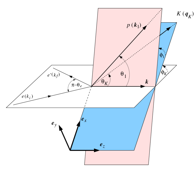
Figure 17: (Color online) Kinematics of the hypertriton electroproduction on ³He. Note that the $x-z$ plane is defined as the $\gamma_{v}-K$ production plane.

We choose the kaon scattering plane as the $xz$-plane, whereas the direction of virtual photon three-momentum defines the $z$-direction, i.e.,

$${k} = k\,\mbox{\boldmath${e}$}_{z}~{}.$$ (119)

Consequently, the initial momentum of the first nucleon and the momentum of the kaon are given by

$$\mbox{\boldmath${k}$}_{1} = k_{1}~{}(\sin\theta_{1}\cos\phi_{1}\mbox{\boldmath${e}$}_{x}+\sin\theta_{1}\sin\phi_{1}\mbox{\boldmath${e}$}_{y}+\cos\theta_{1}\mbox{\boldmath${e}$}_{z})~{},$$ (120)

$$\mbox{\boldmath${q}$}_{K} = q_{K}~{}(\sin\theta_{K}\mbox{\boldmath${e}$}_{x}+\cos\theta_{K}\mbox{\boldmath${e}$}_{z})~{},$$ (121)

while the momentum of the produced hyperon is given by

$$\mbox{\boldmath${k}$}_{1}^{\prime} = \mbox{\boldmath${k}$}_{1}+{\textstyle\frac{2}{3}}\left(\mbox{\boldmath${k}$}-\mbox{\boldmath${q_{K}}$}\right)$$ (122)

$$= (k_{1}\sin\theta_{1}\cos\phi_{1}-{\textstyle\frac{2}{3}}q_{K}\sin\theta_{K})\,\mbox{\boldmath${e}$}_{x}+(k_{1}\sin\theta_{1}\sin\phi_{1})\,\mbox{\boldmath${e}$}_{y}$$

$$+(k_{1}\cos\theta_{1}+{\textstyle\frac{2}{3}}k-{\textstyle\frac{2}{3}}q_{K}\cos\theta_{K})\,\mbox{\boldmath${e}$}_{z}$$

$$\equiv k_{1}^{\prime}\left(\sin\theta_{1}^{\prime}\cos\phi_{1}^{\prime}\,\mbox{\boldmath${e}$}_{x}+\sin\theta_{1}^{\prime}\sin\phi_{1}^{\prime}\,\mbox{\boldmath${e}$}_{y}+\cos\theta_{1}^{\prime}\,\mbox{\boldmath${e}$}_{z}\right)~{}.$$

From this we can derive the following expressions for vector and scalar products of the photon (${k}$), nucleon ($\mbox{\boldmath${k}$}_{1}$), kaon ($\mbox{\boldmath${q}$}_{K}$), and hyperon ($\mbox{\boldmath${k}$}_{1}^{\prime}$) momenta,

$$\mbox{\boldmath${q}$}_{K}\cdot\mbox{\boldmath${k}$} = q_{K}k~{}\cos\theta_{K}~{},$$ (123)

$$\mbox{\boldmath${k}$}_{1}\cdot\mbox{\boldmath${k}$} = k_{1}k~{}\cos\theta_{1}~{},$$ (124)

$$\mbox{\boldmath${q}$}_{K}\cdot\mbox{\boldmath${k}$}_{1} = q_{K}k_{1}~{}(\sin\theta_{K}~{}\sin\theta_{1}~{}\cos\phi_{1}+\cos\theta_{K}~{}\cos\theta_{1})~{},$$ (125)

$$\mbox{\boldmath${k}$}_{1}\cdot(\mbox{\boldmath${k}$}-\mbox{\boldmath${q}$}_{K}) = k_{1}k~{}\cos\theta_{1}-k_{1}q_{K}~{}(\sin\theta_{K}~{}\sin\theta_{1}~{}\cos\phi_{1}+\cos\theta_{K}~{}\cos\theta_{1})~{},$$ (126)

$$\mbox{\boldmath${q}$}_{K}\times\mbox{\boldmath${k}$}_{1} = q_{K}k_{1}~{}[-\sin\theta_{1}\sin\phi_{1}~{}\cos\theta_{K}~{}\mbox{\boldmath${e}$}_{x}+(\sin\theta_{1}\cos\phi_{1}~{}\cos\theta_{K}$$ (127)

$$-\sin\theta_{K}~{}\cos\theta_{1})~{}\mbox{\boldmath${e}$}_{y}+\sin\theta_{1}~{}\sin\phi_{1}~{}\sin\theta_{K}~{}\mbox{\boldmath${e}$}_{z}]~{},$$

$$\mbox{\boldmath${k}$}\times\mbox{\boldmath${q}$}_{K} = kq_{K}~{}\sin\theta_{K}~{}\mbox{\boldmath${e}$}_{y}~{},$$ (128)

$$\mbox{\boldmath${k}$}_{1}\times\mbox{\boldmath${k}$} = k_{1}k~{}\sin\theta_{1}~{}(\sin\phi_{1}\mbox{\boldmath${e}$}_{x}-\cos\phi_{1}\mbox{\boldmath${e}$}_{y})~{},$$ (129)

$$\mbox{\boldmath${k}$}_{1}^{\prime}\times\mbox{\boldmath${k}$}_{1} = {\textstyle\frac{2}{3}}~{}(\mbox{\boldmath${k}$}\times\mbox{\boldmath${k}$}_{1}-\mbox{\boldmath${q}$}_{K}\times\mbox{\boldmath${k}$}_{1})~{},$$ (130)

$$k_{1}^{\prime} = \left\{{k}_{1}^{2}+{\textstyle\frac{4}{3}}(\mbox{\boldmath${k}$}_{1}\cdot\mbox{\boldmath${k}$}-\mbox{\boldmath${k}$}_{1}\cdot\mbox{\boldmath${q}$}_{K})+{\textstyle\frac{4}{9}}({k}^{2}+{q}_{K}^{2}-2\mbox{\boldmath${k}$}\cdot\mbox{\boldmath${q}$}_{K})\right\}^{1/2}~{},$$ (131)

$$\theta_{1}^{\prime} = \cos^{-1}\Bigl{[}\left\{k_{1}\cos\theta_{1}+{\textstyle\frac{2}{3}}(k-q_{K}\cos\theta_{K})\right\}/k_{1}^{\prime}\Bigr{]}~{},$$ (132)

$$\phi_{1}^{\prime} = \sin^{-1}\{(k_{1}\sin\theta_{1}\sin\phi_{1})/(k_{1}^{\prime}\sin\theta_{1}^{\prime})\}~{}.$$ (133)

References

- (1) K. Miyagawa, private communication.
- (2) I. R. Afnan and B. F. Gibson, Phys. Rev. C. 47, 1000 (1993).
- (3) C. B. Dover, H. Feshbach, and A. Gal, Phys. Rev. C 51, 541 (1995).
- (4) M. Juric et al., Nucl. Phys. B 52, 1 (1973).
- (5) G. Keyes et al., Phys. Rev. Lett. 20, 819 (1968); ibid., Phys. Rev. D 1, 66 (1970); G. Keyes, J. Sacton, J. H. Wickens, and M. M. Block, Nucl. Phys. B67, 269 (1973); R. E. Phillips and J. Schneps, Phys. Rev. Lett. 20, 1383 (1968); ibid., Phys. Rev. 180, 1307 (1969); G. Bohm et al., Nucl. Phys. B16, 46 (1970).
- (6) K. Miyagawa and W. Glöckle, Phys. Rev. C 48, 2576 (1993).
- (7) K. Miyagawa, H. Kamada, W. Glöckle, and V. Stoks, Phys. Rev. C 51, 2905 (1995).
- (8) J. Golak et al., Phys. Rev. C 55, 2196 (1997); A. Cobis, A. S. Jensen and D. V. Fedorov, J. Phys. G 23, 401 (1997); H. Kamada, J. Golak, K. Miyagawa, H. Witala and W. Gloeckle, Phys. Rev. C 57, 1595 (1998); J. Golak, H. Witala, K. Miyagawa, H. Kamada and W. Gloeckle, Phys. Rev. Lett. 83, 3142 (1999); K. Tominaga and T. Ueda, Nucl. Phys. A 693, 731 (2001); H. W. Hammer, Nucl. Phys. A 705, 173 (2002); H. Nemura, Y. Akaishi and Y. Suzuki, Phys. Rev. Lett. 89, 142504 (2002); D. V. Fedorov and A. S. Jensen, Nucl. Phys. A 697, 783 (2002); Y. Fujiwara, K. Miyagawa, M. Kohno and Y. Suzuki, Phys. Rev. C 70, 024001 (2004).
- (9) A. G. Reuber, K. Holinde, and J. Speth, Czech. J. Phys. 42, 1115 (1992); K. Holinde, Nucl. Phys. A 547, 255c (1992).
- (10) P. M. M. Maessen, Th. A. Rijken, and J. J. de Swart, Phys. Rev. C 40 (1989) 2226.
- (11) V. I. Komarov, A. V. Lado, and Yu. N. Uzikov, J. Phys. G 21, L69 (1995).
- (12) A. Gardestig, Z. Phys. A 357, 101 (1997).
- (13) T. Mart, L. Tiator, D. Drechsel, and C. Bennhold, Nucl. Phys. A640, 235 (1998).
- (14) T. Mart, Ph.D. Thesis, Universität Mainz, 1996 (unpublished).
- (15) R. A. Brandenburg, Y. E. Kim, and A. Tubis, Phys. Rev. C 12, 1368 (1975).
- (16) J. G. Congleton, J. Phys. G 18, 339 (1992).
- (17) R. A. Williams, C.-R. Ji, and S. R. Cotanch, Phys. Rev. D 41, 1449 (1990); Phys. Rev. C 43, 452 (1991); Phys. Rev. C 46, 1617 (1992).
- (18) F. Dohrmann et al., Phys. Rev. Lett. 93, 242501 (2004).
- (19) See the upper panel of Fig. 3 of Ref. Dohrmann:2004xy .
- (20) See the lower panel of Fig. 3 of Ref. Dohrmann:2004xy .
- (21) V. G. J. Stoks, R. A. M. Klomp, C. P. F. Terheggen, and J. J. de Swart, Phys. Rev. C 49, 2950 (1994).
- (22) T. Mart and C. Bennhold, Phys. Rev. C 61, 012201(R) (1999); T. Mart, Phys. Rev. C 62, 038201 (2000); C. Bennhold, H. Haberzettl and T. Mart, arXiv:nucl-th/9909022; T. Mart, C. Bennhold, H. Haberzettl, and L. Tiator, http://www.kph.uni-mainz.de/MAID/kaon/kaonmaid.html.
- (23) H. Yamamura, K. Miyagawa, T. Mart, C. Bennhold, W. Glöckle, and H. Haberzettl, Phys. Rev. C 61, 014001 (1999); K. Miyagawa, T. Mart, C. Bennhold and W. Glöckle, Phys. Rev. C 74, 034002 (2006); A. Salam, K. Miyagawa, T. Mart, C. Bennhold and W. Glöckle, Phys. Rev. C 74, 044004 (2006).
- (24) H. Haberzettl, C. Bennhold, T. Mart, and T. Feuster, Phys. Rev. C 58, R40 (1998).
- (25) M. Q. Tran et al., Phys. Lett. B 445, 20 (1998).
- (26) G. Niculescu et al., Phys. Rev. Lett. 81, 1805 (1998).
- (27) R. M. Mohring et al., Phys. Rev. C 67, 055205 (2003).
- (28) P. Brauel et al., Z. Phys. C 3, 101 (1979).
- (29) A. Bleckman et al., Z. Phys. 239, 1 (1970).
- (30) K. H. Glander et al., Eur. Phys. J. A 19, 251 (2004).
- (31) M. Q. Tran et al., Phys. Lett. B 445, 20 (1998).
- (32) R. Bradford et al., Phys. Rev. C 73, 035202 (2006).
- (33) References for older data are given, e.g., in Ref. saphir .
- (34) T. Mart and A. Sulaksono, Phys. Rev. C 74, 055203 (2006).
- (35) See the Introduction part of P. Bydzovsky and T. Mart, Phys. Rev. C 76, 065202 (2007); and P. Bydzovsky, M. Sotona, T. Motoba, K. Itonaga, K. Ogawa and O. Hashimoto, arXiv:0706.3836 [nucl-th].
- (36) A. de Shalit and I. Thalmi, Nuclear Shell Theory (Academic Press, New York, 1963).
- (37) L. Tiator and D. Drechsel, Nucl. Phys. A 360, 208 (1981).
- (38) G. F. Chew, M. L. Goldberger, F. E. Low, and Y. Nambu, Phys. Rev. 106, 1345 (1957).
- (39) L. Tiator, A. K. Rej, and D. Drechsel, Nucl. Phys. A 333, 343 (1980); L. Tiator, Nucl. Phys. A 364, 189 (1981).
- (40) L. Tiator, Ph. D. Thesis, Universität Mainz, 1980 (unpublished).
- (41) R. A. Adelseck, C. Bennhold and L. E. Wright, Phys. Rev. C 32, 1681 (1985).