Multi-BPS D-vortices

Abstract

We investigate the BPS configuration of the multi D-vortices produced from the D2${\bar{\rm D}}$2 system. Based on the DBI-type action with a Gaussian-type runaway potential for a complex tachyon field, the BPS limit is achieved when the tachyon profile is thin. The solution states randomly-distributed $n$ static D-vortices with zero interaction. With the obtained BPS configuration, we derive the relativistic Lagrangian which describes the dynamics of free massive D-vortices. We also discuss the 90^∘ and 180^∘ scattering of two identical D-vortices, and present its implications on the reconnection in the dynamics of cosmic superstrings.

I Introduction

The Bogomolnyi-Prasad-Sommerfield (BPS) limit of solitons Bogomolny:1975de has been attractive in its nature and tractability of dynamics. The BPS limit is characterized by a minimum-energy configuration of a static soliton which is a solution to the first-order Bogomolnyi equation. The dynamics of multi-BPS solitons is characterized by no interaction. The BPS solitons do not exert any forces to nearby solitons, so they move freely until they collide.

Recently D- and DF-strings have attracted attention as new candidates of cosmic superstrings which produce Y-junctions Copeland:2003bj ; Dvali:2003zj . Concerning string cosmology, such superstrings generated through the decay of D3${\bar{\rm D}}$3 system are intriguing since the separated D${\bar{\rm D}}$ provides a natural setting for an inflationary epoch Dvali:1998pa and can be employed in a string cosmological model with fluxes and moduli stabilization Kachru:2003sx . Once D-strings are produced, understanding their dynamics Jackson:2004zg ; Copeland:2006eh is important in order to see the distinctive evolution between cosmic strings and cosmic superstrings.

In this work, we consider D-vortices which are produced in the coincidence limit of D2${\bar{\rm D}}$2. (The model is equivalent to parallel D-strings produced from D3${\bar{\rm D}}$3.) We consider an effective field theory of a complex tachyon field described by a Dirac-Born-Infeld (DBI) type action, which reflects the instability of D${\bar{\rm D}}$ system Sen:2003tm ; Garousi:2004rd . In the context of effective field theory, D0-branes from D2${\bar{\rm D}}$2 have been obtained as D-vortex configurations in (1+2)-dimensions Jones:2002si ; Kim:2005tw ; Cho:2005wp .

In this article, we present a precise process obtaining the BPS configuration for multi D-vortices and their moduli-space dynamics based on Refs. Kim:2006xi ; Cho:2007jf . The BPS limit is possibly obtained with a Gaussian-type potential for the tachyon, and the BPS configuration expresses infinitely thin D-vortices randomly-distributed on a plane Kim:2006xi . We show also that such a configuration reproduces the BPS sum rule and descent relation correctly. With the obtained BPS solution, we derive a relativistic Lagrangian which describes correctly the dynamics of the multi BPS D-vortices Cho:2007jf . The BPS D-vortices behave as free point-like particles with mass identified with the D0-brane tension when they are separated. We show that the scattering of two identical BPS D-vortices exhibits the 90^∘ scattering and the 180^∘ (equivalently 0^∘) scattering, which corresponds individually to the reconnection and the passing through of D-strings when it is applied to the dynamics of cosmic superstrings.

The article is organized as following. In Section II, we review the Nielsen-Olesen vortex in the Abelian-Higgs model and present a derivation of its BPS bound. In Section III, we present precise BPS conditions and obtain the BPS configuration of multi D-vortices. In Section IV, we derive the classical moduli-space dynamics of these BPS D-vortices. We conclude in Section V.

II Ablian-Higgs model and BPS limit

In this section, we briefly review the Nielsen-Olesen vortex in Abelian-Higgs system, and its BPS properties. The Abelian-Higgs model is described by a complex scalar field $\phi$ and a U(1) gauge field $A^{\mu}$. In flat $(1+2)$ dimensions, the action reads

$$S=\int dtd^{2}x\left[-\frac{1}{2}\overline{D_{\mu}\phi}D^{\mu}\phi-V(\phi)-\frac{1}{4}F_{\mu\nu}F^{\mu\nu}\right],$$ (1)

where $F_{\mu\nu}=\partial_{\mu}A_{\nu}-\partial_{\nu}A_{\mu}$ is the field-strength tensor of the gauge field and $D_{\mu}=\partial_{\mu}-iA_{\mu}$ is the covariant derivative. The electric component of the field strength is given by $E_{i}=F_{ti}=\partial_{t}A_{i}-\partial_{i}A_{t}$ and the magnetic component is by $B=\partial_{x}A_{y}-\partial_{y}A_{x}$.

The Nielsen-Olesen vortex is produced during the phase transition accompanied by spontaneous symmetry-breaking with a temperature-dependent effective potential,

$$V_{\rm eff}(\phi,T)=\frac{\alpha\lambda}{4}T^{2}|\phi|^{2}+V(\phi),\quad V(\phi)=\frac{\lambda}{8}(|\phi|^{2}-\eta^{2})^{2},$$ (2)

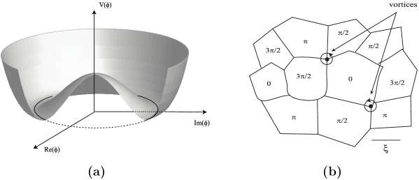
where $\eta$ is the symmetry-breaking scale, and $\lambda$ is the self-coupling constant, and $\alpha$ is a dimensionless constant. The effective potential has a temperature-dependent effective mass $m_{\rm eff}^{2}(T)=\lambda(\alpha T^{2}-\eta^{2})/2$. At sufficiently high temperatures, $T>T_{c}\equiv\eta/\sqrt{\alpha}$, $m_{\rm eff}^{2}$ is positive, and the effective potential $V_{\rm eff}$ has the minimum at $|\phi|=0$ which is the vacuum state. This vacuum is invariant under the rotation in the field space, and the U(1) symmetry is preserved. As the temperature drops, $m_{\rm eff}^{2}$ becomes negative, $V_{\rm eff}$ develops minima at $|\phi|=|m_{\rm eff}|/\sqrt{\lambda}$, and the phase transition undergoes. When the phase transition is completed at zero temperature, the system is described by the unperturbed potential $V$. The vacuum manifold is an ${\rm S}^{1}$ of radius $|\phi|=\eta$ in the phase field space as shown in Fig. 1-(a). Since the vacuum is superselected by a point in this ${\rm S}^{1}$ and is not invariant under the rotation, the continuous U(1) symmetry is broken.

As a result of phase transition, a vortex configuration can be formed. The field configuration of the vortex has vanishing field $\phi$ (i.e., the symmetric state) at the center, and the phase of $\phi$ increases by $2\pi n$ along a circle enclosing the center counter-clockwise. Here, $n$ is a nonzero integer which is interpreted as a winding number. The negative value of $n$ represents an anti-vortex.

Such a nontrivial vortex configuration is guaranteed by the Kibble mechanism Kibble:1976sj . As the phase transition proceeds, the value of $\phi$ in the spatial points transits from the symmetric phase (zero) to the broken symmetric one (nonzero). The domains in the physical space are correlated only by a causal length $\xi$ which is not larger than the horizon scale at that moment. Therefore, each domain takes a different phase value in the vacuum manifold. When the phases of domains are aligned in such a way to wrap the circle of the vacuum manifold, it is irresistible to have a boundary point of the domains, where the field vanishes to avoid a singularity. Thereby, a vortex configuration is achieved. (See Fig. 1-(b).) Such a nontrivial configuration is called the “vortex configuration” which exhibits $\phi=0$ at the center and $\phi=\eta$ in the asymptotic region. When the gauge field is involved, it is called the Nielsen-Olesen vortex Nielsen:1973cs . Once vortices are formed in space, it is topologically stable since erasing the vortex configuration requires the rearrangement of the field structure in entire infinite space.

Figure 1: (a) Plot of the unperturbed potential. (b) Plot of mapping for a complex scalar field and vortex formation.

Now, let us discuss the BPS picture of the Nielsen-Olesen vortex MS . We assume a static-field configuration and the Weyl gauge, $A_{0}=0$. Then, the Bogomolnyi bound for the vortex is saturated when $\lambda=1$. The energy-momentum tensor from the action (1) is

$$T_{\mu\nu}=\frac{1}{2}\left(\overline{D_{\mu}\phi}D_{\nu}\phi+\overline{D_{\nu}\phi}D_{\mu}\phi\right)+g^{\alpha\beta}F_{\mu\alpha}F_{\nu\beta}+g_{\mu\nu}{\cal L}.$$ (3)

After rescaling $\eta x^{\mu}\to x^{\mu}$, $\phi/\eta\to\phi$, and $A^{\mu}/\eta\to A^{\mu}$, the Ginzburg-Landau energy evaluated from the action (1) becomes

$$E = \int d^{2}x(-T^{0}_{0})$$ (4)

$$= \frac{1}{2}\int d^{2}x\left[B^{2}+\overline{D_{i}\phi}D_{i}\phi+\frac{1}{4}(\bar{\phi}\phi-1)^{2}\right]$$ (5)

$$= \frac{1}{2}\int d^{2}x\left\{\left[B\pm\frac{1}{2}\left(\bar{\phi}\phi-1\right)\right]^{2}+|(D_{x}\pm iD_{y})\phi|^{2}\pm B\mp\epsilon_{ij}\partial_{i}J_{j}\right\}$$ (6)

$$\geq \frac{1}{2}|\Phi|,$$ (7)

where $J_{i}=i\left({\bar{\phi}}D_{i}\phi-\phi{\overline{D_{i}\phi}}\right)/2$ in Eq. (6) is the conserved U(1) current, the upper/lower sign is for vortex/anti-vortex in Eq. (6), and $\Phi$ in Eq. (7) is magnetic flux,

$$\Phi\equiv\int d^{2}xB.$$ (8)

The U(1) current vanishes at spatial infinity and does not contribute to the energy after integration. For an object carrying magnetic flux, the equality holds and the minimum-energy configuration is achieved when the first two squared terms vanish, which provides two Bogomolnyi equations,

$$(D_{x}\pm iD_{y})\phi=0,\quad B\pm\frac{1}{2}\left(\bar{\phi}\phi-1\right)=0.$$ (9)

Since the magnetic flux is quantized and uncharged by small fluctuation, these two first-order equations should reproduce second-order (Euler-Lagrange) field equations associated with the original action (1),

$$D^{i}D_{i}\phi-\frac{1}{2}(\bar{\phi}\phi-1)\phi=0,\quad\epsilon_{ij}\partial^{j}B+\frac{i}{2}(\bar{\phi}D_{i}\phi-\phi\overline{D_{i}\phi})=0.$$ (10)

Therefore, when the Nielsen-Olesen vortex (or anti-vortex) carrying magnetic flux $\Phi=2n$ satisfies the Bogomolnyi equations (10), the Ginzburg-Landau energy in Eq. (6) saturates the Bogomolnyi bound in Eq. (7) and shows a so-called BPS sum rule,

$$E=E_{n}=\pi|n|.$$ (11)

Note that, in the Bogomolnyi limit of $\lambda=1$, the mass of gauge field ($\eta$) and that of Higgs field ($\sqrt{\lambda}\eta$) become the same, and this property is consistent with the observation that the action (1) is bosonic sector of the $N=2$ supersymmetric extension of the Abelian-Higgs model Di Vecchia:1977bs .

Let us discuss the $n$ static vortex configurations superimposed at the origin for arbitrary $\lambda$ in what follows. From Eq. (3), its stress components are rewritten as

$$T^{x}_{\;x} = \frac{1}{4}\left[(\overline{D_{x}+iD_{y})\phi}(D_{x}-iD_{y})\phi+(\overline{D_{x}-iD_{y})\phi}(D_{x}+iD_{y})\phi\right]$$ (12)

$$+\frac{1}{2}\left[B+\frac{\sqrt{\lambda}}{2}\left({\bar{\phi}}\phi-\eta^{2}\right)\right]\left[B-\frac{\sqrt{\lambda}}{2}\left({\bar{\phi}}\phi-\eta^{2}\right)\right],$$

$$T^{y}_{\;y} = -\frac{1}{4}\left[(\overline{D_{x}+iD_{y})\phi}(D_{x}-iD_{y})\phi+(\overline{D_{x}-iD_{y})\phi}(D_{x}+iD_{y})\phi\right]$$ (13)

$$+\frac{1}{2}\left[B+\frac{\sqrt{\lambda}}{2}\left({\bar{\phi}}\phi-\eta^{2}\right)\right]\left[B-\frac{\sqrt{\lambda}}{2}\left({\bar{\phi}}\phi-\eta^{2}\right)\right],$$

$$T^{x}_{\;y} = \frac{i}{4}\left[(\overline{D_{x}\pm iD_{y})\phi}(D_{x}\mp iD_{y})\phi-(\overline{D_{x}\mp iD_{y})\phi}(D_{x}\pm iD_{y})\phi\right].$$ (14)

It is manifest that the solutions to the Bogomolnyi equations (9) make these stress components vanish in the BPS limit ($\lambda=1$). It means that the attractions and the repulsions are completely canceled out everywhere for the static BPS Nielsen-Olesen vortex configuration of arbitrary shape and winding number $n$.

For the $n$ superimposed vortices, the scalar and the gauge field which satisfy the Euler-Lagrange equations (10), have asymptotic expressions in cylindrical coordinates $(\rho,\theta)$ as

$$\phi(\rho)\sim 1-\frac{A_{\rm s}}{2\pi}K_{0}(\sqrt{\lambda}\rho),\quad A_{\theta}(\rho)\sim n-\frac{A_{\rm m}}{2\pi}\rho K_{1}(\rho),$$ (15)

where $K_{n}$ is the modified Bessel function. The coefficients $A_{\rm s}$ and $A_{\rm m}$ associated with the decay of scalar and magnetic fields, are only determined numerically for nonBPS vortices de Vega:1976mi ; Speight:1996px , but, for BPS vortices, are predicted analytically by the argument based on string duality Tong:2002rq .

As it was mentioned previously for the general BPS configuration, a defining property of the BPS configuration is implied in the interaction of vortices. Consider two unit-winding vortices with a separation $s\gg 1$. The interaction energy $E_{\rm int}(s)$ is the total energy $E$ minus $2E_{1}$. There are two contributions to $E_{\rm int}$ coming from the scalar field and the magnetic field. At large separations, the interaction energy is evaluated from Eq. (15) and obtained Bettencourt:1994kf by

$$E_{\rm int}(s)=-\frac{A_{\rm s}^{2}}{2\pi}K_{0}(\sqrt{\lambda}s)+\frac{A_{\rm m}^{2}}{2\pi}K_{0}(s).$$ (16)

Naturally, the scalar field induces attraction while the magnetic field does repulsion. For $\lambda=1$, $A_{\rm s}=A_{\rm m}$ Speight:1996px ; Tong:2002rq , which means the interaction energy vanishes. It confirms that there is no interaction between static vortices, when the BPS limit is saturated. Since the interaction scale is of order $1/v$ and there does not exist gapless radiation in the Abelian-Higgs model, the vortices move freely until the separation becomes small enough ($1/v>1$). For $\lambda<1$, the scalar term dominates and the vortices attract. For $\lambda>1$, the magnetic term dominates and the vortices repel.

As shown in the discussion based on the stress components (12)–(14) of the energy-momentum tensor, the interaction story in the BPS limit can be extended to the $n$-vortex configurations and be figured out also from the energy relation (the BPS sum rule) (11). Consider an $n$-winding vortex. From the energy relation, the interaction energy is given by $E_{\rm int}=E_{n}-nE_{1}=0$. This means that well-separated $n$ unit-winding vortices do not interact to accumulate to a single $n$-winding vortex. In addition, a single $n$-winding vortex does not dissociate to $n$ unit-winding vortices, either. Therefore, there will be no interaction among vortices. For $\lambda<1$, $E_{n}<nE_{1}$, and the vortices attract to accumulate. For $\lambda<1$, $E_{n}>nE_{1}$, and the vortices repel to move apart.

The story so far is about the properties of BPS Nilesen-Olesen vortices. The concept of the BPS limit in what follows would more precisely specified by following three conditions.

(C1) The static configurations are obtained from first-order Bogomolnyi equations: These equations are usually obtained by vanishing stress components of the energy-momentum tensor, $T^{i}_{j}=0$, or by minimizing the energy.

(C2) These BPS configurations should satisfy Euler-Lagrange equations: For the case of static Nielsen-Olesen vortex, it is automatic because the Bogomolnyi equations reproduce Euler-Lagrange equations with $\lambda=1$.

(C3) The BPS configurations provide the BPS-sum rule as seen from Eq. (11): This states that the integrated energy is given by a product of a certain topological charge, for example, the winding number $n$ of vortex.

III D${\bar{\bf D}}$ System and BPS Limit of Multi-D-vortices

The properties of D$(p-2)$ (or ${\bar{\rm D}}(p-2)$) produced from the system of D$p{\bar{\rm D}}p$ in the coincidence limit is described by an effective field theory of a complex tachyon field, $T=\tau\exp(i\chi)$, and two Abelian gauge fields of U(1)$\times$U(1) gauge symmetry, $A^{\mu}$ and $C^{\mu}$. A candidate is a DBI type action Sen:2003tm ; Garousi:2004rd

$$S=-{\cal T}_{p}\int d^{p+1}x\,V(\tau)\left[\,\sqrt{-\det(X^{+}_{\mu\nu})}+\sqrt{-\det(X^{-}_{\mu\nu})}\,\,\right],$$ (17)

where ${\cal T}_{p}$ is the tension of the D$p$-brane, $V(\tau)$ is a runaway-type potential which is normalized as $V(\tau=0)=1$ and vanishes as $V(\tau\to\infty)\to 0$, and

$$X^{\pm}_{\mu\nu}=g_{\mu\nu}+F_{\mu\nu}\pm C_{\mu\nu}+({\overline{D_{\mu}T}}D_{\nu}T+{\overline{D_{\nu}T}}D_{\mu}T)/2$$ (18)

with $F_{\mu\nu}=\partial_{\mu}A_{\nu}-\partial_{\nu}A_{\mu},~{}C_{\mu\nu}=\partial_{\mu}C_{\nu}-\partial_{\nu}C_{\mu},~{}\mbox{and}~{}D_{\mu}T=(\partial_{\mu}-2iC_{\mu})T.$

In this work, we shall consider only D${\bar{\rm D}}$ of $p=3$ in type IIB string theory where both gauge fields $A^{\mu}$ and $C^{\mu}$ are turned off. Then, we obtain codimension-two object, D-strings (D1-branes). Since we are interested in straight multi-D-strings stretched parallel to an axis, parallel one-dimensional D-strings in three dimensions from D3${\bar{\rm D}}$3 can equivalently be treated as point-like D-vortices in two dimensions. Considering a static-tachyon configuration for multi-D-vortices in the $(x,y)$-plane without quantized magnetic flux, we have $F_{\mu\nu}=0$, $C_{\mu\nu}=0$, and

$$T=T(x^{i}),\quad(i=1,2),$$ (19)

and shall precisely derive the BPS limit of static multi-D-vortices following the three BPS requirements presented in the previous section.

(C1) Bogomolnyi equation and its BPS solutions: Plugging the tachyon (19) in the stress components of the energy-momentum tensor leads to

$$T^{i}_{\;j}=-\frac{2{\cal T}_{2}V}{\sqrt{1+S_{mm}-\frac{1}{2}A_{mn}^{2}}}\left[\delta_{ij}-\left(S_{ij}-\delta_{ij}S_{kk}\right)+\left(A_{ik}A_{jk}-\frac{\delta_{ij}}{2}A_{kl}^{2}\right)\right],$$ (20)

where

$$S_{ij}\left(A_{ij}\right)=\frac{1}{2}\left(\partial_{i}{\overline{T}}\partial_{j}T\pm\partial_{j}{\overline{T}}\partial_{i}T\right).$$ (21)

Considering the pressure difference and reshuffling the terms, we obtain

$$T^{x}_{\;x}-T^{y}_{\;y}=\frac{{\cal T}_{2}V}{\sqrt{1+S_{ii}-\frac{1}{2}A_{ij}^{2}}}\left[(\overline{\partial_{x}T+i\partial_{y}T})(\partial_{x}T-i\partial_{y}T)+(\overline{\partial_{x}T-i\partial_{y}T})(\partial_{x}T+i\partial_{y}T)\right].$$ (22)

It vanishes when the first-order Cauchy-Riemann equation,

$$(\partial_{x}\pm i\partial_{y})T=0,\qquad(\,\partial_{x}\ln\tau=\pm\partial_{y}\chi\;{\rm and}\;\partial_{y}\ln\tau=\mp\partial_{x}\chi\,),$$ (23)

is satisfied, and thus we may employ this as the Bogomolnyi equation. Applying the Bogomolnyi equation to the off-diagonal stress component $T^{x}_{\;y}$, we confirm that it vanishes

$$T^{x}_{\;y} = i\frac{{\cal T}_{2}V}{2\sqrt{1+S_{ii}-\frac{1}{2}A_{ij}^{2}}}\left[(\overline{\partial_{x}T\pm i\partial_{y}T})(\partial_{x}T\mp i\partial_{y}T)-(\overline{\partial_{x}T\mp i\partial_{y}T})(\partial_{x}T\pm i\partial_{y}T)\right]\stackrel{{\scriptstyle(\ref{BPS})}}{{=}}0.$$ (24)

We solve the Bogomolnyi equation (23) and obtain static BPS configuration of $n$ static D-vortices located randomly in the $(x,y)$-plane. The ansatz of the tachyon field is

$$\displaystyle{T=\tau(x,y)e^{i\sum_{p=1}^{n}\theta_{p}},}\qquad\theta_{p}=\tan^{-1}\frac{y-y_{p}}{x-x_{p}},$$ (25)

where ${\bf x}_{p}=(x_{p},y_{p})$ $(p=1,2,...,n)$ denotes the position of $p$-th D-vortex. Inserting the ansatz (25) into the Bogomolnyi equation (23), we obtain the solution for the tachyon amplitude,

$$\tau(x,y)=\prod_{p=1}^{n}\tau_{{\rm BPS}}|{\bf x}-{\bf x}_{p}|,$$ (26)

where $\tau_{{\rm BPS}}$ is a constant. Plugging the ansatz (25) and solution (26) into the pressure components, we obtain

$$-T^{x}_{\;x}=-T^{y}_{\;y}=2{\cal T}_{2}V.$$ (27)

In the zero-radius limit of D-vortices, $\tau_{{\rm BPS}}\rightarrow\infty$, the potential $V$ vanishes everywhere except the centers of vortices since $V$ is a runaway type. Therefore, the pressure components vanish in this limit everywhere except the vortex positions with $-T^{x}_{\;x}|_{{\bf x}={\bf x}_{p}}=-T^{y}_{\;y}|_{{\bf x}={\bf x}_{p}}=2{\cal T}_{2}$. As a result, a candidate solution to the Bogomolnyi equation (23) is obtained by taking the thin limit,

$$\tau(x,y)=\lim_{\tau_{{\rm BPS}}\to\infty}\prod_{p=1}^{n}\tau_{{\rm BPS}}|{\bf x}-{\bf x}_{p}|=\left\{\begin{array}[]{ll}0,&\hbox{at each ${{\bf x}}_{p}$}\,,\\ \infty,&\hbox{elsewhere}.\\ \end{array}\right.$$ (30)

(C2) Euler-Lagrange equation: For the nontrivial-tachyon configuration, the Euler-Lagrange equation is equivalent to the conservation of the energy-momentum tensor. Since $T^{x}_{\;y}=0$ completely as seen in Eq. (24), the energy-momentum conservation $\partial_{i}T^{i}_{\;j}=0$ reduces to $\partial_{x}T^{x}_{\;x}=0$ and $\partial_{y}T^{y}_{\;y}=0$. As it was discussed previously in (C1), $T^{x}_{\;x}$ and $T^{y}_{\;y}$ are finite at the positions of D-vortices and vanish elsewhere in the $\tau_{\rm BPS}\to\infty$ limit. Therefore, $x$- and $y$-component of the conservation of the energy-momentum tensor hold when the derivatives are considered as weak derivatives Evans ; Go:2007fv .

(C3) BPS sum rule and descent relation: The BPS solution should reproduce a correct BPS sum rule from the integrated-energy expression. Here we show that the solution (30) possibly reproduces the BPS sum rule under a Gaussian-type potential,

$$V(\tau)=\exp\left(-\frac{\tau^{2}}{\pi R^{2}}\right).$$ (31)

The computation of Hamiltonian for $n$ randomly-located D-vortices (25)-(26) reproduces the BPS sum rule,

$$E={\cal T}_{0}|n|=\int d^{2}x\;{\cal H}_{\rm BPS} = 2{\cal T}_{2}\int d^{2}x\;\lim_{\tau_{{\rm BPS}}\rightarrow\infty}V\left(\tau\right)(1+S_{xx})$$ (32)

$$= 2{\cal T}_{2}\int d^{2}x\;\lim_{\tau_{{\rm BPS}}\rightarrow\infty}V\left(\tau\right)S_{xx}$$ (33)

$$= 2\pi^{2}R^{2}{\cal T}_{2}|n|,$$ (34)

where ${\cal T}_{0}$ denotes the mass of unit D-vortex. The last line (34) means that the descent relation for codimension-two BPS branes, ${\cal T}_{0}=2\pi^{2}R^{2}{\cal T}_{2}$, is correctly obtained, and the Hamiltonian density for BPS configurations is expressed in terms of a sum of $\delta$-functions,

$${\cal H}_{{\rm BPS}} = 2{\cal T}_{2}\lim_{\tau_{{\rm BPS}}\rightarrow\infty}V(\tau)(1+S_{xx})$$ (35)

$$= {\cal T}_{0}\sum_{p=1}^{n}\delta^{(2)}({\bf x}-{\bf x}_{p}(t)).$$ (36)

Note that, for $n$ superimposed D-vortices with rotational symmetry, the integration in Eq. (32) yields the correct descent relation without taking the infinite $\tau_{{\rm BPS}}$ limit (or the BPS limit).

From now on, we present the integration process in Eqs. (32)-(34) more precisely. We compute the value of energy for $n$ randomly-located BPS D-vortices of which tachyon profile is given by Eqs. (25) and (30). With the potential (31), the integrated energy (32) becomes

$$E=2{\cal T}_{2}\lim_{\tau_{\rm BPS}\to\infty}\int d^{2}\tilde{x}\;\exp\left(-\frac{1}{\pi R^{2}}\displaystyle{\prod_{p=1}^{n}}|\tilde{{\bf x}}-\tilde{{\bf x}}_{p}|^{2}\right)\left[\frac{1}{\tau_{\rm BPS}^{2}}+\left(\sum_{q,r=1}^{n}\frac{\cos\theta_{qr}}{|\tilde{{\bf x}}-\tilde{{\bf x}}_{q}||\tilde{{\bf x}}-\tilde{{\bf x}}_{r}|}\right)\displaystyle{\prod_{p=1}^{n}}|\tilde{{\bf x}}-\tilde{{\bf x}}_{p}|^{2}\right],$$ (37)

where $\theta_{qr}$ is the angle between two vectors, ${\bf x}-{\bf x}_{q}$ and ${\bf x}-{\bf x}_{r}$, and $|\tilde{{\bf x}}-\tilde{{\bf x}}_{p}|=\tau_{\rm BPS}|{\bf x}-{\bf x}_{p}|$ is a dimensionless variable. The first term with $1/\tau_{\rm BPS}^{2}$ in the square-bracket becomes subdominant for sufficiently large $\tau_{\rm BPS}$ and vanishes in the limit of $\tau_{\rm BPS}\rightarrow\infty$ . The contribution to integration comes from the second term which we will separate into $n$ diagonal and $n(n-1)$ off-diagonal components as

$$E=2{\cal T}_{2}\lim_{\tau_{\rm BPS}\to\infty}\int d^{2}\tilde{x}\;\exp\left(-\frac{1}{\pi R^{2}}\displaystyle{\prod_{p=1}^{n}}|\tilde{{\bf x}}-\tilde{{\bf x}}_{p}|^{2}\right)\left(\sum_{q=1}^{n}\frac{1}{|\tilde{{\bf x}}-\tilde{{\bf x}}_{q}|^{2}}+\sum_{q=1}^{n}\sum_{r=1(\neq q)}^{n}\frac{\cos\theta_{qr}}{|\tilde{{\bf x}}-\tilde{{\bf x}}_{q}||\tilde{{\bf x}}-\tilde{{\bf x}}_{r}|}\right)\displaystyle{\prod_{p=1}^{n}}|\tilde{{\bf x}}-\tilde{{\bf x}}_{p}|^{2}.$$ (38)

Let us consider first the off-diagonal terms ($q\neq r$) assuming that the distance between any pair of two vortices is always much larger than $1/\tau_{\rm BPS}$. The integration of the off-diagonal part is symmetric under the exchange $q\leftrightarrow r$, so we may consider only for a given vortex located at ${\bf x}_{q}$. (We will use the dimensional variable in the following analyses.) Off the vortex locations, ${\bf x}\neq{\bf x}_{p}~{}(p=1,2,...,n)$, the integrand of every term vanishes by taking the limit since

$$\lim_{\tau_{{\rm BPS}\rightarrow\infty}}\exp(-{A}\tau_{{\rm BPS}}^{\;\;2n})B\tau_{{\rm BPS}}^{\;\;2(n-1)}\rightarrow 0,$$ (39)

for any nonvanishing finite $B$ and positive $A$. At the vortex locations, ${\bf x}={\bf x}_{p}$, $\tau=0$ and $V(\tau)=1$ from Eqs. (26) and (31). In addition, we have

$$S_{xx}\propto\left\{\begin{array}[]{ll}\left.|{\bf x}-{\bf x}_{p}|\right|_{{\bf x}={\bf x}_{p}}\rightarrow 0,&\hbox{for $p=q$}\,,\\ \left.|{\bf x}-{\bf x}_{p}|^{2}\right|_{{\bf x}={\bf x}_{p}}\rightarrow 0,&\hbox{for $p\neq q$}.\\ \end{array}\right.$$ (42)

Therefore, the off-diagonal ($q\neq r$) terms do not contribute to the integrated BPS sum rule (34) as far as every pair of two D-vortices is separated with a distance much larger than $1/\tau_{{\rm BPS}}$. If we finally take $\tau_{{\rm BPS}}\rightarrow\infty$, the integration values of all the off-diagonal terms become zero irrespective of their separations.

Now let us consider the diagonal terms ($q=r$). For this case, $S_{xx}$ can be written as

$$S_{xx}=\sum_{q=1}^{n}\frac{1}{|\tilde{{\bf x}}-\tilde{{\bf x}}_{q}|^{2}}\displaystyle{\prod_{p=1}^{n}}|\tilde{{\bf x}}-\tilde{{\bf x}}_{p}|^{2}=\sum_{q=1}^{n}\displaystyle{\prod_{p=1(\neq q)}^{n}}|\tilde{{\bf x}}-\tilde{{\bf x}}_{p}|^{2}\equiv\sum_{q=1}^{n}S_{xx}^{q}.$$ (43)

Off the vortex locations, ${\bf x}\neq{\bf x}_{p}$, the same argument as the off-diagonal case is applied and the integrand vanishes. The source of nonvanishing integration comes from the region near the vortex positions. It is easy to see from the above equation that for $p\neq q$, $S_{xx}^{q}$ vanishes at ${\bf x}={\bf x}_{p}$ while $V(\tau)\to 1$. This does not contribute to integration. At ${\bf x}={\bf x}_{q}$, however, $S_{xx}^{q}$ diverges in the limit of $\tau_{\rm BPS}\to\infty$,

$$S_{xx}^{q}=\left\{\begin{array}[]{ll}\left.\cdots|{\bf x}-{\bf x}_{p}|^{2}\cdots\right|_{{\bf x}={\bf x}_{p}}\rightarrow 0,&\mbox{for~{}}p~{}(\neq q),\\ \displaystyle{\lim_{\tau_{{\rm BPS}}\rightarrow\infty}\prod_{p=1(\neq q)}^{n}(\tau_{{\rm BPS}}|{\bf x}_{q}-{\bf x}_{p}|)^{2}\rightarrow\infty},&\mbox{for~{}}q.\end{array}\right.$$ (44)

We can perform now the energy integration (38) with a sufficient accuracy since we first take the $\tau_{{\rm BPS}}\to\infty$ limit for the BPS D-vortices. Using Eq. (44), in the limit of $\tau_{{\rm BPS}}\rightarrow\infty$, the energy is rewritten as

$$E=2{\cal T}_{2}\lim_{\tau_{\rm BPS}\to\infty}\sum_{q=1}^{n}\int d^{2}\tilde{x}\;\exp\left[-\frac{1}{\pi R^{2}}\left(\displaystyle{\prod_{p=1(\neq q)}^{n}}|\tilde{{\bf x}}_{q}-\tilde{{\bf x}}_{p}|^{2}\right)|\tilde{{\bf x}}-\tilde{{\bf x}}_{q}|^{2}\right]\left(\displaystyle{\prod_{p=1(\neq q)}^{n}}|\tilde{{\bf x}}_{q}-\tilde{{\bf x}}_{p}|^{2}\right).$$ (45)

Since the integrand is a Gaussian type, the integration is easily performed in a closed form and its value is independent of $\tau_{\rm BPS}$. In synthesis, the integration gives the BPS sum rule obtained in Eq. (34). The analyses here are applied also to the case of that arbitrary number of D-vortices are superimposed. In summary, we have shown that the BPS sum rule and the correct descent relation are reproduced by the solution (30) of the Bogomolnyi equation with the Gaussian-type potential (31).

We have shown that the static multi-D-vortices in the zero-radius limit fulfill the three BPS requirements. First, the pressures vanish everywhere, $T^{x}_{\;x}=T^{y}_{\;y}=0$, except the positions of D-vortices, and the off-diagonal stress vanishes completely, $T^{x}_{\;y}=0$. This shows that separated D-vortices are necessarily noninteracting. Second, the nontrivial D-vortex configuration given by the solution to the first-order Cauchy-Riemann equation also satisfies the conservation of the energy-momentum tensor when the involved derivatives were weak derivatives. This was equivalent to a satisfaction of the Euler-Lagrange equation. Third, with a Gaussian-type tachyon potential, the integrated energy of static $n$ D-vortices shows that the BPS sum rule and the descent relation for codimension-two BPS branes are correctly reproduced. Therefore, the fulfillment of these necessary requirements suggests that a BPS limit of multi-D-vortices from D3${\bar{\rm D}}$3 is achieved, and that the Cauchy-Riemann equation can be identified with the first-order Bogomolnyi equation. Since supersymmetry does not exist in the D3${\bar{\rm D}}$3 system, the derivation of BPS bound is lacked differently from the usual BPS vortices in Abelian- Higgs model. In this sense, the BPS properties of these multi- D-vortices need further study.

IV Classical Dynamics of multi-BPS D-vortices

In this section, we discuss the moduli-space dynamics of $n$ BPS D-vortices. The BPS codimension-two D-vortices (D0-branes) at hand are infinitely thin (zero-radius), so their classical dynamics may be approximated by the motion of $n$-point particles in two dimensions. The BPS nature predicts a free motion of separated particles. The interaction occurs only in the range of collisions, which is the coalescence limit for our thin BPS D-vortices.

Figure 2: Pair production of fundamental strings for colliding BPS D-strings

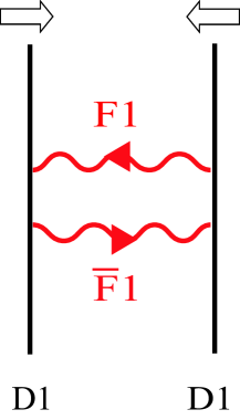
If we consider the classical dynamics of the thin BPS D-vortices in the $(x,y)$-plane, the pair production of fundamental string (F1) and anti-fundamental string (${\overline{\rm F}1}$) as shown in Fig. 2 is neglected for colliding BPS D-strings. Although the zero modes are not identified completely different from multi-BPS Nielsen-Olesen vortices Weinberg:1979er , we assume that the time-dependence of the field naturally appears only in the vortex positions,

$${\bf x}_{p}(t)=(x_{p}(t),y_{p}(t)).$$ (46)

We begin with the tachyon-field configuration in Eqs. (25)–(26),

$$\tau=\lim_{\tau_{{\rm BPS}}\rightarrow\infty}\prod_{p=1}^{n}\tau_{{\rm BPS}}|{\bf x}-{\bf x}_{p}(t)|,\quad\chi=\pm\sum_{p=1}^{n}\tan^{-1}\frac{y-y_{p}(t)}{x-x_{p}(t)},$$ (47)

and the moduli-space dynamics can be described by the time evolution of the vortex positions. Different from the moduli-space dynamics of BPS Nielsen-Olesen vortices with finite thickness Shellard:1988zx , there is a possibility to derive the classical Lagrangian of the $n$ point BPS D-vortices in an exact form from the action (17) by integrating the Lagrangian density over the space,

$${}L({\bf x}_{p}(t),{\dot{\bf x}}_{p}(t)) \equiv \int d^{2}x\lim_{\tau_{{\rm BPS}}\rightarrow\infty}\,{\cal L}(\tau,\chi,\partial_{\mu}\tau,\partial_{\mu}\chi)$$ (48)

$$= -\int d^{2}x\lim_{\tau_{{\rm BPS}}\rightarrow\infty}{\cal H}_{\rm BPS}\sqrt{1+\frac{\tau^{2}\left[-(\partial_{0}\ln\tau)^{2}-(\partial_{0}\chi)^{2}-(\partial_{0}\tau\partial_{i}\chi-\partial_{i}\tau\partial_{0}\chi)^{2}\right]}{\left(1+S_{xx}\right)^{2}}}\,.$$ (49)

The delta-function property (36) results from the energy integration performed in the previous section and will be used in what follows. Using the tachyon profiles in Eq. (47), the derivatives are obtained as

$$\partial_{0}\ln\tau = -\sum_{p=1}^{n}{\dot{\bf x}}_{p}(t)\cdot\frac{\partial\tau}{\partial({\bf x}-{\bf x}_{p}(t))}=-\sum_{p=1}^{n}\frac{{\dot{\bf x}}_{p}(t)\cdot({\bf x}-{\bf x}_{p}(t))}{\left|{\bf x}-{\bf x}_{p}(t)\right|^{2}},\quad\partial_{i}\ln\tau=\sum_{p=1}^{n}\frac{({\bf x}-{\bf x}_{p}(t))^{i}}{\left|{\bf x}-{\bf x}_{p}(t)\right|^{2}},$$ (50)

$$\partial_{0}\chi = -\sum_{p=1}^{n}{\dot{\bf x}}_{p}(t)\cdot\frac{\partial\chi}{\partial({\bf x}-{\bf x}_{p}(t))}=\sum_{p=1}^{n}\frac{\epsilon_{ij}{\dot{\bf x}_{p}^{i}}\,({\bf x}-{\bf x}_{p}(t))^{j}}{\left|{\bf x}-{\bf x}_{p}(t)\right|^{2}},\quad\partial_{i}\chi=-\sum_{p=1}^{n}\frac{\epsilon_{ij}({\bf x}-{\bf x}_{p}(t))^{j}}{\left|{\bf x}-{\bf x}_{p}(t)\right|^{2}}.$$ (51)

Plugging these derivatives into Eq. (49) and using the expression of the Hamiltonian density (35) in terms of the tachyon profiles, we have

$$L({\bf x}_{p}(t),{\dot{\bf x}}_{p}(t)) = -{\cal T}_{0}\int d^{2}x\sum_{s_{1}=1}^{n}\delta^{(2)}({\bf x}-{\bf x}_{s_{1}})$$ (52)

$$\times \lim_{\tau_{{\rm BPS}}\rightarrow\infty}\sqrt{1-\frac{\displaystyle{\left(\prod_{s_{2}=1}^{n}\tau_{{\rm BPS}}|{\bf x}-{\bf x}_{s_{2}}|\right)^{2}\sum_{p,q=1}^{n}\frac{\cos\theta_{pq}}{\tau_{{\rm BPS}}|{\bf x}-{\bf x}_{p}|\tau_{{\rm BPS}}|{\bf x}-{\bf x}_{q}|}}}{\displaystyle{\frac{1}{\tau_{{\rm BPS}}^{2}}+\left(\prod_{s_{3}=1}^{n}\tau_{{\rm BPS}}|{\bf x}-{\bf x}_{s_{3}}|\right)^{2}\sum_{s_{4},s_{5}=1}^{n}\frac{\cos\theta_{s_{4}s_{5}}}{\tau_{{\rm BPS}}|{\bf x}-{\bf x}_{s_{4}}|\tau_{{\rm BPS}}|{\bf x}-{\bf x}_{s_{5}}|}}}{\,\dot{\bf x}}_{p}\cdot{\dot{\bf x}}_{q}}\;.$$

Performing the delta-function integration and taking the $\tau_{{\rm BPS}}\rightarrow\infty$ limit, we obtain the expected result

$$L({\bf x}_{p}(t),{\dot{\bf x}}_{p}(t))=-{\cal T}_{0}\sum_{p=1}^{n}\sqrt{1-{\dot{\bf x}}_{p}^{2}}\,.$$ (53)

This Lagrangian describes $n$ relativistic free particles of mass ${\cal T}_{0}$ in the speed limit $|{\dot{\bf x}}_{p}|\leq 1$ and outside the range of mutual interaction. It correctly reflects the character of point-like classical BPS D-vortices of which actual dynamics is governed by the relativistic field equation of a complex tachyon $T(t,{\bf x})$ and the gauge fields of U(1)$\times$U(1) symmetry. In addition, since the size of the BPS D-vortex is zero, the free Lagrangian description (53) is valid for any case of small separation between two D-vortices. The relativistic Lagrangian (48) of multi-BPS objects has never been derived through systematic studies of moduli-space dynamics.

Figure 3: Scattering picture of (a) BPS Nielsen-Olesen vortices and (b) two identical BPS D-vortices. Since the two vortices are identical, a vortex sees only the half space (the shaded region is equivalent to the unshaded region). In addition, there is a ${\rm Z}_{2}$ symmetry between the upper and the lower quadrant. After semi-diametric dashed lines are identified, the moduli space for a vortex becomes a cone. For the finite-size Nielsen-Olesen vortices, the moduli space is a stubbed cone, and there is only the 90^∘ scattering. For the zero-size D-vortices, the moduli space is a sharp cone. Considering the symmetry the scattering has two possibilities, 90^∘ scattering and 0^∘ (equivalently 180^∘) scattering.

Figure 4: Scattering picture of two identical BPS D-strings for (a) reconnection (corresponding to 90^∘ scattering of D-vortices) and (b) passing through (corresponding to $0^{\circ}$/180^∘ scattering of D-vortices). In the figures, the arrow on the string represents the signature of vorticity, and the arrows perpendicular to the string represent the direction of motion. In the two figures on the right, the arrows for D-vortex scattering in Fig. 3-(b) are presented. In all of the four figures, the scattering points and their trajectories before collision are marked as red for both strings since they are identical. In (a), the trajectories of D-vortices after $90^{\circ}$ scattering are given by the blue lines. The reconnection of D-strings is possible only for pairs of ${\rm A}$-${\rm B}$ and ${\rm C}$-${\rm D}$ since the other pairs of reconnection is not allowed considering the vorticity. In (b), the trajectories after $0^{\circ}$ and $180^{\circ}$ scattering are given by the green lines, both of which lead to the passing through of two identical BPS D-strings.

The methods of the moduli-space dynamics of multi-BPS vortices with the canonical form of kinetic term assume a slow motion of BPS solitons, and then read the metric of moduli space Shellard:1988zx ; MS . Therefore, its relativistic regime is supplemented only by numerical analysis which solves field equations directly. The relativistic Lagrangian (48) obtained here is free from perturbative open string degrees due to the decay of unstable D${\bar{\rm D}}$. It means that the classical dynamics of BPS D-vortices with nonzero separation can be safely described by Eq. (48), and thus by Eq. (53), and is consistent with the numerical analysis dealing with time-dependent field equations. One may also ask whether or not this relativistic Lagrangian of free particles is a consequence of the DBI type action. The specific question is how much the square-root form of the DBI action (17) plays a role in derivation. Although we do not have any other example to compare, the Lagrangian (48) supports the validity of the DBI-type action (17) as a tree-level Lagrangian.

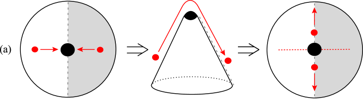
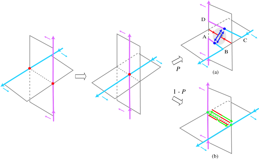
The results of D-vortices in our model describe the parallel D-strings obtained from the coincidence limit of D3${\bar{\rm D}}$3. Finally we consider the collision of two identical BPS D-vortices in Ref. Cho:2007jf . The classical dynamics of cosmic D-strings can be read off from our results. For a collision of two Nielson-Olesen vortices, one vortex sees only a half of the space since the two vortices are identical. The resulting moduli space becomes, therefore, a cone with a stubbed apex due to the finite size of the vortex. The geodesic motion in this moduli space is overcoming the apex straightly, which corresponds to the right-angle scattering in the physical space Shellard:1988zx . (See the red lines in Fig. 3-(a).) Applied to crossing cosmic strings, this right-angle scattering results in the reconnection of the strings after scattering. (See the Fig. 4-(a).) This is the only possible motion for Nielsen-Olesen cosmic strings, and the reconnection probability is always one, $P=1$ Shellard:1988ki .

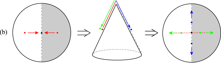
For the identical BPS D-vortices, in addition to the right-angle scattering (see the blue lines in Fig. 3-(b)), there also exist $0^{\circ}$ (passing-through) and $180^{\circ}$ scattering motions (see the green lines in Fig. 3-(b)) which are indistinguishable. Since the BPS D-vortices are thin, the moduli geometry is a cone with a sharp singular apex. The motion at the tip of the cone is then unpredictable, and what we can apply is only the symmetry argument; the vortex motion is either overcoming the tip or bouncing back there. The bouncing-back motion of D-vortices in the moduli space corresponds to the $0^{\circ}$ or $180^{\circ}$ scattering of two identical cosmic D-strings crossing in the physical space. (See Fig. 4-(b).) This affects the reconnection probability of cosmic superstrings and one has $P<1$. This classical result with the help of a quantum concept of identical particles predicts only the possible scattering patterns. The probability $P$ is determined by taking into account the quantum correction as shown in Fig. 2.

V Conclusions

In this work, we obtained the BPS solution to the multi D-vortices produced in the coincidence limit of D2${\bar{\rm D}}$2. The model is described by a DBI-type action with a complex tachyon field. With a gaussian type-potential, we showed that the BPS limit is achieved by an infinitely thin tachyon profile. The obtained BPS configuration correctly reproduces the BPS sum rule and descent relation which result in the identification of BPS D-vortices as BPS D-branes of codimension two.

For multi BPS D-vortices, it is expected that the thin vortices are point-like particles moving freely when they are separated. Assuming that the time-dependence of the system is encoded only in the vortex positions in dynamics, we integrated the Lagrangian of the DBI action to obtain a simple Lagrangian $L^{(n)}({\bf x}_{p},{\dot{\bf x}}_{p})=-{\cal T}_{0}\sum_{p=1}^{n}\sqrt{1-{\dot{\bf x}}_{p}^{2}}$ which describes $n$ free relativistic point particles with the mass given by the D0-brane tension.

While the scattering of Nielsen-Olesen vortices exhibits only the 90^∘ scattering, the scattering of BPS D-vortices exhibits also the $0^{\circ}$/180^∘ scattering. When this scattering picture is applied to the interaction of cosmic superstrings, it implies that two identical BPS D-strings can pass through each other ($0^{\circ}$/180^∘ scattering) as well as can reconnect (90^∘ scattering). This is one of the key differences of cosmic superstrings from usual cosmic strings.