The Organization of Intrinsic Computation:
Complexity-Entropy Diagrams and
the Diversity of Natural Information Processing

Abstract

Intrinsic computation refers to how dynamical systems store, structure, and transform historical and spatial information. By graphing a measure of structural complexity against a measure of randomness, complexity-entropy diagrams display the range and different kinds of intrinsic computation across an entire class of system. Here, we use complexity-entropy diagrams to analyze intrinsic computation in a broad array of deterministic nonlinear and linear stochastic processes, including maps of the interval, cellular automata and Ising spin systems in one and two dimensions, Markov chains, and probabilistic minimal finite-state machines. Since complexity-entropy diagrams are a function only of observed configurations, they can be used to compare systems without reference to system coordinates or parameters. It has been known for some time that in special cases complexity-entropy diagrams reveal that high degrees of information processing are associated with phase transitions in the underlying process space, the so-called “edge of chaos”. Generally, though, complexity-entropy diagrams differ substantially in character, demonstrating a genuine diversity of distinct kinds of intrinsic computation.

Discovering organization in the natural world is one of science’s central goals. Recent innovations in nonlinear mathematics and physics, in concert with analyses of how dynamical systems store and process information, has produced a growing body of results on quantitative ways to measure natural organization. These efforts had their origin in earlier investigations of the origins of randomness. Eventually, however, it was realized that measures of randomness do not capture the property of organization. This led to the recent efforts to develop measures that are, on the one hand, as generally applicable as the randomness measures but which, on the other, capture a system’s complexity—its organization, structure, memory, regularity, symmetry, and pattern. Here—analyzing processes from dynamical systems, statistical mechanics, stochastic processes, and automata theory—we show that measures of structural complexity are a necessary and useful complement to describing natural systems only in terms of their randomness. The result is a broad appreciation of the kinds of information processing embedded in nonlinear systems. This, in turn, suggests new physical substrates to harness for future developments of novel forms of computation.

I Introduction

The past several decades have produced a growing body of work on ways to measure the organization of natural systems. (For early work, see, e.g., Refs. [1, 2, 3, 4, 5, 6, 7, 8, 9, 10, 11, 12, 13, 14, 15, 16, 17, 18, 19, 20]; for more recent reviews, see Refs. [21, 22, 23, 24, 25, 26, 27, 28].) The original interest derived from explorations, during the 60’s to the mid-80’s, of behavior generated by nonlinear dynamical systems. The thread that focused especially on pattern and structural complexity originated, in effect, in attempts to reconstruct geometry [29], topology [30], equations of motion [31], periodic orbits [32], and stochastic processes [33] from observations of nonlinear processes. More recently, developing and using measures of complexity has been a concern of researchers studying neural computation [34, 35], the clinical analysis of patterns from a variety of medical signals and imaging technologies [36, 37, 38], and machine learning and synchronization [39, 40, 41, 42, 43], to mention only a few contemporary applications.

These efforts, however, have their origin in an earlier period in which the central concern was not the emergence of organization, but rather the origins of randomness. Specifically, measures were developed and refined that quantify the degree of randomness and unpredictability generated by dynamical systems. These quantities—metric entropy, Lyapunov characteristic exponents, fractal dimensions, and so on—now provide an often-used and well understood set of tools for detecting and quantifying deterministic chaos of various kinds. In the arena of stochastic processes, Shannon’s entropy rate predates even these and has been productively used for half a century as a measure of an information source’s degree of randomness or unpredictability [44].

Over this long early history, researchers came to appreciate that dynamical systems were capable of an astonishing array of behaviors that could not be meaningfully summarized by the entropy rate or fractal dimension. The reason for this is that, by their definition, these measures of randomness do not capture the property of organization. This realization led to the considerable contemporary efforts just cited to develop measures that are as generally applicable as the randomness measures but that capture a system’s complexity—its organization, structure, memory, regularity, symmetry, pattern, and so on.

Complexity measures which do this are often referred to as statistical or structural complexities to indicate that they capture a property distinct from randomness. In contrast, deterministic complexities—such as the Shannon entropy rate, Lyapunov characteristic exponents, and the Kolmogorov-Chaitin complexity—are maximized for random systems. In essence, they are simply alternatives to measuring the same property—degrees of randomness. Here, we shall emphasize complexity of the structural and statistical sort which measures a property complementary to randomness. We will demonstrate, across a broad range of model systems, that measures of structural complexity are a necessary and useful addition to describing a process in terms of its randomness.

I.1 Structural Complexity

How might one go about developing a structural complexity measure? A typical starting point is to argue that that the structural complexity of a system must reach a maximum between the system’s perfectly ordered and perfectly disordered extremes [45, 5, 6, 15, 14, 19, 9, 46]. The basic idea behind these claims is that a system which is either perfectly predictable (e.g., a periodic sequence) or perfectly unpredictable (e.g., a fair coin toss) is deemed to have zero structural complexity. Thus, the argument goes, a system with either zero entropy or maximal entropy (usually normalized to one), has zero complexity; these systems are simple and not highly structured. This line of reasoning further posits that in between these extremes lies complexity. Those objects that we intuitively consider to be complex must involve a continuous element of newness or novelty (i.e., entropy), but not to such an extent that the novelty becomes completely unpredictable and degenerates into mere noise.

In summary, then, it is common practice to require that a structural complexity measure vanish in the perfectly ordered and perfectly disordered limits. Between these limits, the complexity is usually assumed to achieve a maximum. These requirements are often taken as axioms from which one constructs a complexity measure that is a single-valued function of randomness as measured by, say, entropy. In both technical and popular scientific literatures, it is not uncommon to find a “complexity” plotted against entropy in merely schematic form as a sketch of a generic complexity function that vanishes for extreme values of entropy and achieves a maximum in a middle region [5, 47, 48, 49]. Several authors, in fact, have taken these as the only constraints defining complexity [50, 51, 52, 53, 54].

Here we take a different approach: We do not prescribe how complexity depends on entropy. One reason for this is that a useful complexity measure needs to do more than satisfy the boundary conditions of vanishing in the high- and low-entropy limits [24, 55, 56]. In particular, a useful complexity measure should have an unambiguous interpretation that accounts in some direct way for how correlations are organized in a system. To that end we consider a well defined and frequently used complexity measures—the excess entropy—and empirically examine its relationship to entropy for a variety of systems.

I.2 Complexity-Entropy Diagrams

The diagnostic tool that will be the focal point for our studies is the complexity-entropy diagram. Introduced in Ref. [14], a complexity-entropy diagram plots structural complexity (vertical axis) versus randomness (horizontal axis) for systems in a given model class. Complexity-entropy diagrams allow for a direct view of the complexity-entropy relationship within and across different systems. For example, one can easily read whether or not complexity is a single-valued function of entropy.

The complexity and entropy measures that we use capture a system’s intrinsic computation [19]: how a system stores, organizes, and transforms information. A crucial point is that these measures of intrinsic computation are properties of the system’s configurations. They do not require knowledge of the equations of motion or Hamiltonian or of system parameters (e.g., temperature, dissipation, or spin-coupling strength) that generated the configurations. Hence, in addition to the many cases in which they can be calculated analytically, they can be inductively calculated from observations of symbolic sequences or configurations.

Thus, a complexity-entropy diagram measures intrinsic computation in a parameter-free way. This allows for the direct comparison of intrinsic computation across very different classes since a complexity-entropy diagram expresses this in terms of common “information-processing” coordinates. As such, a complexity-entropy diagram demonstrates how much a given resource (e.g., stored information) is required to produce a given amount of randomness (entropy), or how much novelty (entropy) is needed to produce a certain amount of statistical complexity.

Recently, a form of complexity-entropy diagram has been used in the study of anatomical MRI brain images [38, 57]. This work showed that complexity-entropy diagrams give a reliable way to distinguish between “normal” brains and those experiencing cortical thinning, a condition associated with Alzheimer’s disease. Complexity-entropy diagrams have also recently been used as part of a proposed test to distinguish chaos from noise [58]. And Ref. [59] calculates complexity-entropy diagrams for a handful of different complexity measures using the sequences generated by the symbolic dynamics of various chaotic maps.

Historically, one of the motivations behind complexity-entropy diagrams was to explore the common claim that complexity achieves a sharp maximum at a well defined boundary between the order-disorder extremes. This led, for example, to the widely popularized notion of the “edge of chaos” [60, 61, 62, 63, 64, 65, 66, 67]—namely, that objects achieve maximum complexity at a boundary between order and disorder. Although these particular claims have been criticized [68], during the same period it was shown that at the onset of chaos complexity does reach a maximum. Specifically, Ref. [14] showed that the statistical complexity diverges at the accumulation point of the period-doubling route to chaos. This led to an analytical theory that describes exactly the interdependence of complexity and entropy for this universal route to chaos [16]. Similarly, another complexity measure, the excess entropy [1, 2, 6, 12, 18, 27, 69, 70, 71] has also been shown to diverge at the period-doubling critical point.

This latter work gave some hope that there would be a universal relationship between complexity and entropy—that some appropriately defined measure of complexity plotted against an appropriate entropy would have the same functional form for a wide variety of systems. In part, the motivation for this was the remarkable success of scaling and data collapse for critical phenomena. Data collapse is a phenomena in which certain variables for very different systems collapse onto a single curve when appropriately rescaled near the critical point of a continuous phase transition. For example, the magnetization and susceptibility exhibit data collapse near the ferromagnet-paramagnet transition. See, for example, Refs. [72, 73] for further discussion. Data collapse reveals that different systems—e.g., different materials with different critical temperatures—possess a deep similarity despite differences in their details.

The hope, then, was to find a similar universal curve for complexity as a function of entropy. One now sees that this is not and, fortunately, cannot be the case. Notwithstanding special parametrized examples, such as period-doubling and other routes to chaos, a wide range of complexity-entropy relationships exists [19, 18, 74, 24]. This is a point that we will repeatedly reinforce in the following.

I.3 Surveying Complexity-Entropy Diagrams

We will present a survey of the relationships between structure and randomness for a number of familiar, well studied systems including deterministic nonlinear and linear stochastic processes and well known models of computation. The systems we study include maps of the interval, cellular automata and Ising models in one and two dimensions, Markov chains, and minimal finite-state machines. To our knowledge, this is the first such cross-model survey of complexity-entropy diagrams.

The main conclusion that emerges from our results is that there is a large range of possible complexity-entropy behaviors. Specifically, there is not a universal complexity-entropy curve, there is not a general complexity-entropy transition, nor is it case that complexity-entropy diagrams for different systems are even qualitatively similar. These results give a concrete picture of the very different types of relationship between a system’s rate of information production and the structural organization which produces that randomness. This diversity opens up a number of interesting mathematical questions, and it appears to suggest a new kind of richness in nature’s organization of intrinsic computation.

Our exploration of intrinsic computation is structured as follows: In Section II we briefly review several information-theoretic quantities, most notably the entropy rate and the excess entropy. In Section III we present results for the complexity-entropy diagrams for a wide range of model systems. In Section IV we discuss our results, make a number of general comments and observations, and conclude by summarizing.

II Entropy and Complexity Measures

II.1 Information-Theoretic Quantities

The complexity-entropy diagrams we will examine make use of two information-theoretic quantities: the excess entropy and the entropy rate. In this section we fix notation and give a brief but self-contained review of them.

We begin by describing the stochastic process generated by a system. Specifically, we are interested here in describing the character of bi-infinite, one-dimensional sequences: $\stackrel{{\scriptstyle\leftrightarrow}}{{S}}=\ldots,S_{-2},S_{-1},S_{0},S_{1},\ldots$, where the $S_{i}$’s are random variables that assume values $s_{i}$ in a finite alphabet $\mathcal{A}$. Throughout, we follow the standard convention that a lower-case letter refers to a particular value of the random variable denoted by the corresponding upper-case letter. In the following, the index $i$ on the $S_{i}$’s will refer to either space or time.

A process is, quite simply, the distribution over all possible sequences generated by a system: ${\rm P}(\stackrel{{\scriptstyle\leftrightarrow}}{{S}})$. Let ${\rm P}(s_{i}^{L})$ denote the probability that a block $S_{i}^{L}=S_{i}S_{i+1}\ldots S_{i+L-1}$ of $L$ consecutive symbols takes on the particular values $s_{i},s_{i+1},\ldots,s_{i+L-1}\in\mathcal{A}$. We will assume that the distribution over blocks is stationary: ${\rm P}(S_{i}^{L})={\rm P}(S_{i+M}^{L})$ for all $i$, $M$, and $L$. And so we will drop the index on the block probabilities. When there is no confusion, then, we denote by $s^{L}$ a particular sequence of $L$ symbols, and use ${\rm P}(s^{L})$ to denote the probability that the particular $L$-block occurs.

The support of a process is the set of allowed sequences—i.e., those with positive probability. In the parlance of computation theory, a process’ support is a formal language: the set of all finite length words that occur at least once in an infinite sequence.

A special class of processes that we will consider in subsequent sections are Order-$R$ Markov Chains. These processes are those for which the joint distribution can be conditionally factored into words $S^{R}$ of length $R$—that is,

$${\rm P}(\stackrel{{\scriptstyle\leftrightarrow}}{{S}})=\ldots{\rm P}(S_{i}^{R}|S_{i-R}^{R}){\rm P}(S_{i+R}^{R}|S_{i}^{R}){\rm P}(S_{i+2R}^{R}|S_{i+R}^{R})\ldots\;.$$ (1)

In other words, knowledge of the current length-$R$ word is all that is needed to determine the distribution of future symbols. As a result, the states of the Markov chain are associated with the $\mathcal{A}^{R}$ possible values that can be assumed by a length-$R$ word.

We now briefly review several central quantities of information theory that we will use to develop measures of unpredictability and entropy. For details see any textbook on information theory; e.g., Ref. [44]. Let $X$ be a random variable that assumes the values $x\in{\cal X}$, where ${\cal X}$ is a finite set. The probability that $X$ assumes the value $x$ is given by ${\rm P}(x)$. Also, let $Y$ be a random variable that assumes values $y\in{\cal Y}$.

The Shannon entropy of the variable $X$ is given by:

$$H[X]\,\equiv\,-\sum_{x\in{\cal X}}{\rm P}(x)\log_{2}{\rm P}(x)\;.$$ (2)

The units are given in bits. This quantity measures the uncertainty associated with the random variable $X$. Equivalently, $H[X]$ is also the average amount of memory needed to store outcomes of variable $X$.

The joint entropy of two random variables, X and Y, is defined as:

$$H[X,Y]\,\equiv\,-\sum_{x\in{\cal X},y\in{\cal Y}}{\rm P}(x,y)\log_{2}{\rm P}(x,y)\;.$$ (3)

It is a measure of the uncertainty associated with the joint distribution ${\rm P}(X,Y)$. The conditional entropy is defined as:

$$H[X|Y]\,\equiv\,-\sum_{x\in{\cal X},y\in{\cal Y}}{\rm P}(x,y)\log_{2}{\rm P}(x|y)\;,$$ (4)

and gives the average uncertainty of the conditional probability ${\rm P}(X|Y)$. That is, $H[X|Y]$ tells us how uncertain, on average, we are about $X$, given that the outcome of $Y$ is known.

Finally, the mutual information is defined as:

$$I[X;Y]\,\equiv\,H[X]-H[X|Y]\;.$$ (5)

It measures the average reduction of uncertainty of one variable due to knowledge of another. If knowing $Y$ on average reduces uncertainty about $X$, then it makes sense to say that $Y$ carries information about $X$. Note that $I[X;Y]=I[Y;X]$.

II.2 Entropy Growth and Entropy Rate

With these definitions set, we are ready to develop an information-theoretic measure of a process’s randomness. Our starting point is to consider blocks of consecutive variables. The block entropy is the total Shannon entropy of length-$L$ sequences:

$$H(L)\,\equiv\,-\sum_{s^{L}\in{\cal A}^{L}}{\rm P}(s^{L})\log_{2}{\rm P}(s^{L})\;,$$ (6)

where $L>0$. The sums run over all possible blocks of length $L$. We define $H(0)\equiv 0$. The block entropy grows monotonically with block length: $H(L)\geq H(L-1)$.

For stationary processes the total Shannon entropy typically grows linearly with $L$. That is, for sufficiently large $L$, $H(L)\sim L$. This leads one to define the entropy rate ${h_{\mu}}$ as:

$${h_{\mu}}\,\equiv\,\lim_{L\rightarrow\infty}\frac{H(L)}{L}\;.$$ (7)

The units of ${h_{\mu}}$ are bits per symbol. This limit exists for all stationary sequences [44, Chapter 4.2]. The entropy rate is also know as the metric entropy in dynamical systems theory and is equivalent to the thermodynamic entropy density familiar from equilibrium statistical mechanics.

The entropy rate can be given an additional interpretation as follows. First, we define an $L$-dependent entropy rate estimate:

$${h_{\mu}}(L) \,=\, H(L)-H(L\!-\!1)$$ (8)

$$\,=\, H[S_{L}|S_{L-1},S_{L-2},\ldots,S_{1}]\;,\;\;L>0\;.$$ (9)

We set ${h_{\mu}}(0)=\log_{2}|{\cal A}|$. In words, then, ${h_{\mu}}(L)$ is the average uncertainty of the next variable $S_{L}$, given that the previous $L\!-\!1$ symbols have been seen. Geometrically, $h_{\mu}(L)$ is the two-point slope of the total entropy growth curve $H(L)$. Since conditioning on more variables can never increase the entropy, it follows that ${h_{\mu}}(L)\leq{h_{\mu}}(L-1)$. In the $L\rightarrow\infty$ limit, ${h_{\mu}}(L)$ is equal to the entropy rate defined above in Eq. (7):

$${h_{\mu}}\,=\,\lim_{L\rightarrow\infty}{h_{\mu}}(L)\;.$$ (10)

Again, this limit exists for all stationary processes [44]. Equation (10) tells us that ${h_{\mu}}$ may be viewed as the irreducible randomness in a process—the randomness that persists even after statistics over longer and longer blocks of variables are taken into account.

II.3 Excess Entropy

The entropy rate gives a reliable and well understood measure of the randomness or disorder intrinsic to a process. However, as the introduction noted, this tells us little about the underlying system’s organization, structure, or correlations. Looking at the manner in which ${h_{\mu}}(L)$ converges to its asymptotic value ${h_{\mu}}$, however, provides one measure of these properties.

When observations only over length-$L$ blocks are taken into account, a process appears to have an entropy rate of ${h_{\mu}}(L)$. This quantity is larger than the true, asymptotic value of the entropy rate ${h_{\mu}}$. As a result, the process appears more random by ${h_{\mu}}(L)-{h_{\mu}}$ bits. Summing these entropy over-estimates over $L$, one obtains the excess entropy [1, 2, 6, 12]:

$${\bf E}\,\equiv\,\sum_{L=1}^{\infty}[{h_{\mu}}(L)-{h_{\mu}}]\;.$$ (11)

The units of ${\bf E}$ are bits. The excess entropy tells us how much information must be gained before it is possible to infer the actual per-symbol randomness ${h_{\mu}}$. It is large if the system possesses many regularities or correlations that manifest themselves only at large scales. As such, the excess entropy can serve as a measure of global structure or correlation present in the system.

This interpretation is strengthened by noting that the excess entropy can also be expressed as the mutual information between two adjacent semi-infinite blocks of variables [18, 27]:

$${\bf E}\,=\,\lim_{L\rightarrow\infty}I[S_{-L},S_{-L+1},S_{-1};S_{0},S_{1},\ldots S_{L-1}]\;.$$ (12)

Thus, the excess entropy measures one type of the memory of the system; it tells us how much knowledge of one half of the system reduces our uncertainty about the other half. If the sequence of random variables is a time series, then ${\bf E}$ is the amount of information the past shares with the future.

The excess entropy may also be given a geometric interpretation. The existence of the entropy rate suggests that $H(L)$ grows linearly with $L$ for large $L$ and that the growth rate, or slope, is given by ${h_{\mu}}$. It is then possible to show that the excess entropy is the “$y$-intercept” of the asymptotic form for $H(L)$ [2, 6, 18, 75, 39, 40]:

$$H(L)\,\sim\,{\bf E}+{h_{\mu}}L~{},\;{\rm as}\;L\rightarrow\infty\;.$$ (13)

Or, rearranging, we have

$${\bf E}\,=\,\lim_{L\rightarrow\infty}\left[H(L)-{h_{\mu}}L\right]\;.$$ (14)

This form of the excess entropy highlights another interpretation: ${\bf E}$ is the cost of amnesia. If an observer has extracted enough information from a system (at large $L$) to predict it optimally ($\sim{h_{\mu}}$), but suddenly loses all of that information, the process will then appear more random by an amount $H(L)-{h_{\mu}}L$.

To close, note that the excess entropy, originally coined in [1], goes by a number of different names, including “stored information” [2]; “effective measure complexity” [6, 12, 76, 8, 77]; “complexity” [18, 75]; “predictive information” [39, 40]; and “reduced Rényi entropy of order $1$” [78, 79]. For recent reviews on excess entropy, entropy convergence in general, and applications of this approach see Refs. [22, 27, 39].

II.4 Intrinsic Information Processing Coordinates

In the model classes examined below, we shall take the excess entropy ${\bf E}$ as our measure of complexity and use the entropy rate ${h_{\mu}}$ as the randomness measure. The excess entropy ${\bf E}$ and the entropy rate ${h_{\mu}}$ are exactly the two quantities that specify the large-$L$ asymptotic form for the block entropy Eq. (13). The set of all $({h_{\mu}},{\bf E})$ pairs is thus geometrically equivalent to the set of all straight lines with non-negative slope and intercept. Clearly, a line’s slope and intercept are independent quantities. Thus, there is no a priori reason to anticipate any relationship between ${h_{\mu}}$ and ${\bf E}$, a point emphasized early on by Li [18].

It is helpful in the following to know that for binary order-$R$ Markov processes there is an upper bound on the excess entropy:

$${\bf E}\leq R(1-h_{\mu})\;.$$ (15)

We sketch a justification of this result here; for the derivation, see [27, Proposition 11]. First, recall that the excess entropy may be written as the mutual information between two semi-infinite blocks, as indicated in Eq. (12). However, given the process is order-$R$ Markovian, Eq. (1), the excess entropy reduces to the mutual information between two adjacent $R$-blocks. From Eq. (5), we see that the excess entropy is the entropy of an $R$-block minus the entropy of an $R$-block conditioned on its neighboring $R$-block:

$${\bf E}\,=\,H(R)-H[S_{i}^{R}|S_{i-R}^{R}]\;.$$ (16)

(Note that this only holds in the special case of order-$R$ Markov processes. It is not true in general.) The first term on the right hand side of Eq. (16) is maximized when the distribution over the $R$-block is uniform, in which case $H(R)=R$. The second term on the right hand side is minimized by assuming that the conditional entropy of the two blocks is given simply by $Rh_{\mu}$—i.e., $R$ times the per-symbol entropy rate $h_{\mu}$. In other words, we obtain a lower bound by assuming that the process is independent, identically distributed over $R$-blocks. Combining the two bounds gives Eq. (15).

It is also helpful in the following to know that for periodic processes ${h_{\mu}}=0$ (perfectly predictable) and ${\bf E}=\log_{2}p$, where $p$ is the period [27]. In this case, ${\bf E}$ is the amount of information required to distinguish the $p$ phases of the cycle.

II.5 Calculating Complexities and Entropies

As is now clear, all quantities of interest depend on knowing sequence probabilities ${\rm P}(s^{L})$. These can be obtained by direct analytical approximation given a model or by numerical estimation via simulation. Sometimes, in special cases, the complexity and entropy can be calculated in closed form.

For some, but not all, of the process classes studied in the following, we estimate the various information-theoretic quantities by simulation. We generate a long sequence, keeping track of the frequency of occurrence of words up to some finite length $L$. The word counts are stored in a dynamically generated parse tree, allowing us to go out to $L=120$ in some cases. We first make a rough estimate of the topological entropy using a small $L$ value. This entropy determines the sparseness of the parse tree, which in turn determines how large a tree can be stored in a given amount of memory. From the word and subword frequencies ${\rm P}(s^{L})$, one directly calculates $H(L)$ and, thus, ${h_{\mu}}$ and ${\bf E}$. Estimation errors in these quantities are a function of statistical errors in ${\rm P}(s^{L})$.

Here, we are mainly interested in gaining a general sense of the behavior of the entropy rate ${h_{\mu}}$ and the excess entropy ${\bf E}$. And so, for the purposes of our survey, this direct method is sufficient. The vast majority of our estimates are accurate to at least $1\%$. If extremely accurate estimates are needed, there exist a variety of techniques for correcting for estimator bias [80, 81, 82, 83, 84, 85]. When one is working with finite data, there is also the question of what errors occur, since the $L\rightarrow\infty$ limit cannot be taken. For more on this issue, see Ref. [27].

Regardless of these potential subtleties, the entropy rate and excess entropy can be reliably estimated via simulation, given access to a reasonably large amount of data. Moreover, this estimation is purely inductive—one does not need to use knowledge of the underlying equations of motion or the hidden states that produced the sequence. Nevertheless, for several of the model classes we consider—one-dimensional Ising models, Markov chains, and topological Markov chains—we calculate the quantities using closed-form expressions, leading to essentially no error.

III Complexity-Entropy Diagrams

In the following sections we present a survey of intrinsic computation across a wide range of process classes. We think of a class of system as given by equations of motion, or other specification for a stochastic process, that are parametrized in some way—a pair of control parameters in a one-dimensional map or the energy of a Hamiltonian, say. The space of parameters, then, is the concrete representation of the space of possible systems, and a class of system is a subset of the set of all possible processes. A point in the parameter space is then a particular system, whose intrinsic computation we will summarize by a pair of numbers—one a measure of randomness, the other a measure of structure. In several cases, these measures are estimated from sequences generated by the temporal or spatial process.

III.1 One-Dimensional Discrete Iterated Maps

Here we look at the symbolic dynamics generated by two iterated maps of the interval—the well studied logistic and tent maps—of the form:

$$x_{n+1}=f_{\mu}(x_{n})~{},$$ (17)

where $\mu$ is a parameter that controls the nonlinear function $f$, $x_{n}\in[0,1]$, and one starts with $x_{0}$, the initial condition. The logistic and tent maps are canonical examples of systems exhibiting deterministic chaos. The nonlinear iterated function $f$ consists of two monotone pieces. And so, one can analyze the maps’ behavior on the interval via a generating partition that reduces a sequence of continuous states $x_{0},x_{1},x_{2},\ldots$ to a binary sequence $s_{0},s_{1},s_{2},\ldots$ [86]. The binary partition is given by

$$s_{i}=\left\{\begin{array}[]{cl}0&x\leq\frac{1}{2}\\ \\ 1&x>\frac{1}{2}\end{array}\right.~{}.$$ (18)

The binary sequence may be viewed as a code for the set of initial conditions that produce the sequence. When the maps are chaotic, arbitrarily long binary sequences produced using this partition code for arbitrarily small intervals of initial conditions on the chaotic attractor. Hence, one can explore many of these maps’ properties via binary sequences.

III.1.1 Logistic Map

We begin with the logistic map of the unit interval:

$$f(x)\,=\,rx(1-x)\;,$$ (19)

where the control parameter $r\in[0,4]$. We iterate this starting with an arbitrary initial condition $x_{0}\in[0,1]$. In Fig. 1 we show numerical estimates of the excess entropy ${\bf E}$ and the entropy rate ${h_{\mu}}$ as a function of $r$. Notice that both ${\bf E}$ and ${h_{\mu}}$ change in a complicated matter as the parameter $r$ is varied continuously.

As $r$ increases from $3.0$ to approximately $3.5926$, the logistic map undergoes a series of period-doubling bifurcations. For $r\in(3.0,3.2361)$ the sequences generated by the logistic map are periodic with period two, for $r\in(3.2361,3.4986)$ the sequences are period 4, and for $r\in(3.4986,3.5546)$ the sequences are period $8$. For all periodic sequences of period $p$, the entropy rate ${h_{\mu}}$ is zero and the excess entropy ${\bf E}$ is $\log_{2}p$. So, as the period doubles, the excess entropy increases by one bit. This can be seen in the staircase on the left hand side of Fig. 1. At $r\approx 3.5926$, the logistic map becomes chaotic, as evidenced by a positive entropy rate. For further discussion of the phenomenology of the logistic map, see almost any modern textbook on nonlinear dynamics, e.g., Refs. [87, 88].

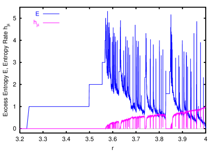
Figure 1: Excess entropy ${\bf E}$ and entropy rate ${h_{\mu}}$ as a function of the parameter $r$. The top curve is excess entropy. The $r$ values were sampled uniformly as $r$ was varied from $3.4$ to $4.0$ in increments of $0.0001$. The largest $L$ used was $L=30$ for systems with low entropy. For each parameter value with positive entropy, $1\times 10^{7}$ words of length $L$ were sampled.

Looking at Fig. 1, it is difficult to see how ${\bf E}$ and $h_{\mu}$ are related. This relationship can be seen much more clearly in Fig. 2, in which we show the complexity-entropy diagram for the same system. That is, we plot $({h_{\mu}},{\bf E})$ pairs. This lets us look at how the excess entropy and the entropy rate are related, independent of the parameter $r$.

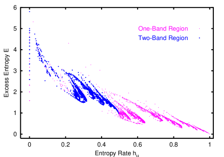
Figure 2: Entropy rate and excess entropy $({h_{\mu}},{\bf E})$-pairs for logistic map. Points from regions of the map in which the bifurcation diagram has one or two bands are colored differently. There are $3214$ parameter values sampled for the one-band region and $3440$ values for the two-band region. The $r$ values were sampled uniformly. The one-band region is $r\in(3.6786,4.0)$; the two-band region is $r\in(3.5926,3.6786)$. The largest $L$ used was $L=30$ for systems with low entropy. For each parameter value with positive entropy, $1\times 10^{7}$ words of length $L$ were sampled.

Figure 2 shows that there is a definite relationship between ${\bf E}$ and ${h_{\mu}}$—one that is not immediately evident from looking at Fig. 1. Note, however, that this relationship is not a simple one. In particular, complexity is not a function of entropy: ${\bf E}\neq g({h_{\mu}})$. For a given value of ${h_{\mu}}$, multiple excess entropy values ${\bf E}$ are possible.

There are several additional empirical observations to extract from Fig. 2. First, the shape appears to be self-similar. This is not at all surprising, given that the logistic map’s bifurcation diagram itself is self-similar. Second, note the clumpy, nonuniform clustering of $({h_{\mu}},{\bf E})$ pairs within the dense region. Third, note that there is a fairly well defined lower bound. Fourth, for a given value of the entropy rate $h_{\mu}$ there are many possible values for the excess entropy ${\bf E}$. However, it appears as if not all ${\bf E}$ values are possible for a given $h_{\mu}$. Lastly, note that there does not appear to be any phase transition (at finite $h_{\mu}$) in the complexity-entropy diagram. Strictly speaking, such a transition does occur, but it does so at zero entropy rate. As the period doublings accumulate, the excess entropy grows without bound. As a result, the possible excess entropy values at $h_{\mu}=0$ on the complexity-entropy diagram are unbounded. For further discussion, see Ref. [16].

III.1.2 Tent Map

We next consider the tent map:

$$f(x)\,=\,\left\{\begin{array}[]{ll}ax&x<\frac{1}{2}\\ \\ \hskip 2.84526pta(1-x)&x\geq\frac{1}{2}\end{array}\right.\;,$$ (20)

where $a\in[0,2]$ is the control parameter. For $a\in[1,2]$, the entropy rate ${h_{\mu}}=\log_{2}a$; when $a\in[0,1]$, ${h_{\mu}}=0$. Fig. 3 shows $1,200$ $({h_{\mu}},{\bf E})$-pairs in which ${\bf E}$ is calculated numerically from empirical estimates of the binary word distribution ${\rm P}(s^{L})$.

Figure 3: Excess entropy ${\bf E}$ versus entropy density ${h_{\mu}}$ for the tent map. The $L$ used to estimate ${\rm P}(s^{L})$, and so ${\bf E}$ and ${h_{\mu}}$, varied depending on the $a$ parameter. The largest $L$ used was $L=120$ at low ${h_{\mu}}$. The plot shows $1,200$ $({h_{\mu}},{\bf E})$-pairs. The parameter was incremented every $\Delta a=5\times 10^{-4}$ for $a\in[1,1.2]$ and then incremented every $\Delta a=0.001$ for $a\in[1.2,2.0]$. For each parameter value with positive entropy, $10^{7}$ words of length $L$ were sampled.

Reference [16] developed a phenomenological theory that explains the properties of the tent map at the so-called band-merging points, where bands of the chaotic attractor merge pairwise as a function of the control parameter. The behavior at these points is noisy periodic—the order of band visitations is periodic, but motion within is deterministic chaotic. They occur when $a=2^{2^{-n}}$. The symbolic-dynamic process is described by a Markov chain consisting of a periodic cycle of $2^{n}$ states in which all state-to-state transitions are nonbranching except for one where $s_{i}=0$ or $s_{i}=1$ with equal probability. Thus, each phase of the Markov chain has zero entropy per transition, except for the one that has a branching entropy of $1$ bit. The entropy rate at band-mergings is thus ${h_{\mu}}=2^{-n}$, with $n$ an integer.

The excess entropy for the symbolic-dynamic process at the $2^{n}$-to-$2^{n-1}$ band-merging is simply ${\bf E}=\log_{2}2^{n}=n$. That is, the process carries $n$ bits of phase information. Putting these facts together, then, we have a very simple relationship in the complexity-entropy diagram at band-mergings:

$${\bf E}\,=\,-\log_{2}{h_{\mu}}~{}.$$ (21)

This is graphed as the dashed line in Fig. 3. It is clear that the entire complexity-entropy diagram is much richer than this simple expression indicates. Nonetheless, Eq. (21) does capture the overall shape quite well.

Note that, in sharp contrast to the logistic map, for the tent map it does appear as if the excess entropy takes on only a single value for each value of the entropy rate ${h_{\mu}}$. The reason for this is straightforward. The entropy rate ${h_{\mu}}$ is a simple monotonic function of the parameter $a$—$h_{\mu}=\log_{2}a$—and so there is a one-to-one relationship between them. As a result, each $h_{\mu}$ value on the complexity-entropy diagram corresponds to one and only one value of $a$ and, in turn, corresponds to one and only one value of ${\bf E}$. Interestingly, the excess entropy appears to be a continuous function of $h_{\mu}$, although not a differentiable one.

III.2 Ising Spin Systems

We now investigate the complexity-entropy diagrams of the Ising model in one and two spatial dimensions. Ising models are among the simplest physical models of spatially extended systems. Originally introduced to model magnetic materials, they are now used to model a wide range of cooperative phenomena and order-disorder transitions and, more generally, are viewed as generic models of spatially extended, statistical mechanical systems [89, 90]. Like the logistic and tent maps, Ising models are also studied as an intrinsically interesting mathematical topic. As we will see, Ising models provide an interesting contrast with the intrinsic computation seen in the interval maps.

Specifically, we consider spin-$1/2$ Ising models with nearest (NN) and next-nearest neighbor (NNN) interactions. The Hamiltonian (energy function) for such a system is:

$${\cal H}\, = \,-J_{1}\sum_{\langle i,j\rangle_{\rm nn}}S_{i}S_{j}$$ (22)

$$-J_{2}\sum_{\langle i,j\rangle_{{\rm nnn}}}S_{i}S_{j}\,-\,B\sum_{i}S_{i}\;,$$

where the first (second) sum is understood to run over all NN (NNN) pairs of spins. In one dimension, a spin’s nearest-neighbors will consist of two spins, one to the right and one to the left, whereas in two dimensions a spin will have four nearest neighbors—left, right, up, and down. Each spin $S_{i}$ is a binary variable: $S_{i}\,\in\,\{-1,+1\}$. The coupling constant $J_{1}$ is a parameter that when positive (negative) makes it energetically favorable for NN spins to (anti-)align. The constant $J_{2}$ has the same effect on NNN spins. The parameter $B$ may be viewed as an external field; its effect is to make it energetically favorable for spins to point up (i.e., have a value of $+1$) instead of down. The probability of a configuration is taken to be proportional to its Boltzmann weight: the probability of a spin configuration ${\cal C}$ is proportional to $e^{-\beta{\cal H}({\cal C})}$, where $\beta=1/T$ is the inverse temperature.

In equilibrium statistical mechanics, the entropy density is a monotonic increasing function of the temperature. Quite generically, a plot of the entropy $h_{\mu}$ as a function of temperature $T$ resembles that of the top plot in Fig. 6. Thus, $h_{\mu}$ may be viewed as a nonlinearly rescaled temperature. One might ask, then, why one might want to plot complexity versus entropy: Isn’t a plot of complexity versus temperature qualitatively the same? Indeed, the two plots would look very similar. However, there are two major benefits of complexity-entropy diagrams for statistical mechanical systems. First, the entropy captures directly the system’s unpredictability, measured in bits per spin. The entropy thus measures the system’s information processing properties. Second, plotting complexity versus entropy and not temperature allows for a direct comparison of the range of information processing properties of statistical mechanical systems with systems for which there is not a well defined temperature, such as the deterministic dynamical systems of the previous section or the cellular automata of the subsequent one.

III.2.1 One-Dimensional Ising System

We begin by examining one-dimensional Ising systems. In Refs. [74, 25, 91] two of the authors developed exact, analytic transfer-matrix methods for calculating ${h_{\mu}}$ and ${\bf E}$ in the thermodynamic ($N\rightarrow\infty$) limit. These methods make use of the fact the NNN Ising model is order-$2$ Markovian. We used these methods to produce Fig. 4, the complexity-entropy diagram for the NNN Ising system with antiferromagnetic coupling constants $J_{1}$ and $J_{2}$ that tend to anti-align coupled spins. The figure gives a scatter plot of $10^{5}$ $({h_{\mu}},{\bf E})$ pairs for system parameters that were sampled randomly from the following ranges: $J_{1}\in[-8,0]$, $J_{2}\in[-8,0]$, $T\in[0.05,6.05]$, and $B\in[0,3]$. For each parameter realization, the excess entropy ${\bf E}$ and entropy density ${h_{\mu}}$ were calculated. Fig. 4 is rather striking—the $({h_{\mu}},{\bf E})$ pairs are organized in the shape of a “batcape”. Why does the plot have this form?

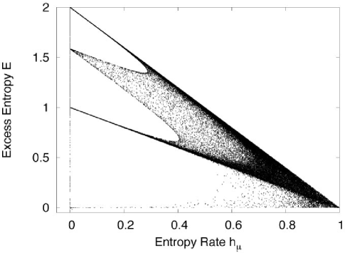
Figure 4: Complexity-entropy diagram for the one-dimensional, spin-$1/2$ antiferromagnetic Ising model with nearest- and next-nearest-neighbor interactions. $10^{5}$ system parameters were sampled randomly from the following ranges: $J_{1}\in[-8,0]$, $J_{2}\in[-8,0]$, $T\in[0.05,6.05]$, and $B\in[0,3]$. For each parameter setting, the excess entropy ${\bf E}$ and entropy density ${h_{\mu}}$ were calculated analytically.

Recall that if a sequence over a binary alphabet is periodic with period $p$, then ${\bf E}=\log_{2}p$ and ${h_{\mu}}=0$. Thus, the “tips” of the batcape at ${h_{\mu}}=0$ correspond to crystalline (periodic) spin configurations with periods $1$, $2$, $3$, and $4$. For example, the $(0,0)$ point is the period-$1$ configuration with all spins aligned. These periodic regimes correspond to the system’s different possible ground states. As the entropy density increases, the cape tips widen and eventually join.

Figure 4 demonstrates in graphical form that there is organization in the process space defined by the Hamiltonian of Eq. (22). Specifically, for antiferromagnetic couplings, ${\bf E}$ and ${h_{\mu}}$ values do not uniformly fill the plane. There are forbidden regions in the complexity-entropy plane. Adding randomness (${h_{\mu}}$) to the periodic ground states does not immediately destroy them. That is, there are low-entropy states that are almost-periodic. The apparent upper linear bound is that of Eq. (15) for a system with at most $4$ Markov states or, equivalently, a order-$2$ Markov chain: ${\bf E}\leq 2-2{h_{\mu}}$.

In contrast, in the logistic map’s complexity-entropy diagram (Fig. 2) one does not see anything remotely like the batcape. This indicates that there are no low-entropy, almost-periodic configurations related to the exactly periodic configurations generated at zero-entropy along the period-doubling route to chaos. Increasing the parameter there does not add randomness to a periodic orbit. Rather, it causes a system bifurcation to a higher-period orbit.

III.2.2 Two-Dimensional Ising Model

Thus far we have considered only one-dimensional systems, either temporal or spatial. However, the excess entropy can be extended to apply to two-dimensional configurations as well; for details, see Ref. [92]. Using methods from there, we calculated the excess entropy and entropy density for the two-dimensional Ising model with nearest- and next-nearest-neighbor interactions. In other words, we calculated the complexity-entropy diagram for the two-dimensional version of the system whose complexity-entropy diagram is shown in Fig. 4. There are several different definitions for the excess entropy in two dimensions, all of which are similar but not identical. In Fig. 4 we used a version that is based on the mutual information and, hence, is denoted ${{\bf E}}_{I}$ [92].

Figure 5 gives a scatter plot of $4,500$ complexity-entropy pairs. System parameters in Eq. (22) were sampled randomly from the following ranges: $J_{1}\in[-3,0]$, $J_{2}\in[-3,0]$, $T\in[0.05,4.05]$, and $B=0$. For each parameter setting, the excess entropy ${\bf E}_{I}$ and entropy density ${h_{\mu}}$ were estimated numerically; the configurations themselves were generated via a Monte Carlo simulation. For each $({h_{\mu}},{\bf E})$ point the simulation was run for $200,000$ Monte Carlo updates per site to equilibrate. Configuration data was then taken for $20,000$ Monte Carlo updates per site. The lattice size was a square of $48\times 48$ spins. The long equilibration time is necessary because, for some Ising models at low temperature, single-spin flip dynamics of the sort used here have very long transient times [93, 94, 95].

Note the similarity between Figs. 4 and 5. For the 2D model, there is also a near-linear upper bound: ${\bf E}\leq 5(1-h_{\mu})$. In addition, one sees periodic spin configurations, as evidenced by the horizontal bands. An ${\bf E}_{I}$ of $1$ bit corresponds to a checkerboard of period $2$; ${\bf E}_{I}=3$ corresponds to a checkerboard of period $4$; while ${\bf E}_{I}=2$ corresponds to a “staircase” pattern of period $4$. See Ref. [92] for illustrations. The two period-$4$ configurations are both ground states for the model in the parameter regime in which $|J_{2}|<|J_{1}|$ and $J_{2}<0$. At low temperatures, the state into which the system settles is a matter of chance.

Figure 5: Complexity-entropy diagram for the two-dimensional, spin-$1/2$ antiferromagnetic Ising model with nearest- and next-nearest-neighbor interactions. System parameters were sampled randomly from the following ranges: $J_{1}\in[-3,0]$, $J_{2}\in[-3,0]$, $T\in[0.05,4.05]$, and $B=0$. For each parameter setting, the excess entropy ${\bf E}_{I}$ and entropy density ${h_{\mu}}$ were estimated numerically.

Thus, the horizontal streaks in the low-entropy region of Fig. 5 are the different ground states possible for the system. In this regard Fig. 5 is qualitatively similar to Fig. 4—in each there are several possible ground states at ${h_{\mu}}=0$ that persist as the entropy density is increased. However, in the two-dimensional system of Fig. 5 one sees a scatter of other values around the periodic bands. There are even ${\bf E}_{I}$ values larger than $3$. These ${\bf E}_{I}$ values arise when parameters are selected in which the NN and NNN coupling strengths are similar; $J_{1}\approx J_{2}$. When this is the case, there is no energy cost associated with a horizontal or vertical defect between the two possible ground states. As a result, for low temperatures the systems effectively freezes into horizontal or vertical strips consisting of the different ground states. Depending on the number of strips and their relative widths, a number of different ${\bf E}_{I}$ values are possible, including values well above $3$, indicating very complex spatial structure.

Despite these differences, the similarities between the complexity-entropy plots for the one- and two-dimensional systems is clearly evident. This is all the more noteworthy since one- and two-dimensional Ising models are regarded as very different sorts of system by those who focus solely on phase transitions. The two-dimensional Ising model has a critical phase transition while the one-dimensional does not. And, more generally, two-dimensional random fields are generally considered very different mathematical entities than one-dimensional sequences. Nevertheless, the two complexity-entropy diagrams show that, away from criticality, the one- and two-dimensional Ising systems’ ranges of intrinsic computation are similar.

III.2.3 Ising Model Phase Transition

As noted above, the two-dimensional Ising model is well known as a canonical model of a system that undergoes a continuous phase transition—a discontinuous change in the system’s properties as a parameter is continuously varied. The 2D NN Ising model with ferromagnetic ($J_{1}>0$) bonds and no NNN coupling ($J_{2}=0$) and zero external field ($B=0$) undergoes a phase transition at $T=T_{c}\approx 2.269$ when $J_{1}=1$. At the critical temperature $T_{c}$ the magnetic susceptibility diverges and the specific heat is not differentiable. In Fig. 5 we restricted ourselves to antiferromagnetic couplings and thus did not sample in the region of parameter space in which the phase transition occurs.

What happens if we fix $J_{1}=1$, $J_{2}=0$, and $B=0$, and vary the temperature? In this case, we see that the complexity, as measured by ${\bf E}$, shows a sharp maximum near the critical temperature $T_{c}$. Figure 6 shows results obtained via a Monte Carlo simulation on a $100\times 100$ lattice. We used a Wolff cluster algorithm and periodic boundary conditions. After $10^{6}$ Monte Carlo steps (one step is one proposed cluster flip), $25,000$ configurations were sampled, with $200$ Monte Carlo steps between measurements. This process was repeated for over $200$ samples between $T=0$ and $T=6$. More temperatures were sampled near the critical region.

Figure 6: Entropy rate vs. temperature, excess entropy vs. temperature, and the complexity-entropy diagram for the 2D NN ferromagnetic Ising model. Monte Carlo results for $200$ temperatures between $0$ and $6$. The temperature was sampled more densely near the critical temperature. For further discussion, see text.

In Fig. 6 we first plot entropy density ${h_{\mu}}$ and excess entropy ${\bf E}$ versus temperature. As expected, the excess entropy reaches a maximum at the critical temperature $T_{c}$. At $T_{c}$ the correlations in the system decay algebraically, whereas they decay exponentially for all other $T_{c}$ values. Hence, ${\bf E}$, which may be viewed as a global measure of correlation, is maximized at $T_{c}$. For the system of Fig. 6, $T_{c}$ appears to have an approximate value of $2.42$. This is above the exact value for an infinite system, which is $T_{c}\approx 2.27$. Our estimated value is higher, as one expects for a finite lattice. At the critical temperature, $h_{\mu}\approx 0.57$, and ${\bf E}\approx 0.413$.

Also in Fig. 6 we show the complexity-entropy diagram for the 2D Ising model. This complexity-entropy diagram is a single curve, instead of the scatter plots seen in the previous complexity-entropy diagrams. The reason is that we varied a single parameter, the temperature, and entropy is a single-valued function of the temperature, as can clearly be seen in the first plot in Fig. 6. Hence, there is only one value of ${h_{\mu}}$ for each temperature, leading to a single curve for the complexity-entropy diagram.

Note that the peak in the complexity-entropy diagram for the 2D Ising model is rather rounded, whereas ${\bf E}$ plotted versus temperature shows a much sharper peak. The reason for this rounding is that the entropy density ${h_{\mu}}$ changes very rapidly near $T_{c}$. The effect is to smooth the ${\bf E}$ curve when plotted against ${h_{\mu}}$.

A similar complexity-entropy was produced by Arnold [75]. He also estimated the excess entropy, but did so by considering only one-dimensional sequences of measurements obtained at a single site, while a Monte Carlo simulation generated a sequence of two-dimensional configurations. Thus, those results do not account for two-dimensional structure but, rather, reflect properties of the dynamics of the particular Monte Carlo updating algorithm used. Nevertheless, the results of Ref. [75] are qualitatively similar to ours.

Erb and Ay [96] have calculated the multi-information for the two-dimensional Ising model as a function of temperature. The multi-information is the difference between the entropy rate and the entropy of a single site: $H(1)-h_{\mu}$. That is, the multi-information is only the leading term in the sum which defines the excess entropy, Eq. (11). (Recall that $h_{\mu}(1)=H(1)$.) They find that the multi-information is a continuous function of the temperature and that it reaches a sharp peak at the critical temperature [96, Fig. 4].

III.3 Cellular Automata

The next process class we consider is cellular automata (CAs) in one and two spatial dimensions. Like spin systems, CAs are common prototypes used to model spatially extended dynamical systems. For reviews see, e.g., Refs. [97, 98, 99]. Unlike the Ising models of the previous section, the CAs that we study here are deterministic. There is no noise or temperature in the system.

The states of the CAs we shall consider consist of one- or two-dimensional configurations ${\mathbf{s}}=\ldots s^{-1},s^{0},s^{1},\ldots$ of discrete $K$-ary local states $s^{i}\in\{0,1,\ldots,K-1\}$. The configurations change in time according to a global update function $\mathbf{\Phi}$:

$${\mathbf{s}}_{t+1}^{i}={\mathbf{\Phi}}{\mathbf{s}}_{t}^{i}~{},$$ (23)

starting from an initial configuration ${\mathbf{s}}_{0}$. What makes CAs cellular is that configurations evolve according to a local update rule. The value $s_{t+1}^{i}$ of site $i$ at the next time step is a function $\phi$ of the site’s previous value and the values of neighboring sites within some radius $r$:

$$s_{t+1}^{i}=\phi(s_{t}^{i-r}\ldots,s_{t}^{i}\ldots,s_{t}^{i+r})~{}.$$ (24)

All sites are updated synchronously. The CA update rule $\phi$ consists of specifying the output value $s_{t+1}$ for all possible neighborhood configurations $\eta_{t}=s_{t}^{i-r}\ldots,s_{t}^{i}\ldots,s_{t}^{i+r}$. Thus, for 1D radius-$r$ CAs, there are $K^{2r+1}$ possible neighborhood configurations and $2^{K^{2r+1}}$ possible CA rules. The $r=1$, $K=2$ 1D CAs are called elementary cellular automata [97].

In all CA simulations reported we began with an arbitrary random initial configuration ${\mathbf{s}}_{0}$ and iterated the CA several thousand times to let transient behavior die away. Configuration statistics were then accumulated for an additional period of thousands of time steps, as appropriate. Periodic boundary conditions on the underlying lattice were used.

In Fig. 7 we show the results of calculating various complexity-entropy diagrams for 1D, $r=2$, $K=2$ (binary) cellular automata. There are $2^{2^{5}}\approx 4.3\times 10^{9}$ such CAs. We cannot examine all $4.3$ billion CAs; instead we sample the space these CAs uniformly. For the data of Fig. 7, the lattice has $5\times 10^{4}$ sites and a transient time of $5\times 10^{4}$ iterations was used. We plot ${h_{\mu}}$ versus ${\bf E}$ for spatial sequences. Plots for the temporal sequences are qualitatively similar. There are several things to observe in these diagrams.

Figure 7: Spatial entropy density $h^{s}_{\mu}$ and spatial excess entropy ${\bf E}^{s}$ for a random sampling of $10^{3}$ $r=2$, binary 1D CAs.

One feature to notice in Fig. 7 is that no sharp peak in the excess entropy appears at some intermediate ${h_{\mu}}$ value. In contrast, the maximum possible excess entropy falls off moderately rapidly with increasing ${h_{\mu}}$. A linear upper bound, ${\bf E}\leq 4(1-h_{\mu})$, is almost completely respected. Note that, as is the case with the other complexity-entropy diagrams presented here, for all ${h_{\mu}}$ values except ${h_{\mu}}=1$, there is a range of possible excess entropies.

In the early 1990’s there was considerable exploration of the organization of CA rule space. In particular, a series of papers [62, 100, 101, 102] looked at two-dimensional eight-state ($K=8$) cellular automata, with a neighborhood size of $5$ sites—the site itself and its nearest neighbor to the north, east, west, and south. These references reported evidence for the existence of a phase transition in the complexity-entropy diagram at a critical entropy level. In contrast, however, here and in the previous sections we find no evidence for such a transition. The reasons that Refs. [62, 100, 101, 102] report a transition are two-fold. First, they used very restricted measures of randomness and complexity: entropy of single isolated sites and mutual information of neighboring pairs of single sites, respectively. These choices have the effect of projecting organization onto their complexity-entropy diagrams. The organization seen is largely a reflection of constraints on the chosen measures, not of intrinsic properties of the CAs. Second, they do not sample the space of CA’s uniformly; rather, they parametrize the space of CAs and sample only by sweeping their single parameter. This results in a sample of CA space that is very different from uniform and that is biased toward higher complexity CAs. For a further discussion of complexity-entropy diagrams for cellular automata, including a discussion of Refs. [62, 100, 101, 102], see Ref. [103].

III.4 Markov Chain Processes

In this and the next section, we consider two classes of process that provide a basis of comparison for the preceding nonlinear dynamics and statistical mechanical systems: those generated by Markov chains and topological $\epsilon$-machines. These classes are complementary to each other in the following sense. Topological $\epsilon$-machines represent structure in terms of which sequences (or configurations) are allowed or not. When we explore the space of topological $\epsilon$-machines, the associated processes differ in which sets of sequences occur and which are forbidden. In contrast, when exploring Markov chains, we fix a set of allowed words—in the present case the full set of binary sequences—and then vary the probability with which subwords occur. These two classes thus represent two different types of possible organization in intrinsic computation—types that were mixed in the preceding example systems.

In Fig. 8 we plot ${\bf E}$ versus ${h_{\mu}}$ for order-$2$ ($4$-state) Markov chains over a binary alphabet. Each element in the stochastic transition matrix $T$ is chosen uniformly from the unit interval. The elements of the matrix are then normalized row by row so that $\sum_{j}T_{ij}=1$. We generated $10^{5}$ such matrices and formed the complexity-entropy diagram shown in Fig. 8. Since these processes are order-$2$ Markov chains, the bound of Eq. (15) applies. This bound is the sharp, linear upper limit evident in Fig. 8: ${\bf E}\,=2-2{h_{\mu}}$.

It is illustrative to compare the $4$-state Markov chains considered here with the 1D NNN Ising models of Sec. III.2.1. The order-$2$ (or $4$-state Markov) chains with a binary alphabet are those systems for which the value of a site depends on the previous two sites, but no others. In terms of spin systems, then, this is a spin-$1/2$ (i.e., binary) system with nearest- and next-nearest neighbors. The transition matrix for the Markov chain is $4\times 4$ and thus has $16$ elements. However, since each row of the transition matrix must be normalized, there are $12$ independent parameters for this model class. In contrast, there are only $3$ independent parameters for the 1D NNN Ising chain—the parameters $J_{1}$, $J_{2}$, $B$, and the temperature $T$. One of the parameters may be viewed as setting an energy scale, so only three are independent.

Thus, the 1D NNN systems are a proper subset of the $4$-state Markov chains. Note that their complexity-entropy diagrams are very different, as a quick glance at Figs. 4 and 8 confirms. The reason for this is that the Ising model, due to its parametrization (via the Hamiltonian of Eq. (22)), samples the space of processes in a very different way than the Markov chains. This underscores the crucial role played by the choice of model and, so too, the choice in parametrizing a model space. Different parametrizations of the same model class, when sampled uniformly over those parameters, yield complexity-entropy diagrams with different structural properties.

Figure 8: Excess-entropy, entropy-rate pairs for $10^{5}$ randomly selected $4$-state Markov chains.

III.5 The Space of Processes: Topological $\epsilon$-Machines

The preceding model classes are familiar from dynamical systems theory, statistical mechanics, and stochastic process theory. Each has served an historical purpose in their respective fields—purposes that reflect mathematically, physically, or statistically useful parametrizations of the space of processes. In the preceding sections we explored these classes, asked what sort of processes they could generate, and then calculated complexity-entropy pairs for each process to reveal the range of possible information processing within each class.

Is there a way, though, to directly explore the space of processes, without assuming a particular model class or parametrization? Can each process be taken at face value and tell us how it is structured? More to the point, can we avoid making structural assumptions, as done in the preceding sections?

Affirmative answers to these questions are found in the approach laid out by computational mechanics [14, 19, 28]. Computational mechanics demonstrates that each process has an optimal, minimal, and unique representation—the $\epsilon$-machine—that captures the process’s structure. Due to optimality, minimality, and uniqueness, the $\epsilon$-machine may be viewed as the representation of its associated process. In this sense, this representation is parameter free. To determine an $\epsilon$-machine for a process one calculates a set of causal states and their transitions. In other words, one does not specify a priori the number of states or the transition structure between them. Determining the $\epsilon$-machine makes such no structural assumptions [19, 28].

Using the one-to-one relationship between processes and their $\epsilon$-machines, here we invert the preceding logic of going from a process to its $\epsilon$-machine. We explore the space of processes by systematically enumerating $\epsilon$-machines and then calculating their excess entropies ${\bf E}$ and their entropy rates $h_{\mu}$. This gives a direct view of how intrinsic computation is organized in the space of processes.

As a complement to the Markov chain exploration of how intrinsic computation depends on transition probability variation, here we examine how an $\epsilon$-machine’s structure (states and their connectivity) affects information processing. We do this by restricting attention to the class of topological $\epsilon$-machines whose branching transition probabilities are fair (equally probable). (An example is shown in Fig. 10.)

If we regard two $\epsilon$-machines isomorphic up to variation in transition probabilities as members of a single equivalence class, then each such class of $\epsilon$-machines contains precisely one topological $\epsilon$-machine. (Symbolic dynamics [104] refers to a related class of representations as topological Markov chains. An essential, and important, difference is that $\epsilon$-machines always have the smallest number of states.)

Causal States	Topological
n	$\epsilon$-machines
1	3
2	7
3	78
4	1,388
5	35,186

Table 1: The number of topological binary $\epsilon$-machines up to $n=5$ causal states. (After Ref. [105].)

It turns out that the topological $\epsilon$-machines with a finite number of states can be systematically enumerated [105]. Here we consider only $\epsilon$-machines for binary processes: $\mathcal{A}=\{0,1\}$. Two $\epsilon$-machines are isomorphic and generate essentially the same stochastic process, if they are related by a relabeling of states or if their output symbols are exchanged: $0$ is mapped to $1$ and vice versa. The number of isomorphically distinct topological $\epsilon$-machines of $n=1,\ldots,5$ states is listed in Table 1.

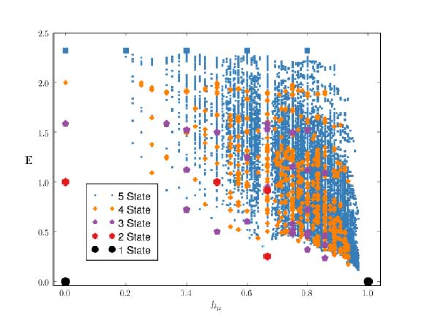
Figure 9: Complexity-entropy pairs $(h_{\mu},{\bf E})$ for all topological binary $\epsilon$-machines with $n=1,\ldots,4$ states and for $35,041$ of the $35,186$ $5$-state $\epsilon$-machines. The excess entropy is estimated as ${\bf E}(L)=H(L)-L{h_{\mu}}$ using the exact value for the entropy rate ${h_{\mu}}$ and a storage-efficient type-class algorithm [106] for the block entropy $H(L)$. The estimates were made by increasing $L$ until ${\bf E}(L)-{\bf E}(L-1)<\delta$, where $\delta=0.0001$ for $1$, $2$, and $3$ states; $\delta=0.0050$ for $4$ states; and $\delta=0.0100$ for 5 states.

In Fig. 9 we plot their $({h_{\mu}},{\bf E})$ pairs. There one sees that the complexity-entropy diagram exhibits quite a bit of organization, with variations from very low to very high density of $\epsilon$-machines co-existing with several distinct vertical (iso-entropy) families. To better understand the structure in the complexity-entropy diagram, though, it is helpful to consider bounds on the complexities and entropies of Fig. 9. The minimum complexity, ${\bf E}=0$, corresponds to machines with only a single state. There are two possibilities for such binary $\epsilon$-machines. Either they generate all $1$s (or $0$s) or all sequences occurring with equal probability (at each length). If the latter, then ${h_{\mu}}=1$; if the former, ${h_{\mu}}=0$. These two points, $(0,0)$ and $(1,0)$, are denoted with solid circles along Fig. 9’s horizontal axis.

Figure 10: An example topological $\epsilon$-machine for a cyclic process in $\mathcal{F}_{5,3}$. Note that branching occurs only between pairs of successive states in the cyclic chain. The excess entropy for this process is $\log_{2}5\approx 2.32$, and the entropy rate is $3/5$.

The maximum ${\bf E}$ in the complexity-entropy diagram is $\log_{2}5\approx 2.3219$. One such $\epsilon$-machine corresponds to the zero-entropy, period-$5$ processes. And there are four similar processes with periods $p=1,2,3,4$ at the points $(0,\log_{2}p)$. These are denoted on the figure by the tokens along the left vertical axis.

There are other period-$5$ cyclic, partially random processes with maximal complexity, though; those with causal states in a cyclic chain. These have $b=1,2,3,4$ branching transitions between successive states in the chain and so positive entropy. These appear as a horizontal line of enlarged square tokens along in the upper portion of the complexity-entropy diagram. Denote the family of $p$-cyclic processes with $b$ branchings as $\mathcal{F}_{p,b}$. An $\epsilon$-machine illustrating $\mathcal{F}_{5,3}$ is shown in Fig. 10. The excess entropy for this process is $\log_{2}5\approx 2.32$, and the entropy rate is $3/5$.

Since $\epsilon$-machines for cyclic processes consist of states in a single loop, their excess entropies provide an upper bound among $\epsilon$-machines that generate $p$-cyclic processes with $b$ branchings states, namely:

$${\bf E}(\mathcal{F}_{p,b})=\log_{2}(p)~{}.$$ (25)

Clearly, ${\bf E}(\mathcal{F}_{p,b})\rightarrow\infty$ as $p\rightarrow\infty$. Their entropy rates are given by a similarly simple expression:

$${h_{\mu}}(\mathcal{F}_{p,b})=\frac{b}{p}~{}.$$ (26)

Note that ${h_{\mu}}(\mathcal{F}_{p,b})\rightarrow 0$ as $p\rightarrow\infty$ with fixed $b$ and ${h_{\mu}}(\mathcal{F}_{p,b})\rightarrow 1$ as $b\rightarrow p$. Together, then, the family $\mathcal{F}_{5,b}$ gives an upper bound to the complexity-entropy diagram.

The processes $\mathcal{F}_{p,b}$ are representatives of the highest points of the prominent jutting vertical towers of $\epsilon$-machines so prevalent in Fig. 9. It therefore seems reasonable to expect the $({h_{\mu}},{\bf E})$ coordinates for $p$-cyclic process languages to possess at least $p-1$ vertical towers, distributed evenly at ${h_{\mu}}=b/p$, $b=1,\dots,p-1$, and for these towers to correspond with towers of $m$-cyclic process languages whenever $m$ is a multiple of $p$.

These upper bounds are one key difference from earlier classes in which there was a decreasing linear upper bound on complexity as a function of entropy rate: ${\bf E}\leq R(1-h_{\mu})$. That is, in the space of processes, many are not so constrained. The subspace of topological $\epsilon$-machines illustrates that there are many highly entropic, highly structured processes. Some of the more familiar model classes appear to inherit, in their implied parametrization of process space, a bias away from such processes.

It is easy to see that the families $\mathcal{F}_{p,p-1}$ and $\mathcal{F}_{p,1}$ provide upper and lower bounds for ${h_{\mu}}$, respectively, among the process languages that achieve maximal ${\bf E}$ and for which ${h_{\mu}}>0$. Indeed, the smallest positive ${h_{\mu}}$ possible is achieved when only a single of the equally probable states has more than one outgoing transition.

More can be said about this picture of the space of intrinsic computation spanned by topological $\epsilon$-machines [105]. Here, however, our aim is to illustrate how rich the diversity of intrinsic computation can be and to do so independent of conventional model-class parametrizations. These results allow us to probe in a systematic way a subset of processes in which structure dominates.

IV Discussion and Conclusion

Complexity-entropy diagrams provide a common view of the intrinsic information processing embedded in different processes. We used them to compare markedly different systems: one-dimensional maps of the unit interval; one- and two-dimensional Ising models; cellular automata; Markov chains; and topological $\epsilon$-machines. The exploration of each class turned different knobs in the sense that we adjusted different parameters: temperature, nonlinearity, coupling strength, cellular automaton rule, and transition probabilities. Moreover, these parameters had very different effects. Changing the temperature and coupling constants in the Ising models altered the probabilities of configurations, but it did not change which configurations were allowed to occur. In contrast, the topological $\epsilon$-machines exactly expressed what it means for different processes to have different sets of allowed sequences. Changing the CA rules or the nonlinearity parameter in the logistic map combined these effects: the allowed sequences or the probability of sequences or both changed. In this way, the survey illustrated in dramatic fashion one of the benefits of the complexity-entropy diagram: it allows for a common comparison across rather varied systems.

For example, the complexity-entropy diagram for the radius-$2$, one-dimensional cellular automata, shown in Fig. 7, is very different from that of the logistic map, shown in Fig. 2. For the logistic map, there is a distinct lower bound for the excess entropy as a function of the entropy rate. In Fig. 2 this is seen as the large forbidden region at the diagram’s lower portion. In sharp contrast, in Fig. 7 no such forbidden region is seen.

At a more general level of comparison, the survey showed that for a given ${h_{\mu}}$, the excess entropy ${\bf E}$ can be arbitrarily small. This suggests that the intrinsic computation of cellular automata and the logistic map are organized in fundamentally different ways. In turn, the 1D and 2D Ising systems exhibit yet another kind of information processing capability. Each of has well defined ground states—seen as the zero-entropy tips of the “batcapes” in Figs. 4 and 5. These ground states are robust under small amounts of noise—i.e., as the temperature increases from zero. Thus, there are almost-periodic configurations at low entropy. In contrast, there do not appear to be any almost-periodic configurations at low entropy for the logistic map of Fig. 2.

Our last example, topological $\epsilon$-machines, was a rather different kind of model class. In fact, we argued that it gave a direct view into the very structure of the space of processes. In this sense, the complexity-entropy diagram was parameter free. Note, however, that by choosing all branching probabilities to be fair, we intentionally biased this model class toward high-complexity, high-entropy processes. Nevertheless, the distinction between the topological $\epsilon$-machine complexity-entropy diagram of Fig. 9 and the others is striking.

The diversity of possible complexity-entropy diagrams points to their utility as a way to compare information processing across different classes. Complexity-entropy diagrams can be empirically calculated from observed configurations themselves. The organization reflected in the complexity-entropy diagram then provides clues as to an appropriate model class to use for the system at hand. For example, if one found a complexity-entropy diagram with a batcape structure like that of Figs. 4 and 5, this suggests that the class could be well modeled using energies that, in turn, were expressed via a Hamiltonian. Complexity-entropy diagrams may also be of use in classifying behavior within a model class. For example, as noted above, a type of complexity-entropy diagram has already been successfully used to distinguish between different types of structure in anatomical MRI images of brains [38, 57].

Ultimately, the main conclusion to draw from this survey is that there is a large diversity of complexity-entropy diagrams. There is certainly not a universal complexity-entropy curve, as once hoped. Nor is it the case that there are even qualitative similarities among complexity-entropy diagrams. They capture distinctive structure in the intrinsic information processing capabilities of a class of processes. This diversity is not a negative result. Rather, it indicates the utility of this type of intrinsic computation analysis, and it optimistically points to the richness of information processing available in the mathematical and natural worlds. Simply put, information processing is too complex to be simply universal.

References

- [1] J. P. Crutchfield and N. H. Packard. Symbolic dynamics of noisy chaos. Physica D, 7:201–223, 1983.
- [2] R. Shaw. The Dripping Faucet as a Model Chaotic System. Aerial Press, Santa Cruz, California, 1984.
- [3] S. Wolfram. Universality and complexity in cellular automata. Physica, 10D:1–35, 1984.
- [4] C. H. Bennett. On the nature and origin of complexity in discrete, homogeneous locally-interacting systems. Found. Phys., 16:585–592, 1986.
- [5] B. A. Huberman and T. Hogg. Complexity and adaptation. Physica D, 22:376–384, 1986.
- [6] P. Grassberger. Toward a quantitative theory of self-generated complexity. Intl. J. Theo. Phys., 25(9):907–938, 1986.
- [7] P. Szépfalusy and G. Györgyi. Entropy decay as a measure of stochasticity in chaotic systems. Phys. Rev. A, 33(4):2852–2855, 1986.
- [8] K. E. Eriksson and K. Lindgren. Structural information in self-organizing systems. Physica Scripta, 1987.
- [9] M. Koppel. Complexity, depth, and sophistication. Complex Systems, 1:1087–1091, 1987.
- [10] R. Landauer. A simple measure of complexity. Nature, 336(6197):306–307, 1988.
- [11] S. Lloyd and H. Pagels. Complexity as thermodynamic depth. Ann. Physics, 188:186–213, 1988.
- [12] K. Lindgren and M. G. Norhdal. Complexity measures and cellular automata. Complex Systems, 2(4):409–440, 1988.
- [13] P. Szepfalusy. Characterization of chaos and complexity by properties of dynamical entropies. Physica Scripta, T25:226–229, 1989.
- [14] J. P. Crutchfield and K. Young. Inferring statistical complexity. Phys. Rev. Lett., 63:105–108, 1989.
- [15] C. H. Bennett. How to define complexity in physics, and why. In W. H. Zurek, editor, Complexity, Entropy, and the Physics of Information, volume VIII of Santa Fe Institute Studies in the Sciences of Complexity, pages 137–148. Addison-Wesley, 1990.
- [16] J. P. Crutchfield and K. Young. Computation at the onset of chaos. In W. H. Zurek, editor, Complexity, Entropy and the Physics of Information, volume VIII of Santa Fe Institute Studies in the Sciences of Compexity, pages 223–269. Addison-Wesley, 1990.
- [17] R. Badii. Quantitative characterization of complexity and predictability. Phys. Lett. A, 160:372–377, 1991.
- [18] W. Li. On the relationship between complexity and entropy for Markov chains and regular languages. Complex Systems, 5(4):381–399, 1991.
- [19] J. P. Crutchfield. The calculi of emergence: Computation, dynamics, and induction. Physica D, 75:11–54, 1994.
- [20] J. E. Bates and H. K. Shepard. Measuring complexity using information fluctuation. Phys. Lett. A, 172:416–425, 1993.
- [21] B. Wackerbauer, A. Witt, H. Atmanspacher, J. Kurths, and Schein. A comparative classification of complexity measures. Chaos, Solitons & Fractals, 4(1):133–173, 1994.
- [22] W. Ebeling. Prediction and entropy of nonlinear dynamical systems and symbolic sequences with LRO. Physica D, 109:42–52, 1997.
- [23] R. Badii and A. Politi. Complexity: Hierarchical structures and scaling in physics. Cambridge University Press, Cambridge, 1997.
- [24] D. P. Feldman and J. P. Crutchfield. Measures of statistical complexity: Why? Phys. Lett. A, 238:244–252, 1998.
- [25] D. P. Feldman and J. P. Crutchfield. Discovering non-critical organization: Statistical mechanical, information theoretic, and computational views of patterns in simple one-dimensional spin systems. Santa Fe Institute Working Paper 98-04-026, http://hornacek.coa.edu/dave/Publications/DNCO.html.
- [26] I. Nemenman and N. Tishby. Complexity through nonextensivity. Physica A, 302:89–99, 2001.
- [27] J. P. Crutchfield and D. P. Feldman. Regularities unseen, randomness observed: Levels of entropy convergence. Chaos, 15:25–54, 2003.
- [28] C. R. Shalizi and J. P. Crutchfield. Computational mechanics: Pattern and prediction, structure and simplicity. J. Stat. Phys., 104:817–879, 2001.
- [29] N. H. Packard, J. P. Crutchfield, J. D. Farmer, and R. S. Shaw. Geometry from a time series. Phys. Rev. Let., 45, 1980.
- [30] M. R. Muldoon, R. S. Mackay, D. S. Broomhead, and J. Huke. Topology from a time series. Physica D, 65:1–16, 1993.
- [31] J. P. Crutchfield and B. S. Mcnamara. Equations of motion from a data series. Complex Systems, 1, 1987.
- [32] D. Auerbach, P. Cvitanović, J.-P. Eckmann, G. Gunaratne, and I. Procaccia. Exploring chaotic motion through periodic orbits. Physical Review Letters, 58(23):2387+, June 1987.
- [33] A. Fraser. Chaotic data and model building. In H. Atmanspacher and H. Scheingraber, editors, Information Dynamics, volume 256 of NATO ASI Series, pages 125–130. Plenum, 1991.
- [34] G. Tononi, O. Sporns, and G. M. Edelman. A measure for brain complexity: Relating functional segregation and integration in the nervous system. Proceedings of the National Academies of Sciences, 91:5033–5037, 1994.
- [35] T. Wennekers and N. Ay. Finite state automata resulting from temporal information maximization and a temporal learning rule. Neural Comp., 17:2258–2290, 2005.
- [36] P. I. Saparin, W. Gowin, J. Kurths, and D. Felsenberg. Quantification of cencellous bone structure using symbolic dynamics and measures of complexity. Phys. Rev. E, 58:6449–6459, 1998.
- [37] N. Marwan, Meyerfeldt, A. Schirdewan, and J. Kurths. Recurrence-plot-based measures of complexity and their application to heart-rate-variability data. Phys. Rev. E, 66, 2002.
- [38] K. Young, U. Chen, J. Kornak, G. B. Matson, and N. Schuff. Summarizing complexity in high dimensions. Phys. Rev. Lett., 94, 2005.
- [39] W. Bialek, I. Nemenman, and N. Tishby. Predictability, complexity, and learning. Neural Comp., 13:2409–2463, 2001.
- [40] I. Nemenman. Information Theory and Learning: A Physical Approach. PhD thesis, Princeton University, 2000.
- [41] J. P. Crutchfield and D. P. Feldman. Synchronizing to the environment: Information theoretic constraints on agent learning. Adv. Complex Systems, 4:251–264, 2001.
- [42] L. Debowski. Entropic subextensitivity in language and learning. In C. Tsallis and M. Gell-Mann, editors, Nonextensive Entropy: Interdisciplinary Applications, pages 335–345. Oxford University Press, 2004.
- [43] D. P. Feldman and J. P. Crutchfield. Synchronizing to a periodic signal: The transient information and synchronization time of periodic sequences. Adv. Complex Systems, 7:329–355, 2004.
- [44] T. M. Cover and J. A. Thomas. Elements of Information Theory. John Wiley & Sons, Inc., 1991.
- [45] J. P. Crutchfield and N. H. Packard. Symbolic dynamics of one-dimensional maps: Entropies, finite precision, and noise. Intl. J. Theo. Phys., 21:433–466, 1982.
- [46] M. Gell-Mann and S. Lloyd. Information measures, effective complexity, and total information. Complexity, 2(1):44–52, 1996.
- [47] H. Atlan. Les theories de la complexity. In Fogelman F. Soulie, editor, Les Theories de la Complexity. Seuil, Paris, 1991.
- [48] M. Gell-Mann. The Quark and the Jaguar: Adventures in the simple and the complex. W. H. Freeman, New York, 1994.
- [49] G. W. Flake. The Computational Beauty of Nature: Computer Explorations of Fractals, Chaos, Complex Systems, and Adaptation. MIT Press, 1999.
- [50] J. S. Shiner, M. Davison, and P. T. Landsberg. Simple measure for complexity. Phys. Rev. E, 59:1459–1464, 1999.
- [51] R. Lopez-Ruiz, H. L. Mancini, and X. Calbet. A statistical measure of complexity. Phys. Lett. A, 209:321–326, 1995.
- [52] C. Anteneodo and A. R. Plastino. Some features of the Lòpez-Ruiz–Mancini–Calbet statistical measure of complexity. Phys. Lett. A, 223:348–354, 1996.
- [53] X. Calbet. Tendency towards maximum complexity in a nonequilibrium isolated system. Phys. Rev. E, 63, 2001.
- [54] R. López-Ruiz. Complexity in some physical systems. Intl. J. Bifurc. Chaos, 11:2669–2673, 2001.
- [55] J. P. Crutchfield, D. P. Feldman, and C. R. Shalizi. Comment I on Simple Measure for Complexity. Phys. Rev. E, 62:2996–7, 2000.
- [56] P. M. Binder. Comment II on Simple Measure for Complexity. Phys. Rev. E, 62:2998–9, 2000.
- [57] Karl Young and Norbert Schuff. Measuring structural complexity in brain images. NeuroImage, 39(4):1721–1730, February 2008.
- [58] O. A. Rosso, H. A. Larrondo, M. T. Martin, A. Plastino, and M. A. Fuentes. Distinguishing noise from chaos. Phys. Rev. Lett., 99(15), 2007.
- [59] M. T. Martin, A. Plastino, and O. A. Rosso. Generalized statistical complexity measures: Geometrical and analytical properties. Physica A, 369(2):439–462, September 2006.
- [60] N. H. Packard. Adaptation toward the edge of chaos. In Mandell and M. F. Shlesinger, editors, Dynamic Patterns in Complex Systems, Singapore, 1988. World Scientific.
- [61] S. Kauffman. Origins of Order: Self-Organization and Selection in Evolution. Oxford University Press, New York, 1993.
- [62] C. G. Langton. Computation at the edge of chaos: Phase transitions and emergent computation. Physica D, 42:12–37, 1990.
- [63] M. M. Waldrop. Complexity: The Emerging Science at the Edge of Order and Chaos. Simon and Schuster, 1992.
- [64] T. S. Ray and N. Jan. Anomalous approach to the self-organized critical state in a model for “life at the edge of chaos”. Phys. Rev. Lett., 72(25):4045–4048, 1994.
- [65] P. Melby, J. Kaidel, N. Weber, and A. Hübler. Adaptation to the edge of chaos in the self-adjusting logistic map. Phys. Rev. Lett., 84(26):5991–5993, June 2000.
- [66] M. Bertram, C. Beta, M. Pollmann, A. S. Mikhailov, H. H. Rotermund, and G. Ertl. Pattern formation on the edge of chaos: Experiments with co oxidation on a pt(110) surface under global delayed feedback. Phys. Rev. E, 67(3):036208+, March 2003.
- [67] N. Bertschinger and T. Natschläger. Real-time computation at the edge of chaos in recurrent neural networks. Neural Comp., 16(7):1413–1436, July 2004.
- [68] M. Mitchell and J. P. Crutchfield. Revisiting the edge of chaos: Evolving cellular automata to perform computations. Complex Systems, 7:89–130, 1993.
- [69] K. Rateitschak, J. Freund, and W. Ebeling. Entropy of sequences generated by nonlinear processes: The logistic map. In J. S. Shiner, editor, Entropy and entroyp generation: Fundamentals and Applications. Kluwer Dordrecht, 1996.
- [70] J. Freund, W. Ebeling, and K. Rateitschak. Self-similar sequences and universial scaling of dynamical entropies. Phys. Rev. E, 54(5):5561–5566, 1996.
- [71] T. Schürmann. Scaling behaviour of entropy estimates. J. Physics A, 35, 2002.
- [72] H. E. Stanley. Scaling, universality, and renormalization: Three pillars of modern critical phenomena. Rev. Mod. Phys., 71:S358–S366, 1999.
- [73] J. M. Yeomans. Statistical Mechanics of Phase Transitions. Clarendon Press, Oxford, 1992.
- [74] J. P. Crutchfield and D. P. Feldman. Statistical complexity of simple one-dimensional spin systems. Phys. Rev. E, 55(2):1239R–1243R, 1997.
- [75] D. Arnold. Information-theoretic analysis of phase transitions. Complex Systems, 10:143–155, 1996.
- [76] K. Lindgren. Entropy and correlations in dynamical lattice systems. In P. Manneville, N. Boccara, G. Y. Vichniac, and R. Bidaux, editors, Cellular Automata and Modeling of Complex Physical Systems, volume 46 of Springer Proceedings in Physics, pages 27–40, Berlin, 1989. Springer-Verlag.
- [77] W. Ebeling, L. Molgedey, J. Kurths, and U. Schwarz. Entropy, complexity, predictability and data analysis of time series and letter sequences. In Schellnhuber, editor, The science of disaster: Climate disruptions, heart attacks, and market crashes. Springer Berlin/Heidelberg, 2002.
- [78] A. Csordás and P. Szépfalusy. Singularities in Rényi information as phase transitions in chaotic states. Phys. Rev. A., 39(9):4767–4777, 1989.
- [79] Z. Kaufmann. Characteristic quantities of multi-fractals—application to the Feigenbaum attractor. Physica D, 54:75–84, 1991.
- [80] P. Grassberger. Finite sample corrections to entropy and dimension estimates. Phys. Lett. A, 128:369–73, 1988.
- [81] P. Grassberger. Estimating the information content of symbol sequences and efficient codes. IEEE Trans. Info. Th., 35:669–674, 1989.
- [82] H. Herzel, A. O. Schmitt, and W. Ebeling. Finite sample effects in sequence analysis. Chaos, Solitons, and Fractals, 4:97–113, 1994.
- [83] T. Schürmann and P. Grassberger. Entropy estimation of symbol sequences. Chaos, 6:414–427, 1996.
- [84] Dudok T. de Wit. When do finite sample effects significantly affect entropy estimates? Euro. Phys. J. B, 11:513–16, 1999.
- [85] I. Nemenman. Inference of entropies of discrete random variables with unknown cardinalities. NSF-ITP-02-52, KITP, UCSB, 2002.
- [86] H. B. Lin. Elementary Symbolic Dynamics and Chaos in Dissipative Systems. World Scientific, 1989.
- [87] H. O. Peitgen, H. Jürgens, and D. Saupe. Chaos and Fractals: New Frontiers of Science. Springer-Verlag, 1992.
- [88] E. Ott. Chaos in Dynamical Systems. Cambridge University Press, 1993.
- [89] K. Christensen and N. R. Moloney. Complexity And Criticality (Imperial College Press Advanced Physics Texts). Imperial College Press, December 2005.
- [90] J. P. Sethna. Statistical Mechanics: Entropy, Order Parameters and Complexity (Oxford Master Series in Physics). Oxford University Press, USA, May 2006.
- [91] D. P. Feldman. Computational Mechanics of Classical Spin Systems. PhD thesis, University of California, Davis, 1998.
- [92] D. P. Feldman and J. P. Crutchfield. Structural information in two-dimensional patterns: Entropy convergence and excess entropy. Phys. Rev. E, 67(5):051103, 2003.
- [93] V. Spirin, P. L. Krapivsky, and S. Redner. Fate of zero-temperature Ising ferromagnets. Phys. Rev. E, 63:036118, 2001.
- [94] V. Spirin, P. L. Krapivsky, and S. Redner. Freezing in Ising ferromagnets. Phys. Rev. E, 65:016119, 2001.
- [95] F. Vazquez, P. L. Krapivsky, and S. Redner. Constrained opinion dynamics: freezing and slow evolution. J. Phys. A: Math. Gen., 36:L61–L68, 2003.
- [96] E. Erb and N. Ay. Multi-information in the thermodynamic limit. Journal of Statistical Physics, 115:949–976, 2004.
- [97] S. Wolfram. Statistical mechanics of cellular automata. Reviews of Modern Physics, 55(3):601–644, 1983.
- [98] B. Chopard and M. Droz. Cellular Automata Modeling of Physical Systems (Collection Alea-Saclay: Monographs and Texts in Statistical Physics). Cambridge University Press, January 1999.
- [99] A. Ilachinski. Cellular Automata. World Scientific Publishing Co Pte Ltd, July 2001.
- [100] W. Li, N. H. Packard, and C. G. Langton. Transition phenomena in cellular automata rule space. Physica D, 45:77–94, 1990.
- [101] W. K. Wooters and C. G. Langton. Is there a sharp phase transition for deterministic cellular automata? Physica D, 45:95–104, 1990.
- [102] C. G. Langton. Computation at the Edge of Chaos: Phase-Transitions and Emergent Computation. PhD thesis, The University of Michigan, 1991.
- [103] D. P. Feldman and J. P. Crutchfield. Complexity-entropy surveys of cellular automata. In preparation.
- [104] D. Lind and B. Marcus. An Introduction to Symbolic Dynamics and Coding. Cambridge University Press, New York, 1995.
- [105] C. McTague, C. J. Ellison, and J. P. Crutchfield. Enumerating process languages. In preparation.
- [106] K. Young and J. P. Crutchfield. Fluctuation spectroscopy. Chaos, Solitons, and Fractals, 4:5–39, 1993.