Recent Lifetime and Mixing Measurements at the Tevatron

Abstract

We present the latest $B$ hadron lifetimes, $B^{0}_{s}$ mixing, and $D^{0}$ mixing measurements using up to 3.0 fb^-1 of data collected by CDF and D0 experiments at Fermilab. The $B^{0}_{s}$ lifetime is measured from both $J/\psi\phi$ ($CP$ admixture) and flavor specific channels, and the $B_{c}$ lifetime is obtained from semileptonic channels. Following the $B^{0}_{s}$ oscillation frequency measurement at CDF in 2006, the D0 collaboration now observes $B^{0}_{s}$ oscillation at a significance of about 3$\sigma$. Since the first $D^{0}$ mixing evidence established at $B$ factories in 2007, CDF has observed $D^{0}$ mixing at a significance of about 4$\sigma$ level, the first time from hadron collider.

I Introduction

Since the last FPCP conference in 2007, many interesting measurements have been carried at CDF and D0 experiments thanks to the smoothly operating Tevatron. By March 30 2008, the Tevatron has delivered about 4 fb^-1 of integrated luminosity, while CDF and D0 recorded about 3.2 and 3.4 fb^-1 separately. The measurements related to these proceedings use data from 1.0 fb^-1 up to 2.8 fb^-1. The CDF and D0 experiments are described in detail in Ref. ref:CDFd ; ref:D0d . For these proceedings, the recent $B^{0}_{s}$ and $B_{c}$ lifetimes results, $B^{0}_{s}$ and $D^{0}$ mixing parameters will be presented.

II Lifetimes measurement

In the frame work of the Heavy Quark Expansion Theory (HQET), the inclusive decay rate of $B$ hadrons is given by ref:HQE :

$$\Gamma=\frac{G^{2}_{F}m^{5}_{b}}{192\pi^{3}}|V_{cb}|^{2}\left[\Gamma_{0}+\Gamma_{2}\left(\frac{\Lambda_{QCD}}{m_{b}}\right)^{2}+\Gamma_{3}\left(\frac{\Lambda_{QCD}}{m_{b}}\right)^{3}\right]$$ (1)

in the limit of $m_{b}\rightarrow\infty$ or a free quark model, all the $B$ hadrons should have same lifetime, given by the first term of Eq. 1. The first correction arises from the kinetic and chromomagnetic operator which is at order of $(\Lambda_{QCD}/m_{b})^{2}$, the second correction arises from weak annihilation or Pauli interference which is at order of $(\Lambda_{QCD}/m_{b})^{3}$. Both theoretical and experimental uncertainties could be reduced if we measure the lifetime ratios of different $B$ hadrons. Only the second correction will enter the lifetime ratio calculation. For example, Pauli interference will increase $\tau(B^{+})/\tau(B^{0})$ and $\tau(\Lambda_{b})/\tau(B^{0})$, and weak annihilation or scattering will reduce it. As a result, the lifetime ratios are not exactly unity for different $B$ hadrons, and the precise measurements of the ratios can help test HQET at order of $(\Lambda_{QCD}/m_{b})^{3}$. The current experimental situation for $\tau_{B^{+}}/\tau_{B^{0}}$, $\tau_{B^{0}_{s}}/\tau_{B^{0}}$ and $\tau_{\Lambda_{b}}/\tau_{B^{0}}$ are shown in Fig. 1, where one can see that the experimental result and theoretical prediction agree well for the $B^{+}$ case. For the $B^{0}_{s}$ case, there is still some discrepancy between the prediction and measurements, while for the $\Lambda_{b}$, the theoretical prediction range is large and the experimental results have large uncertainty at this time.

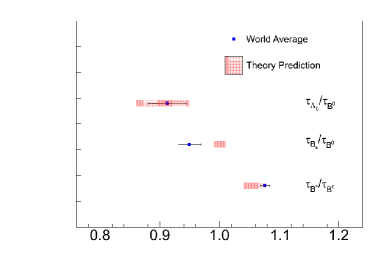
Figure 1: Current lifetime ratios for different $B$ hadrons with theoretical predictions from Ref. ref:timeratio .

II.1 $B^{0}_{s}$ lifetime measurements

The $B^{0}_{s}$ meson can decay directly or decay after it oscillates to $\bar{B}^{0}_{s}$. Time evolution of an arbitrary system $a(t)|B^{0}_{s}\rangle+b(t)|\bar{B}^{0}_{s}\rangle$ is governed by the Schr$\ddot{{\rm o}}$dinger Equation

$$i\frac{d}{dt}\left(\begin{array}[]{c}a\\ b\end{array}\right)=\left(M-i\frac{\Gamma}{2}\right)\left(\begin{array}[]{c}a\\ b\end{array}\right),$$ (2)

where $M$ and $\Gamma$ are mass and decay matrices. Two mass eigenstates $B^{0}_{L}$ and $B^{0}_{H}$ appear as a result of this mixing property. The eigenstates have different decay widths $\Gamma_{L}$ and $\Gamma_{H}$. The average decay width is defined as $\Gamma=(\Gamma_{L}+\Gamma_{H})/2$, while the decay width difference is $\Delta\Gamma=\Gamma_{L}-\Gamma_{H}$. $\Delta\Gamma$ also probes new physics since it’s related to quantity $\phi_{s}$ by $\Delta\Gamma=2|\Gamma_{12}|\cos(\phi_{s})$, where $\phi_{s}={\rm arg}(-M_{12}/\Gamma_{12})$, while $\Gamma_{12}$ and $M_{12}$ are matrix elements coming from the box diagram as shown in Fig. 2. New physics is likely to increase $\phi_{s}$, so $\Delta\Gamma$ could be smaller than the Standard Model prediction.

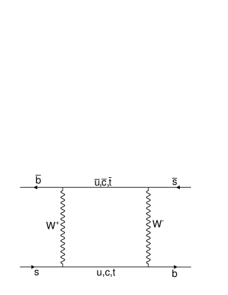
Figure 2: Feynman diagram for $B^{0}_{s}-\bar{B}^{0}_{s}$ mixing.

II.1.1 Results from $B^{0}_{s}\rightarrow J/\psi\phi$ channel

The data at CDF (1.7 fb^-1) and at D0 (2.8 fb^-1) were collected by di-muon triggers ref:CDFd ; ref:D0d which preferentially selects events containing $J/\psi\rightarrow\mu^{+}\mu^{-}$ decays. An artificial neural network is trained to separate signal and combinatorial backgrounds at CDF, which yields about 2500 signal events, while a cut based selection procedure is used to select data at D0, giving about 2000 signal events. The mass projections from CDF and D0 are shown in Fig. 3 and Fig. 4.

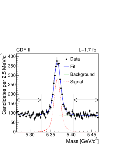
Figure 3: The invariant mass distribution of $B^{0}_{s}$ candidates from CDF

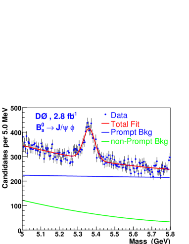
Figure 4: The invariant mass distribution of $B^{0}_{s}$ candidates from D0

Since $B^{0}_{s}$ is a pseudo-scalar meson, $J/\psi$ and $\phi$ are both vector mesons, the final states are admixtures of $CP$ eigenstates, where $S$ and $D$ waves are $CP$ even, $P$ wave is $CP$ odd. To separate the $CP$ eigenstates, the angular distribution are used ref:AS . $CP$ violation is predicted to be tiny in the Standard Model, so the $CP$ phase is fixed to zero at CDF, while it’s allowed to float at D0 with flavor tagging. To extract lifetime $\tau_{s}$ and decay width difference $\Delta\Gamma$, the final fit is done with an un-binned maximum likelihood method on mass, lifetime and angular variables.

The measured lifetime and decay width difference results from CDF are ref:CDFbs

$$\tau=1.52\pm 0.04({\rm stat})\pm 0.02({\rm syst})~{}{\rm ps}$$

$$\Delta\Gamma=0.08\pm 0.06({\rm stat})\pm 0.01({\rm syst})~{}{\rm ps^{-1}}$$

where $CP$ conservation is assumed, and the lifetime fit projection is shown in Fig. 5. At D0, the $CP$ violation phase is allowed to float (with external constraint on strong phases from $B^{0}\rightarrow J/\psi K^{*0}$), the results are ref:D0bs

$$\tau=1.52\pm 0.05({\rm stat})\pm 0.01({\rm syst})~{}{\rm ps}$$

$$\Delta\Gamma=0.19\pm 0.07({\rm stat})^{+0.02}_{-0.01}({\rm syst})~{}{\rm ps^{-1}}$$

The lifetime fit projection is shown in Fig. 6.

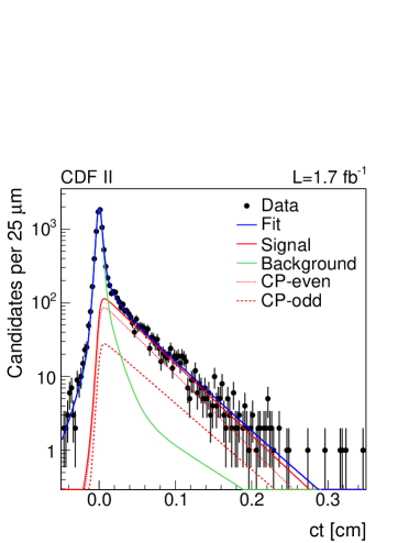
Figure 5: Proper decay time projection of the $B^{0}_{s}\rightarrow J/\psi\phi$ fit at CDF. $CP$ even fraction is dominant, and the slope difference of even and odd curves indicates decay width difference.

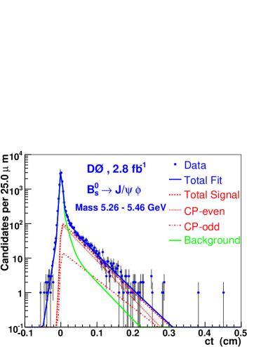
Figure 6: Proper decay time projection of the $B^{0}_{s}\rightarrow J/\psi\phi$ fit at D0.

The systematic errors are controlled very well at both CDF and D0. Systematic errors considered at CDF include background angular distribution, mass model, lifetime resolution model, $B^{0}\rightarrow J/\psi K^{*0}$ contamination, detector acceptance, and silicon detector alignment. Systematic errors considered at D0 include procedure test, acceptance, reconstruction algorithm, background model, and detector alignment.

II.1.2 Results from $B^{0}_{s}\rightarrow D_{s}(\phi\pi)\pi X$ channel

This channel is different from $B^{0}_{s}\rightarrow J/\psi\phi$, because it’s flavor specific, i.e. $B^{0}_{s}$ can only decay into $D^{-}_{s}\pi^{+}X$, while $\bar{B}^{0}_{s}$ can only decay into $D^{+}_{s}\pi^{-}X$. By fitting the signal with one exponential function, the obtained lifetime is related to average decay width and decay width difference by

$$\tau(B^{0}_{s})_{fs}=\frac{1}{\Gamma}(1+(\frac{\Delta\Gamma}{2\Gamma})^{2})/(1-(\frac{\Delta\Gamma}{2\Gamma})^{2})$$ (3)

assuming no $CP$ violation. So it can be used to constrain $\Gamma$ and $\Delta\Gamma$ in the global fit.

The result is obtained at CDF only, from both fully reconstructed $B^{0}_{s}\rightarrow D_{s}\pi$ and partially reconstructed channels such as $B^{0}_{s}\rightarrow D_{s}\rho(\pi^{+}\pi^{0})$ where the $\pi^{0}$ is not reconstructed. In the partially reconstructed channels, a “K” factor is introduced to correct the proper decay time for missing mass and transverse momentum

$$ct=\frac{L_{xy}m^{rec}_{B}}{p_{T}}K$$

where $L_{xy}$ is the projection of decay length in the $x-y$ plane, $m^{rec}_{B}$ is reconstructed mass, $p_{T}$ is reconstructed transverse momentum, and

$$K=\frac{m_{B}p_{T}}{m^{rec}_{B}p^{true}_{T}}$$

where $m_{B}$ is the true mass and $p^{true}_{T}$ is the true transverse momentum. The “K” factor distributions for different partially reconstructed channels are obtained from Monte Carlo and shown in Fig. 7.

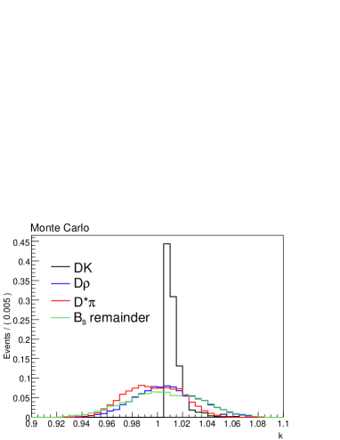
Figure 7: K factor distribution for each channel. The $DK$ channel is fully reconstructed, but treated in the same way, since the $K$ track is misidentified and a $K$ factor is needed.

The data (1.3 fb^-1) were collected by displaced-vertex trigger ref:svt at CDF. The trigger takes the advantage of the long lifetime of $B$ mesons and selects events within some impact parameter range ($120~{}\mu m\leq d_{0}\leq 1000~{}\mu m$) with respect to the primary vertex. The trigger makes it possible to select $B$ signal in large QCD backgrounds at CDF but also removes signal events which decay early. The lifetime bias is corrected using a trigger efficiency curve obtained from Monte Carlo.

The lifetime is extracted from a two-step fit. First a mass-only fit is done to extract relative fractions of various modes and backgrounds. The corresponding mass shapes are obtained from either Monte Carlo or data. A lifetime-only fit is performed with fractions fixed from the previous mass-only fit, where the lifetime is the only free parameter and the final result is ref:bsfltime

$$\tau=1.518\pm 0.041({\rm stat})\pm 0.025({\rm syst})~{}{\rm ps}$$

The lifetime results for control samples, such as $B^{0}\rightarrow D^{-}(K^{+}\pi^{-}\pi^{-})\pi^{+}$, $B^{0}\rightarrow D^{*-}(\bar{D}^{0}(K^{+}\pi^{-})\pi^{-})\pi^{+}$, and $B^{+}\rightarrow\bar{D}^{0}(K^{+}\pi^{-})\pi^{+}$, all agree well with PDG values.

Fig. 8 compares this result with all published results from flavor specific channels. The previous PDG value is dominated by the D0 result in 2006 from $B^{0}_{s}$ semileptonic channels. This new result agrees with the PDG 2007 value, but the central value is higher.

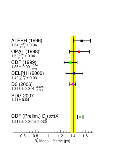
Figure 8: $B^{0}_{s}$ lifetime results from flavor specific channels.

II.2 $B_{c}$ lifetime measurement

The doubly heavy $B_{c}$ meson is an interesting QCD laboratory, where both $b$ and $c$ quarks can decay as well as annihilate. The lifetime is expected to be much shorter than light $B$ mesons. Current theory predictions span from 0.47 ps to 0.59 ps ref:bctheory , so experimental result with small uncertainty will be useful to constrain the theories.

Both CDF and D0 have measured the $B_{c}$ lifetime from $B_{c}\rightarrow J/\psi lX$ semileptonic channels, and data are collected by the di-muon trigger. At CDF both $B_{c}\rightarrow J/\psi\mu X$ and $B_{c}\rightarrow J/\psi eX$ decays are reconstructed from 1.0 fb^-1 data. At D0 only $B_{c}\rightarrow J/\psi\mu X$ is reconstructed from 1.3 fb^-1 data. Because of the missing momentum of the neutrino, a “K” factor is also needed from Monte Carlo to correct the reconstructed lifetime value. Here the mass is taken from the measured value ref:bcmass instead of the reconstructed value, so the “K” factor takes the form

$$K=\frac{p_{T}(J/\psi l)}{p_{T}(B_{c})}$$

The main challenge of the analysis is the various and dominant backgrounds which include: 1) fake $J/\psi$ plus true lepton, 2) true $J/\psi$ plus fake lepton, 3) true $J/\psi$ and lepton from different $b$ quarks, 4) prompt $J/\psi$ background, 5) residual conversion (for electron channel only). At CDF, the shape of the proper decay time distributions of all backgrounds are modeled and calibrated carefully from either data or Monte Carlo, and the lifetime is extracted from a lifetime-only fit. At D0, the mass shape of signal and backgrounds are also modeled, and the lifetime is extracted from a mass-lifetime simultaneous fit.

The measured lifetime results at CDF from both muon and electron channels are ref:CDFbc

$$c\tau=179.1^{+32.6}_{-27.2}({\rm stat})~{}\mu m\ ({\rm muon\ channel})$$

$$c\tau=121.7^{+18.0}_{-16.3}({\rm stat})~{}\mu m\ ({\rm electron\ channel})$$

and the combined result from two channels is given by

$$\tau(B_{c})=0.475^{+0.053}_{-0.049}({\rm stat})\pm 0.018({\rm syst})~{}{\rm ps}$$

The same lifetime measured at D0 is ref:D0bc

$$\tau(B_{c})=0.448^{+0.038}_{-0.036}({\rm stat})\pm 0.032({\rm syst})~{}{\rm ps}$$

The measured $B_{c}$ lifetime values from CDF and D0 agree with each other well, and since the Tevatron is currently the only place which can produce $B_{c}$ mesons, one can make a weighted world average with all the previous measurements from the Tevatron. The plot is shown in Fig. 9, and the weighted average is

$$\tau(B_{c})=0.459\pm 0.037~{}{\rm ps}\$$

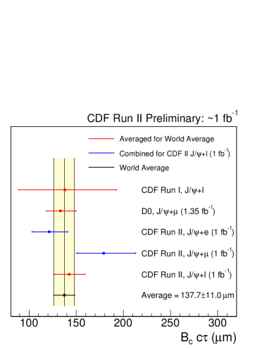
Figure 9: Comparison of $B_{c}$ lifetime with CDF and D0 RunI results, and an weighted average (assuming no correlations among) those measurements.

III $B^{0}_{s}$ Mixing

As shown in Fig. 2, $B^{0}_{s}$ oscillates through a box diagram. The oscillation frequency $\Delta m_{s}$ is the mass difference of heavy and light eigenstates $\Delta m_{s}\equiv m_{H}-m_{L}$, which are related to the off diagonal element $M_{12}$ of the mass matrix by

$$\Delta m_{s}=2|M_{12}|$$ (4)

With the oscillation frequency from the $B^{0}$ system, one can take the ratio to cancel most of the theoretical uncertainties and get

$$\frac{\Delta m_{s}}{\Delta m_{d}}\propto\frac{|V_{ts}|^{2}}{|V_{td}|^{2}}$$ (5)

which is very important for constraining the CKM unitary triangle with measurements of other CKM matrix elements and some theory inputs.

The probability for a $B^{0}_{s}$ meson to mix or not as a function of time is proportional to

$$P(t)_{B^{0}_{s}\rightarrow B^{0}_{s},\bar{B}^{0}_{s}}\propto 1\pm\cos{\Delta m_{s}t}$$ (6)

And one needs to identify the flavor of the meson at both production and decay time to see if it’s mixed or unmixed. By reconstructing flavor specific channels, the flavor at decay time can be identical to the charge of the daughter particle. To identify the flavor at production time, two algorithms are generally used at the Tevatron. On the same side of the reconstructed $B^{0}_{s}$ meson, one looks at the charge of the kaon from fragmentation processes. On the opposite side, one can look at the charge of leptons from semileptonic decays or the jet charge of the other $b$ quark. However, many things can dilute the tagging power, for example, the kaon mis-identification and low efficiency on the same side, mixing of neutral $B$ mesons and sequential $b$ decays on the opposite side. Thus, a dilution factor ${\cal D}$ is introduced, and it modifies Eq. 6.

$$P(t)_{B^{0}_{s}\rightarrow B^{0}_{s},\bar{B}^{0}_{s}}\propto 1\pm{\cal D}\cos{\Delta m_{s}t}$$ (7)

and $(1+{\cal D})/2$ gives correct tagging probability.

Following the CDF measurement in 2006 with $\Delta m_{s}=17.77\pm 0.10({\rm stat})\pm 0.07({\rm syst})~{}{\rm ps}$, D0 now has a new measurement with 2.4 fb^-1 data. The first 1.3 fb^-1 belongs to Run IIa period and the other 1.1 fb^-1 belongs to Run IIb when an additional silicon layer was installed at D0. Both hadronic and semileptonic decays are collected by inclusive single or di-muon triggers at D0. Most of the reconstructed channels and signal yields are listed in Tab. 1, in addition, 1.2 fb^-1 of $B^{0}_{s}\rightarrow\mu^{+}D^{-}_{s}(K^{0}_{s}K^{-})$ decays from Run IIa give about 600 signal events.

Table 1: Reconstructed channels and yields in $B^{0}_{s}$ mixing measurement

Channel	Run IIa	Run IIb	Total
$\mu^{+}D^{-}_{s}(\phi\pi^{-})$	$28238\pm 339$	$16539\pm 239$	$44777\pm 415$
$e^{+}D^{-}_{s}(\phi\pi^{-})$	$1142\pm 83$	$548\pm 45$	$1663\pm 102$
$\pi^{+}D^{-}_{s}(\phi\pi^{-})$	$159\pm 13$	$90\pm 11$	$249\pm 17$
$\mu^{+}D^{-}_{s}(K^{*0}K^{-})$	$11649\pm 661$	$6449\pm 616$	$18098\pm 903$

An amplitude $A$ is introduced as shown in

$$P(t)_{B^{0}_{s}\rightarrow B^{0}_{s},\bar{B}^{0}_{s}}\propto 1\pm A{\cal D}\cos{\Delta m_{s}t}$$ (8)

where $A$ can be fitted by fixing $\Delta m_{s}$ at different points, the true $\Delta m_{s}$ value is indicated when the fitted A is consistent with unity, otherwise a sensitivity at 95% C.L. can be defined by the probe $\Delta m_{s}$ value at which

$$1.645\sigma_{A}(\Delta m_{sens})=1.0$$ (9)

Individual amplitude scans vs. probe $\Delta m_{s}$ were done separately for different channels and combined using COMBOS program ref:combine . The combined amplitude scan is shown in Fig. 10. The likelihood profile is obtained from the combined amplitude scan using the formula ref:likelihood

$$\Delta Ln{\cal L}=-Ln{\cal L}(\Delta m_{s})+Ln{\cal L}(\infty)=\frac{\frac{1}{2}-A_{fit}(\Delta m_{s})}{\sigma^{2}_{A}}$$ (10)

and the profile is shown in Fig. 11. The measured $\Delta m_{s}$ and its errors are derived by fitting a quadratic function to it, giving ref:bsmixing

$$\Delta m_{s}=18.53\pm 0.93({\rm stat})\pm 0.30({\rm syst})$$ (11)

which has a total significance of 2.9 $\sigma$.

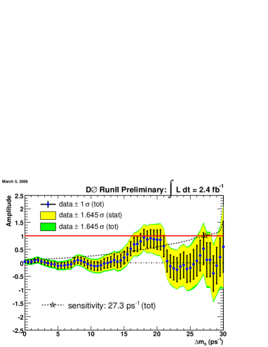
Figure 10: $B^{0}_{s}$ mixing combined amplitude scan.

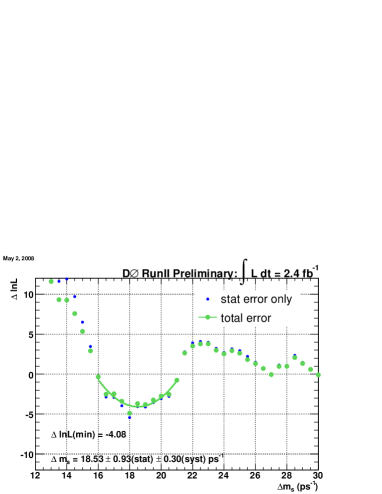
Figure 11: $B^{0}_{s}$ combined likelihood profile, which is done with statistical error and total error on amplitude $A$ separately. An estimate of the $\Delta m_{s}$ systematic error is obtained by subtracting, in quadrature, the error derived from statistical-error-only likelihood curve from that of the total-error curve.

IV $D^{0}$ Mixing

Since the discovery of charm quark in 1974, physicists have been trying to observe oscillations of the neutral charm meson. Unlike the kaon or $B$ systems, the oscillation frequency in the charm system is predicted to be very small. In the Standard Model, $D^{0}$ mixing occurs through two processes. The “long range” mixing can be estimated using strong interaction models. The “short range” process is negligible in the standard model, however, exotic weakly interacting particle from new physics could enhance the short-range process.

Recent $D^{0}$ mixing evidence has been found at the $B$ factories in 2007. The $Belle$ Collaboration found direct evidence by comparing the decay time distributions for $D^{0}$ decays to the $CP$-eigenstates $K^{+}K^{-}$ and $\pi^{+}\pi^{-}$ with that for the $CP$-mixed state $K^{-}\pi^{+}$. The evidence found in the $BABAR$ experiment is the decay rate difference of doubly-Cabibbo-suppressed (DCS) $D^{0}\rightarrow K^{+}\pi^{-}$ decay and Cabibbo favored (CF) $D^{0}\rightarrow K^{-}\pi^{+}$ decay. The ratio of decay rates can be approximated as a simple quadratic function of proper decay time and mean $D^{0}$ lifetime, with the assumption of $CP$ conservation and a small value of $x=\Delta m/\Gamma$ and $y=\Delta\Gamma/2\Gamma$,

$$R(t/\tau)=R_{D}+\sqrt{R_{D}}y^{\prime}(t/\tau)+\frac{x^{\prime 2}+y^{\prime 2}}{4}(t/\tau)^{4}$$ (12)

where $R_{D}$ is the square of the ratio of DCS to CF amplitudes, $x^{\prime}$ and $y^{\prime}$ are linear combinations of $x$ and $y$ as

$$x^{\prime}=x\cos\delta+y\sin\delta$$

$$y^{\prime}=-x\sin\delta+y\cos\delta$$

where $\delta$ is the strong phase difference between the DCS and CF amplitudes. In the absence of mixing, $x^{\prime}$ and $y^{\prime}$ are both zero.

At CDF, the same kind of evidence is found as in $BABAR$, but probed over a much wider $D^{0}$ decay time range. Events are selected with the displaced-vertex trigger using about 1.5 fb^-1 data. The “right-sign” (RS) CF decay chain $D^{*+}\rightarrow\pi^{+}D^{0}$, $D^{0}\rightarrow K^{-}\pi^{+}$, and the “wrong sign” (WS) decay chain $D^{*+}\rightarrow\pi^{+}D^{0}$, $D^{0}\rightarrow K^{+}\pi^{-}$ are reconstructed. The relative charges of the two pions gives the “sign” of the decay chain and extra cuts are applied to reduce background to the WS signal from RS decays. The data are divided into 20 bins of $t/\tau$ ranging from 0.75 to 10.0 with bin size increasing from 0.25 to 2.0 to reduce statistical uncertainty at larger times. The ratio $R$ is determined at each bin and a least-squares parabolic fit of the data is done with Eq. 12. The fit is shown in Fig. 12, and final results are shown in Table. 2 ref:d0mixing .

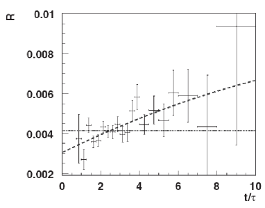
Figure 12: Ratio of prompt $D^{*}$ “wrong sign” to “right sign”decays as a function of normalized proper decay time. The dashed curve is from a least-squares parabolic fit, the dotted line is the fit assuming no mixing

Table 2: Fit results for the $R(t/\tau)$ distribution

Fit type	$R_{D}(10^{-3})$	$y^{\prime}(10^{-3})$	$x^{\prime 2}(10^{-3})$	$\chi^{2}/d.o.f$
Unconstrained	$3.04\pm 0.55$	$8.5\pm 7.6$	$-0.12\pm 0.35$	19.2/17
Physically allowed	$3.22\pm 0.23$	$6.0\pm 1.4$	$0$	19.3/18
No mixing	$4.15\pm 0.10$	$0$	$0$	36.8/19

To determine the consistency of the data with the no-mixing hypothesis, Bayesian contours are computed with likelihood and a flat prior. The contours are insensitive to modest changes in the prior, and shown in Fig. 13. The no-mixing point lies on the contour which excludes the region containing a probability of $1.5\times 10^{-4}$, equivalent to 3.8 Gaussian standard deviations. Alternative procedures are also used to determine the probability for no mixing, and all give consistent results.

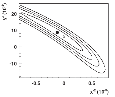
Figure 13: Bayesian probability contours in the $x^{\prime 2}-y^{\prime}$ parameter space corresponding to one through four equivalent Gaussian standard deviations. The closed circle shows the unconstrained fit, the open diamond shows physically allowed fit ($x^{\prime 2}\geq 0$), the cross shows the no-mixing point.

V Summary

The most precise $B^{0}_{s}$ lifetime and decay width difference have been measured directly from the $B^{0}_{s}\rightarrow J/\psi\phi$ channel from both CDF and D0 experiments. The measured lifetime is also consistent with the value from $B^{0}_{s}$ flavor specific channel. Together, the recent results confirm the theory prediction that $\tau_{s}/\tau_{d}\sim 1$. The lifetime measurement result for the heavy $B_{c}$ meson can provide good experimental input for the theory calculation which still has a huge uncertainty. The fast oscillation of $B^{0}_{s}$ mesons has been measured at CDF in 2006 and is now verified by the D0 experiment with results from combined channels. While $D^{0}$ mixing is predicted to be quite small in the Standard Model, the evidence has been found at CDF followed the first observation at $B$ factories last year.