Recursive Schrödinger Equation Approach to Faster Converging Path Integrals

Abstract

By recursively solving the underlying Schrödinger equation, we set up an efficient systematic approach for deriving analytic expressions for discretized effective actions. With this we obtain discrete short-time propagators for both one and many particles in arbitrary dimension to orders which have not been accessible before. They can be used to substantially speed up numerical Monte Carlo calculations of path integrals, as well as for setting up a new analytical approximation scheme for energy spectra, density of states, and other statistical properties of quantum systems.

I Introduction

The central object in the path-integral formulation of quantum statistics is the (Euclidean) transition amplitude $A(a,b;t)=\langle b|e^{-t\hat{H}}|a\rangle$ feynman ; feynmanhibbs ; feynmanstat ; kleinertbook . The starting point in setting up this formalism is the completeness relation

$$A(a,b;t) = \int dq_{1}\cdots\int dq_{N-1}$$ (1)

$$\times\,A(a,q_{1};\varepsilon)\cdots A(q_{N-1},b;\varepsilon)\,,$$

where $\varepsilon=t/N$ denotes the time-slice width. To leading order in $\varepsilon$ the short-time transition amplitude reads in natural units

$$A(q_{n},q_{n+1};\varepsilon)=$$ (2)

$$=\frac{1}{(2\pi\varepsilon)^{d/2}}\exp\left[-\frac{(q_{n+1}-q_{n})^{2}}{2\varepsilon}-\varepsilon V(x_{n})\right]\,,$$

where the potential $V$ is evaluated at the mid-point coordinate $x_{n}=(q_{n}+q_{n+1})/2$. Substituting (2) in the completeness relation (1), the deviation of the obtained discrete amplitude from the continuum result turns out to be of the order $O(\varepsilon)$. This slow convergence to the continuum is the major reason for the low efficiency of the ubiquitous Path Integral Monte Carlo simulations ceperley , especially in numeric studies of Bose-Einstein condensation phenomena pilati2006 ; zhang ; pilati2008 , quantum phase transitions and phase diagrams at low temperatures vitali ; kim . Thus, in order to accelerate numerical calculations for statistical properties of quantum systems, it is indispensable to develop more efficient algorithms. The existence of such algorithms has been established recently predescu .

To this end we worked out and numerically verified in a series of recent papers prl-speedup ; prb-speedup ; pla-euler ; pre-ideal an efficient analytical procedure for improving the convergence of path integrals for single-particle transition amplitudes to the order $O(\varepsilon^{p})$ for arbitrary values of $p$. This was achieved by studying how discretizations of different coarseness are related to a hierarchy of effective discrete-time actions which improve the convergence in a systematic way. In Ref. pla-manybody we presented an equivalent approach which is based on a direct path-integral calculation of intermediate time amplitudes to the order $O(\varepsilon^{p})$. The inherent simplicity of these direct calculations made it possible to extend the procedure to general many-body theories in arbitrary dimension and to obtain explicit results for the effective actions up to level $p=5$. It turned out that increasing $p$ leads to an exponential rise in complexity of the effective actions which, ultimately, limits the maximal value of $p$ one can practically work with. These limitations of existing approaches, in particular in the case of many-body theories, are still below the calculational barrier stemming from this rise in complexity. This is a strong indication that new and more efficient calculational schemes must exist which should considerably improve the convergence of path integrals for general many-body theories. The availability of analytic expressions for higher $p$ effective actions is essential for numerical calculations of path integrals with high precision. Obtaining the information on energy spectra is just one important example of calculations that require high-precision numerical results. Furthermore, since the structure of higher order terms of effective actions is governed by the quantum dynamics of the system, it can be used for extracting analytical information about the system properties.

As is well known, in concrete calculations it is always easier to solve the underlying Schrödinger equation than to directly evaluate the corresponding path integral. For instance, in the case of particular potentials the Schrödinger equation approach allows an efficient recursive scheme to calculate perturbation series up to very high orders S1 ; S2 ; S3 ; S4 ; S5 . With this in mind, we develop in the present paper a new and more efficient recursive approach for deriving the short-time transition amplitude from the underlying Schrödinger equation. To this end we proceed as follows. Section 2 presents the instructive case of a single one-dimensional particle moving in a general potential. The maximal level obtained by the new method is $p=35$, and thus compares favorably with the best result $p=9$ of previous approaches. In Section 3 we focus on the restricted problem of evaluating the velocity independent part of the discrete-time effective potential. We derive the differential equations for the velocity independent effective potential of a single one-dimensional particle and solve them for the case of a general potential up to level $p=37$. Section 4 extends the results of Section 2 to the case of a general many-body theory in $d$ dimensions. We derive the differential equations for the general many-body effective potential and solve them up to level $p=10$. Both the equations and their solution are presented in Section 5 in a diagrammatic form which is similar to the recursive graphical construction of Feynman diagrams worked out in the series C1 ; C2 ; C3 ; C4 ; C5 ; C6 . With this we illustrate the inherent combinatoric nature of determining the discrete-time effective potential. The growing number of diagrams with level $p$ leads to an increasing complexity of the expression for the discrete-time effective potential. We end by commenting on how this growth in complexity limits maximal attainable values of $p$. Throughout the paper we describe some important envisaged applications of the derived discretized effective actions for calculating statistical properties of relevant quantum systems. These applications include not only numerical calculations but also a new analytical approximation scheme which was made possible through the availability of high level effective actions.

II One particle in One Dimension

We start with calculating the transition amplitude $A(q,q^{\prime};\varepsilon)$ for one particle in one dimension. It obeys the symmetry

$$A(q,q^{\prime};\varepsilon)=A(q^{\prime},q;\varepsilon)$$ (3)

and satisfies the time-dependent Schrödinger equations

$$\left[\frac{\partial}{\partial\varepsilon}-\frac{1}{2}\,\frac{\partial^{2}}{\partial q^{2}}+V(q)\right]A(q,q^{\prime};\varepsilon) = 0\,,$$ (4)

$$\left[\frac{\partial}{\partial\varepsilon}-\frac{1}{2}\,\frac{\partial^{2}}{\partial q^{\prime 2}}+V(q^{\prime})\right]A(q,q^{\prime};\varepsilon) = 0$$ (5)

with the initial condition

$$A(q,q^{\prime};0)=\delta(q-q^{\prime})\,.$$ (6)

In terms of the deviation $\bar{x}=(q^{\prime}-q)/2$ and the mid-point coordinate $x=(q+q^{\prime})/2$, both equations are rewritten according to

$$\left[\frac{\partial}{\partial\varepsilon}-\frac{1}{8}\,\partial^{2}-\frac{1}{8}\,\bar{\partial}^{2}+\frac{1}{2}\,(V_{+}+V_{-})\right]A = 0\,,$$ (7)

$$\left[-\,\partial\bar{\partial}+2\,(V_{+}-V_{-})\right]A = 0\,,$$ (8)

where we have introduced $V_{\pm}=V(x\pm\bar{x})$ as an abbreviation. Their solution may be written in the form

$$A=\frac{1}{\sqrt{2\pi\varepsilon}}\exp\left[-\frac{2}{\varepsilon}\,\bar{x}^{2}-\varepsilon W(x,\bar{x};\varepsilon)\right]\,,$$ (9)

where the effective potential $W(x,\bar{x};\varepsilon)$ is an even function of $\bar{x}$ due to the symmetry (3) of the Euclidean transition amplitude. Note that Eq. (2) represents an approximation to the exact form (9) up to order $O(\varepsilon)$. Substituting (9) in (7) and (8) yields

$$W+\bar{x}\,\frac{\partial W}{\partial\bar{x}}+\varepsilon\,\frac{\partial W}{\partial\varepsilon}-\frac{1}{8}\,\varepsilon\,\partial^{2}W-\frac{1}{8}\,\varepsilon\,\bar{\partial}^{2}W$$

$$\quad\ +\,\frac{1}{8}\,\varepsilon^{2}\,(\partial W)^{2}+\frac{1}{8}\,\varepsilon^{2}\,(\bar{\partial}W)^{2}=\frac{1}{2}\,(V_{+}+V_{-})\,,$$ (10)

$$\bar{x}\,\partial W-\frac{1}{4}\,\varepsilon\,\partial\bar{\partial}W+\frac{1}{4}\,\varepsilon^{2}\,\partial W\bar{\partial}W=\frac{1}{2}\,(V_{+}-V_{-})\,.$$ (11)

Both partial differential equations determine the effective potential $W(x,\bar{x};\varepsilon)$ and thus the transition amplitude $A(q,q^{\prime};\varepsilon)$. The initial condition (6) implies that $W$ is regular in the vicinity of $\varepsilon=0$, i.e. it may be expanded in a power series in $\varepsilon$. We are interested in using $W$ to systematically speed up the convergence of discrete amplitudes with $N$ time slices to the continuum limit. This is done by evaluating $W$ to higher powers in $\varepsilon$. According to Eq. (2) the dominant term for the short-time propagation is the diffusion relation $\bar{x}^{2}\propto\varepsilon$. Therefore, we expand $W$ in a double power series in both $\varepsilon$ and $\bar{x}^{2}$:

$$W(x,\bar{x};\varepsilon)=\sum_{m=0}^{\infty}\sum_{k=0}^{m}c_{m,k}(x)\,\varepsilon^{m-k}\bar{x}^{2k}\ .$$ (12)

Restricting the sum over $m$ from 0 to $p-1$ leads to a discrete amplitude that converges to the continuum result as $\varepsilon^{p}$, i.e. as $1/N^{p}$. For later convenience we define all coefficients $c_{m,k}$, which are not explicitly used in Eq. (12), to be zero, i.e. we set $c_{m,k}=0$ whenever the condition $m\geq k\geq 0$ is not satisfied.

Substituting the expansion (12) into the partial differential equations (II) and (11) leads to two equivalent recursion relations. The second recursion relation turns out to be more difficult to solve to higher orders as it directly determines not the coefficients $c_{m,k}(x)$ but their first derivatives. For this reason we restrict ourselves in the remainder of this section to the recursion relation following from Eq. (II). The diagonal coefficients are given by

$$c_{m,m}=\frac{V^{(2m)}}{(2m+1)!}\,,$$ (13)

while off-diagonal coefficients satisfy the recursion relation

$$8(m+k+1)\,c_{m,k}=(2k+2)(2k+1)\,c_{m,k+1}$$

$$\,\,+c_{m-1,k}^{\prime\prime}-\sum_{l=0}^{m-2}\,\sum_{r}c_{l,r}^{\prime}\,c_{m-l-2,k-r}^{\prime}$$

$$\,\,-\sum_{l=1}^{m-2}\,\sum_{r}2\,r(2k-2r+2)\,c_{l,r}\,c_{m-l-1,k-r+1}\,,$$ (14)

where the sum over $r$ goes from ${\rm max}\{0,k-m+l+2\}$ to ${\rm min}\{k,l\}$ in accordance with the restriction that $c_{m,k}=0$ whenever the condition $m\geq k\geq 0$ is not satisfied. For a given value of $m$, the coefficients $c_{m,k}$ for $k=0,1,\ldots,m$ are determined as follows. The diagonal coefficient $c_{m,m}$ is directly given by (13), whereas the off-diagonal coefficients $c_{m,k}$ follow recursively from evaluating (14) for $k=m-1,\ldots,1,0$. This recursive solution method is schematically depicted in Fig. 1. Let us illustrate this procedure for the lowest levels. For $p=1$ we immediately obtain from (13)

$$c_{0,0}=V\,.$$ (15)

For $p=2$ we have to first determine $c_{1,1}$ from (13), yielding

$$c_{1,1}=\frac{V^{\prime\prime}}{6}\,.$$ (16)

Then recursion relation (14) states that $c_{1,0}$ follows from the previously determined coefficients according to

$$c_{1,0}=\frac{1}{16}c^{\prime\prime}_{0,0}+\frac{1}{8}c_{1,1}\,.$$ (17)

From (15)–(17) we then read off the result

$$c_{1,0}=\frac{V^{\prime\prime}}{12}\,.$$ (18)

Similarly, we find for $p=3$

$$c_{2,2}=\frac{V^{(4)}}{120}\,,$$ (19)

$$c_{2,1}=\frac{1}{32}\,c^{\prime\prime}_{1,1}+\frac{3}{8}\,c_{2,2}=\frac{V^{(4)}}{120}\,,$$ (20)

$$c_{2,0}=\frac{1}{24}\,c^{\prime\prime}_{1,0}+\frac{1}{12}\,c_{2,1}-\frac{1}{24}\,(c^{\prime}_{0,0})^{2}=\frac{V^{(4)}}{240}-\frac{V^{\prime 2}}{24}\,.$$ (21)

The outlined procedure continues in the same way for higher levels $p$. We have automatized this procedure and implemented it using the Mathematica 6.0 package mathematica for symbolic calculus. Using this we determined the effective action for a one-dimensional particle in a general potential up to the level $p=35$. Although the effective actions grow in complexity with level $p$, the Schrödinger equation method for calculating the discrete-time effective actions turns out to be extremely efficient. The ultimate value of $p=35$ far surpasses the previously obtained best result of $p=9$, and is only limited by the sheer size of the expression for the effective action of a general theory at such a high level.

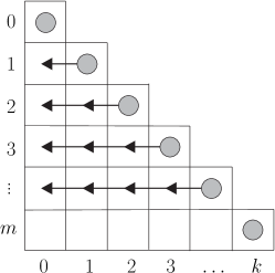
Figure 1: (Color online) Order in which the coefficients $c_{m,k}$ are calculated. Diagonal ones follow from Eq. (13), off-diagonal ones from the recursion relation (14).

The whole technique can be pushed much further when working on specific potential classes. For example, for a particle moving in a quartic potential we have obtained effective actions up to $p=140$. Similar levels have been achieved for higher-order polynomial potentials. The increase in level and the decrease in size of the expressions for the effective actions originate from functional relations between the potential and its derivatives. These relations are particularly simple in the case of polynomial interactions where all the derivatives of the potential above a certain degree vanish. However, the benefits of working within a specific class of potentials are not only limited to polynomial interactions. For example, the functional relations for the modified Pöschl-Teller potential have allowed us to obtain effective actions up to level $p=40$ speedup .

As already stated, the principal rationale behind constructing high-level effective actions is to use them for speeding up Monte Carlo calculations. However, having obtained explicit expressions for effective actions to such high levels, it now becomes possible to use them extensively in both numerical and analytical calculations. In particular, having obtained an extremely precise knowledge of the short-time propagation of a system, it is possible to use standard resummation techniques such as the Padé and the Borel method to extract useful information about its behavior for long propagation times.

The derived effective actions can also be applied to systematically improve the Numerical Matrix Diagonalization (NMD) method pollockceperley ; sethia1990 ; sethia1999 for calculating energy eigenvalues and eigenstates. Note that the propagation time $t$ used in the NMD method is just a parameter which is chosen in such a way that it minimizes the error associated with the calculated energy eigenvalues. Therefore, it is always possible to select this parameter to be small, so that the obtained expansion of the ideal effective action can be used to substantially improve NMD calculations. Furthermore, in this case we can even use analytic $N=1$ approximation for the path integral. In this approximation there are no integrals to perform in Eq. (1) and the amplitude is directly given by the analytic expression (9). Using such extremely rough discretizations is only possible if one has determined the ideal effective action to very high orders $p$. In effect, one compensates without loss of precision the increase of discretization coarseness with the input of new analytical information concerning the propagation time which is contained in the effective action. In this way, without any integration or resummation techniques, we can calculate large number of highly accurate energy eigenvalues, avoiding the usually needed limit $t\to\infty$ which is difficult to approach. The large number of precise energy eigenvalues obtained by using this improved NMD method allows for calculating amplitudes for longer propagation times using the spectral decomposition. This also makes it possible to calculate partition functions as well as global, local, and bilocal densities of states or other relevant statistical quantities with high accuracy.

III Velocity Independent Part of Effective Potential

The velocity independent part of the effective potential $W_{0}(x;\varepsilon)\equiv W(x,0;\varepsilon)$ determines diagonal transition amplitudes. Although it does not contain all the information which is needed for constructing the effective action, it is of interest for determining physical quantities such as the particle density and the energy spectra. This object is also much simpler than the full $W$. In addition, the relation between $V$ and $W_{0}$ allows us to visualize the effects of quantization and discretization for a given potential. In this section we derive the differential equation for $W_{0}$ for a single particle moving in one dimension.

Both Eqs. (7) and (8) contain derivatives with respect to $\bar{x}$, so it is impossible to set $\bar{x}=0$ and obtain equations for $W_{0}$. However, differentiating Eq. (8) with respect to $\bar{x}$ we get

$$\partial\bar{\partial}^{2}A=4\,\partial VA+\ldots\ ,$$ (22)

where the dots denote terms which vanish when $\bar{x}\to 0$. Thus, differentiating Eq. (7) with respect to $x$ and substituting the above result we obtain an equation which does not contain derivatives with respect to $\bar{x}$. Finally, setting $\bar{x}=0$ we find the differential equation for diagonal transition amplitudes

$$\left(\partial\frac{\partial}{\partial\varepsilon}-\frac{1}{8}\,\partial^{3}+\frac{1}{2}\,\partial V+V\partial\right)A(x,x;\varepsilon)=0\ .$$ (23)

Substituting $A(x,x;\varepsilon)=(2\pi\varepsilon)^{-1/2}\exp(-\varepsilon W_{0})$ then yields the equation for $W_{0}$:

$$\partial W_{0}+\frac{\varepsilon}{4}\left(8\,\partial\frac{\partial W_{0}}{\partial\varepsilon}-8W_{0}\,\partial W_{0}+8V\partial W_{0}-\partial^{3}W_{0}\right)$$ (24)

$$-\frac{\varepsilon^{2}}{4}\left(8\,\partial W_{0}\frac{\partial W_{0}}{\partial\varepsilon}-3\partial W_{0}\partial^{2}W_{0}\right)-\frac{\varepsilon^{3}}{4}\,(\partial W_{0})^{3}=\partial V\,.$$

This is solved in the form of the power series

$$W_{0}(x;\varepsilon)=\sum_{m=0}^{\infty}c_{m,0}(x)\varepsilon^{m}\,.$$ (25)

Inserting this into the differential equation (III) determines the coefficients $c_{m,0}$ through the simple recursion relation

$$(2m+1)\,c_{m,0}^{\prime}=\frac{1}{4}\,c_{m-1,0}^{\prime\prime\prime}-2\,Vc_{m-1,0}^{\prime}$$ (26)

$$+2\sum_{k=0}^{m-1}c_{k,0}^{\prime}\,c_{m-k-1,0}+2\sum_{k=1}^{m-1}k\,c_{k,0}\,c_{m-k-1,0}^{\prime}$$

$$-\frac{3}{4}\sum_{k=0}^{m-2}c_{k,0}^{\prime}\,c_{m-k-2,0}^{\prime\prime}+\frac{1}{4}\sum_{k=0}^{m-3}\,\sum_{l=0}^{m-k-3}c_{k,0}^{\prime}\,c_{l,0}^{\prime}\,c_{m-k-l-3,0}^{\prime}\,.$$

With this we have evaluated the velocity independent part of the effective potential up to level $p=37$ for a particle moving in a generic potential $V(x)$. As before, for specific potential classes one can go to much higher levels.

IV Many-Body Systems

Now we extend the calculations of Section 2 to the case of a general non-relativistic theory of $M$ particles in $d$ dimensions. The derivation of the equations for $W$ proceeds completely parallel to the case of one particle in one dimension. The Schrödinger equations now have the form

$$\left[\frac{\partial}{\partial\varepsilon}-\frac{1}{2}\,\sum_{i=1}^{M}\triangle_{i}+V(q)\right]A(q,q^{\prime};\varepsilon) = 0\,,$$ (27)

$$\left[\frac{\partial}{\partial\varepsilon}-\frac{1}{2}\,\sum_{i=1}^{M}\triangle^{\prime}_{i}+V(q^{\prime})\right]A(q,q^{\prime};\varepsilon) = 0\,,$$ (28)

where $\triangle_{i}$ and $\triangle^{\prime}_{i}$ stand for $d$-dimensional Laplacians over initial and final coordinates of particle $i$, while $q$ and $q^{\prime}$ are $d\times M$ dimensional vectors representing positions of all particles at the initial and final moment. Furthermore, the potential $V$ contains both the external potential and the respective interaction potentials between two and more particles. After substituting the $dM$-dimensional generalization of the expression for the transition amplitude (9) into the Schrödinger equations (27) and (28), we find the analogues of Eqs. (II) and (11) for the effective potential $W$

$$W+\bar{x}\cdot\bar{\partial}\,W+\varepsilon\frac{\partial W}{\partial\varepsilon}-\frac{1}{8}\,\varepsilon\partial^{2}W-\frac{1}{8}\,\varepsilon\bar{\partial}^{2}W$$

$$+\frac{1}{8}\,\varepsilon^{2}(\partial W)^{2}+\frac{1}{8}\,\varepsilon^{2}(\bar{\partial}W)^{2}=\frac{1}{2}\,(V_{+}+V_{-})\,,$$ (29)

$$\bar{x}\cdot\partial\,W-\frac{\varepsilon}{4}\,\partial\cdot\bar{\partial}\,W+\frac{\varepsilon^{2}}{4}(\partial W)\cdot(\bar{\partial}W)$$

$$=\frac{1}{2}\,(V_{+}-V_{-})\,.$$ (30)

Here we have used the definition $A\cdot B=A_{i}B_{i}$, where $i=1,2,\ldots,Md$ and repeated indices are summed over. Either of the above two equations for $W$ can be used to determine the appropriate short-time expansion as a double Taylor series in powers of $\varepsilon$ and even powers of $\bar{x}$:

$$W(x,\bar{x};\varepsilon)=\sum_{m=0}^{\infty}\,\sum_{k=0}^{m}\varepsilon^{m-k}\,W_{m,k}(x,\bar{x})\ ,$$ (31)

where $W_{m,k}(x,\bar{x})=\bar{x}_{i_{1}}\bar{x}_{i_{2}}\cdots\bar{x}_{i_{2k}}c_{m,k}^{i_{1},\ldots,i_{2k}}(x)$. It turns out to be advantageous to use recursion relations for the fully contracted quantities $W_{m,k}$ rather than the respective coefficients $c_{m,k}^{i_{1},\ldots,i_{2k}}$. In this way we avoid the computationally expensive symmetrization over all indices $i_{1},\ldots,i_{2k}$. Again it is easier to work with the first of the two equations for $W$. Substituting (31) into (29) directly yields the diagonal coefficients

$$W_{m,m}=\frac{1}{(2m+1)!}(\bar{x}\cdot\partial)^{2m}\,V\,.$$ (32)

The off-diagonal coefficients satisfy the recursion relation which represents a generalization of Eq. (14):

$$8\,(m+k+1)\,W_{m,k}=\partial^{2}W_{m-1,k}+\bar{\partial}^{2}W_{m,k+1}$$

$$-\sum_{l=0}^{m-2}\,\sum_{r}(\partial W_{l,r})\cdot(\partial W_{m-l-2,k-r})$$

$$-\sum_{l=1}^{m-2}\,\sum_{r}(\bar{\partial}W_{l,r})\cdot(\bar{\partial}W_{m-l-1,k-r+1})\,.$$ (33)

As before, the sum over $r$ goes from ${\rm max}\{0,k-m+l+2\}$ to ${\rm min}\{k,l\}$. The above recursion disentangles, in complete analogy with the previously outlined case of one particle in one dimension. To illustrate this we write down and solve the equations up to level $p=4$:

$$W_{0,0} = V\,,$$

$$W_{1,1} = \frac{1}{6}\,(\bar{x}\cdot\partial)^{2}V\,,$$

$$W_{1,0} = \frac{1}{16}\,\partial^{2}W_{0,0}+\frac{1}{16}\,\bar{\partial}^{2}W_{1,1}=\frac{1}{12}\partial^{2}V\,,$$

$$W_{2,2} = \frac{1}{120}\,(\bar{x}\cdot\partial)^{4}V\,,$$

$$W_{2,1} = \frac{1}{32}\,\partial^{2}W_{1,1}+\frac{1}{32}\bar{\partial}^{2}W_{2,2}=\frac{1}{120}(\bar{x}\cdot\partial)^{2}\partial^{2}V\,,$$

$$W_{2,0} = \frac{1}{24}\,\partial^{2}W_{1,0}+\frac{1}{24}\,\bar{\partial}^{2}W_{2,1}-\frac{1}{24}\,(\partial W_{0,0})^{2}$$

$$= \frac{1}{240}\,\partial^{4}V-\frac{1}{24}\,(\partial V)\cdot(\partial V)\,,$$

$$W_{3,3} = \frac{1}{5040}\,(\bar{x}\cdot\partial)^{6}V\,,$$

$$W_{3,2} = \frac{1}{48}\,\partial^{2}W_{2,2}+\frac{1}{48}\,\bar{\partial}^{2}W_{3,3}=\frac{1}{3360}(\bar{x}\cdot\partial)^{4}\partial^{2}V\,,$$

$$W_{3,1} = \frac{1}{40}\,\partial^{2}W_{2,1}+\frac{1}{40}\,\bar{\partial}^{2}W_{3,2}$$

$$-\frac{1}{20}(\partial W_{0,0})\cdot(\partial W_{1,1})-\frac{1}{40}(\bar{\partial}W_{1,1})^{2}$$

$$= \frac{1}{3360}\,(\bar{x}\cdot\partial)^{2}\partial^{4}V-\frac{1}{120}\,\partial_{i}V(\bar{x}\cdot\partial)^{2}\partial_{i}V$$

$$-\,\frac{1}{360}\,(\bar{x}\cdot\partial)\partial_{i}V\,(\bar{x}\cdot\partial)\partial_{i}V\,,$$

$$W_{3,0} = \frac{1}{32}\,\partial^{2}W_{2,0}+\frac{1}{32}\,\bar{\partial}^{2}W_{3,1}-\frac{1}{16}\,(\partial W_{0,0})\cdot(\partial W_{1,0})$$ (34)

$$= \frac{1}{6720}\,\partial^{6}V-\frac{1}{120}\,\partial_{i}V\partial^{2}\partial_{i}V$$

$$-\,\frac{1}{360}\,\partial_{i}\partial_{j}V\partial_{i}\partial_{j}V\,.$$

V Graphical Representation

The above equations and their solutions can be cast in a diagrammatic form which is similar to the recursive graphical construction of Feynman diagrams worked out in the series C1 ; C2 ; C3 ; C4 ; C5 ; C6 . The effective potential $W$ represents the sum of all connected vacuum diagrams of the underlying theory with the following Feynman rules. The propagator is represented by the Kronecker delta

(35)

the $l$-point vertex is the $l$-th derivative of the potential

(36)

and the even number of external sources stand for the discrete velocities $\bar{x}$

(37)

A simple dimensional analysis determines those diagrams which contribute to a given coefficient $W_{m,k}$. The discrete-time effective potential $W$ is the generating functional of connected diagrams since it appears in the exponent. The diagrammatic notation makes it explicit that the short-time expansion of the effective discrete potential is a purely combinatoric problem in which all the information is contained in the symmetry factors multiplying individual diagrams. Thus, Eq. (IV) represents the Schwinger-Dyson equation of the underlying theory. As such it is the simplest way for actually determining the symmetry factors.

The Schwinger-Dyson equation is now cast in a diagrammatic form. To this end we begin with introducing general diagrams for $W_{m,k}$

(38)

According to (32) diagonal terms $W_{m,m}$ are directly given in terms of vertices which are contracted with even numbers of external sources:

(39)

The off-diagonal recursion relation (33) contains a differentiation of diagrams with respect to the mid-point coordinate $x$ and the discrete velocity $\bar{x}$. These operations act as follows:

(40)

(41)

Putting all those elements together we find the graphical representation of the Schwinger-Dyson equation:

(42)

The sum over $r$ has the range as defined after Eq. (IV). From this we read off via complete induction that, indeed, all vacuum diagrams contributing to the effective potential are connected. In this diagrammatic notation, the previously obtained solutions for the discrete-time effective potential of a general many-body theory up to level $p=4$ read:

Here we have also introduced a simple topological notation for the diagrams. The translation between both notations is obvious: $(1)$ is an external source on vertex one, $(11)$ a loop on that vertex, $(12)$ is a link between vertices one and two. The topological notation makes it possible to present the effective action terms up to level $p=6$ in a relatively compact form:

$$W_{4,4} = \frac{1}{362880}\,(1)^{8}\,,$$

$$W_{4,3} = \frac{1}{181440}\,(1)^{6}(11)\,,$$

$$W_{4,2} = \frac{1}{120960}\,(1)^{4}(11)^{2}-\frac{1}{3360}\,(1)^{4}(12)-\frac{1}{2520}\,(1)^{3}(2)(12)-\frac{1}{2016}\,(1)^{2}(2)^{2}(12)$$

$$W_{4,1} = \frac{1}{120960}\,(1)^{2}(11)^{3}-\frac{1}{1680}\,(1)^{2}(11)(12)-\frac{1}{2520}\,(1)^{2}(12)^{2}-\frac{1}{1260}\,(1)^{2}(22)(12)$$

$$-\frac{1}{2520}\,(1)(2)(11)(12)-\frac{1}{5040}\,(1)(2)(12)^{2}\,,$$

$$W_{4,0} = \frac{1}{241920}\,(11)^{4}-\frac{1}{2240}\,(11)^{2}(12)-\frac{1}{1680}\,(11)(12)^{2}-\frac{17}{40320}\,(11)(22)(12)$$

$$-\frac{1}{6720}\,(12)^{3}+\frac{1}{240}\,(12)(13)\,,$$

$$W_{5,5} = \frac{1}{39916800}\,(1)^{10}\,,$$

$$W_{5,4} = \frac{1}{15966720}\,(1)^{8}(11)\,,$$

$$W_{5,3} = \frac{1}{7983360}\,(1)^{6}(11)^{2}-\frac{1}{181440}\,(1)^{6}(12)-\frac{1}{90720}\,(1)^{5}(2)(12)$$

$$-\frac{1}{25920}\,(1)^{4}(2)^{2}(12)-\frac{1}{64800}\,(1)^{3}(2)^{3}(12)\,,$$

$$W_{5,2} = \frac{1}{5322240}\,(1)^{4}(11)^{3}-\frac{1}{60480}\,(1)^{4}(11)(12)-\frac{1}{36288}\,(1)^{4}(22)(12)$$

$$-\frac{1}{90720}\,(1)^{4}(12)^{2}-\frac{1}{45360}\,(1)^{3}(2)(11)(12)-\frac{1}{45360}\,(1)^{3}(2)(12)^{2}$$

$$-\frac{1}{37800}\,(1)^{3}(2)(22)(12)-\frac{1}{15120}\,(1)^{2}(2)^{2}(11)(12)-\frac{1}{50400}\,(1)^{2}(2)^{2}(12)^{2}\,,$$

$$W_{5,1} = \frac{1}{5322240}\,(1)^{2}(11)^{4}-\frac{1}{40320}\,(1)^{2}(11)^{2}(12)-\frac{1}{30240}\,(1)^{2}(11)(12)^{2}$$

$$-\frac{1}{17280}\,(1)^{2}(11)(22)(12)-\frac{1}{24192}\,(1)^{2}(22)^{2}(12)-\frac{1}{25200}\,(1)^{2}(22)(12)^{2}$$

$$-\frac{1}{60480}\,(1)^{2}(12)^{3}-\frac{1}{60480}\,(1)(2)(11)^{2}(12)-\frac{1}{30240}\,(1)(2)(11)(12)^{2}$$

$$-\frac{1}{67200}\,(1)(2)(11)(22)(12)-\frac{1}{100800}\,(1)(2)(12)^{3}+\frac{1}{3360}\,(1)^{2}(12)(13)$$

$$+\frac{1}{1260}\,(1)^{2}(12)(23)+\frac{1}{2520}\,(1)(2)(12)(13)+\frac{1}{15120}\,(1)(2)(13)(23)\,,$$

$$W_{5,0} = \frac{1}{10644480}\,(11)^{5}-\frac{1}{60480}\,(11)^{3}(12)-\frac{1}{30240}\,(11)^{2}(12)^{2}-\frac{1}{30240}\,(11)(12)^{3}$$

$$-\frac{1}{151200}\,(12)^{4}-\frac{13}{403200}\,(11)(22)(12)^{2}-\frac{11}{241920}\,(11)^{2}(22)(12)$$

$$+\frac{1}{2240}\,(11)(12)(13)+\frac{17}{20160}\,(11)(12)(23)+\frac{1}{1680}\,(12)^{2}(13)+\frac{1}{5670}\,(12)(23)(13)\,.$$

Higher-level expressions are more cumbersome and may be found on our web site speedup . Note that the diagrammatic notation reveals the fact that, as far as the short-time expansion is concerned, all systems fall into one of two classes of complexity depending on the value of the product $dM$. Discrete-time effective potentials for systems with $dM>1$ grow faster in complexity with increasing $p$ than their $dM=1$ analogues, as illustrated in Fig. 2. The reason for this is that several distinct diagrams collapse into a single term in the case of one particle in one dimension. Symbolical algebraic calculations for $dM>1$ effective actions were done using the program speedup written in Mathematica 6.0 in conjunction with the MathTensor package mathtensor . Using this program, for a general many-body theory we have derived analytic expressions for effective actions up to level $p=10$.

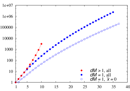
Figure 2: (Color online) The number of diagrams contributing to a given level illustrates the rise in complexity with increasing $p$. Systems fall into one of two classes of complexity: the more complex ones with $dM>1$ (top curve) and the less complex ones with $dM=1$ (middle curve). In addition, the bottom curve gives the number of velocity independent diagrams for $dM=1$.

As in the case of one-dimensional systems, the obtained discretized effective actions can be applied to a host of relevant physical many-body problems in the framework of the Path Integral Monte Carlo approach, including the continuous-space worm algorithm boninsegni . For instance, our approach is applicable to efficiently determine the statistical properties of Bose-Einstein condensates which are confined in harmonic or anharmonic traps dalibard2004 ; dalibard2005 ; pelster2007 ; progress . Furthermore, our method is ideally suited for dealing with dilute quantum gases in a disorder environment where the impact of two-particle interactions upon the recently discovered phenomenon of Anderson localization is at present studied anderson1 ; anderson2 .

VI Conclusions

We have given a detailed presentation of an analytic procedure for determining the short-time propagation of a general non-relativistic $M$-particle theory in $d$ dimensions to extremely high orders. The procedure is based on recursively solving the Schrödinger equation for the transition amplitude in a power series of the propagation time. This leads to a new recursion relation that has been solved to order $p=10$ for the case of a general many-body theory. For a single particle moving in a general potential in $d=1$ we have even achieved $p=35$. In addition, for specific classes of potentials as, for instance, polynomial potentials, the equations have been solved to order $p=140$. The resulting Schwinger-Dyson equation and its recursive solution have also been cast both in a familiar diagrammatic and a compact topological notation. The presented results define the state-of-the-art for calculating short-time expansion amplitudes. They can be used to obtain orders of magnitude speedup in Path Integral Monte Carlo calculations. Thus, the extremely high orders of the short-time expansion make it possible to perform new and precise analytical calculations of thermodynamical and dynamical properties of many-body systems. A list of applications of the presented method to relevant physical systems is briefly outlined.

References

- (1) R. P. Feynman, Rev. Mod. Phys. 20, 367 (1948).
- (2) R. P. Feynman, and A. R. Hibbs, Quantum Mechanics and Path Integrals, McGraw-Hill, New York, 1965.
- (3) R. P. Feynman, Statistical Mechanics, W. A. Benjamin, New York, 1972.
- (4) H. Kleinert, Path Integrals in Quantum Mechanics, Statistics, Polymer Physics, and Financial Markets, 4th edition, World Scientific, Singapore, 2006.
- (5) D. M. Ceperley, Rev. Mod. Phys. 67, 279 (1995).
- (6) S. Pilati, K. Sakkos, J. Boronat, J. Casulleras, and S. Giorgini, Phys. Rev. A 74, 043621 (2006).
- (7) C. Zhang, K. Nho, and D. P. Landau, Phys. Rev. A 77, 025601 (2008).
- (8) S. Pilati, S. Giorgini, and N. Prokof’ev, Phys. Rev. Lett. 100, 140405 (2008).
- (9) E. Vitali, M. Rossi, F. Tramonto, D. E. Galli, and L. Reatto, Phys. Rev. B 77, 180505(R) (2008).
- (10) D.-H. Kim, Y.-C. Lin, and H. Rieger, Phys. Rev. E 75, 016702 (2007).
- (11) C. Predescu, Phys. Rev. E 69, 056701 (2004).
- (12) A. Bogojević, A. Balaž, and A. Belić, Phys. Rev. Lett. 94, 180403 (2005).
- (13) A. Bogojević, A. Balaž, and A. Belić, Phys. Rev. B 72, 064302 (2005).
- (14) A. Bogojević, A. Balaž, and A. Belić, Phys. Lett. A 344, 84 (2005).
- (15) A. Bogojević, A. Balaž, and A. Belić, Phys. Rev. E 72, 036128 (2005).
- (16) A. Bogojević, I. Vidanović, A. Balaž, and A. Belić, Phys. Lett. A 372, 3341 (2008).
- (17) C. M. Bender and T. T. Wu, Phys. Rev. 184, 1231 (1969); Phys. Rev. D 7, 1620 (1973).
- (18) W. Janke and H. Kleinert, Phys. Rev. Lett. 75, 2787 (1995).
- (19) F. Weissbach, A. Pelster, and B. Hamprecht, Phys. Rev. E 66, 036129 (2002).
- (20) S.F. Brandt, H. Kleinert, and A. Pelster, J. Math. Phys. 46, 032101 (2005).
- (21) J. Dreger, A. Pelster, and B. Hamprecht, Europ. Phys. J. B 45, 355 (2005).
- (22) M. Bachmann, H. Kleinert, and A. Pelster, Phys. Rev. D 61, 085017 (2000).
- (23) H. Kleinert, A. Pelster, B. Kastening, and M. Bachmann, Phys. Rev. E 62, 1537 (2000).
- (24) H. Kleinert, A. Pelster, and B. Van den Bossche, Physica A 312, 141 (2002).
- (25) A. Pelster, H. Kleinert, and M. Bachmann, Ann. Phys. (N.Y.) 297, 363 (2002).
- (26) A. Pelster and K. Glaum, Phys. Stat. Sol. B 237, 72 (2003).
- (27) A. Pelster and H. Kleinert, Physica A 323, 370 (2003).
- (28) http://www.wolfram.com
- (29) http://scl.phy.bg.ac.yu/speedup
- (30) E. L. Pollock and D. M. Ceperley, Phys. Rev. B 30, 2555 (1984).
- (31) A. Sethia, S. Sanyal, and Y. Singh, J. Chem. Phys. 93, 7268 (1990).
- (32) A. Sethia, S. Sanyal, and F. Hirata, Chem. Phys. Lett. 315, 299 (1999).
- (33) http://smc.vnet.net/mathtensor.html
- (34) M. Boninsegni, N. Prokof’ev, and B. Svistunov, Phys. Rev. Lett. 96, 070601 (2006).
- (35) V. Bretin, S. Stock, Y. Seurin, and J. Dalibard, Phys. Rev. Lett. 92, 050403 (2004).
- (36) S. Stock, B. Battelier, V. Bretin, Z. Hadzibabic, and J. Dalibard, Laser Phys. Lett. 2, 275 (2005).
- (37) S. Kling and A. Pelster, Phys. Rev. A 76, 023609 (2007).
- (38) A. Balaž, A. Bogojević, I. Vidanović, and A. Pelster, in preparation.
- (39) J. Billy, V. Josse, Z.C. Zuo, A. Bernard, B. Hambrecht, P. Lugan, D. Clement, L. Sanchez-Palencia, P. Bouyer, and A. Aspect, Nature 453, 891 (2008).
- (40) G. Roati, C. D’Errico, L. Fallani, M. Fattori, C. Fort, M. Zaccanti, G. Modugno, M. Modugno, and M. Inguscio, Nature 453, 895 (2008).