IDLA on the Supercritical Percolation Cluster

Abstract.

We consider the internal diffusion limited aggregation (IDLA) process on the infinite cluster in supercritical Bernoulli bond percolation on $\mathbb{Z}^{d}$. It is shown that the process on the cluster behaves like it does on the Euclidean lattice, in that the aggregate covers all the vertices in a Euclidean ball around the origin, such that the ratio of vertices in this ball to the total number of particles sent out approaches one almost surely.

1. Introduction

1.1. Background and discussion

Given a graph, IDLA defines a random aggregation process, starting with a single vertex and growing by a vertex in each time step. To begin the process, we specialize a vertex $v$ to be the initial aggregate on the graph. In each time step, we send out one random walk from $v$. Once this walk exits the aggregate, it stops, and the new vertex is added to the aggregate. Let $\mathcal{I}(n)$ be the aggregate in step $n$, thus $\mathcal{I}(1)=\left\{v\right\}$ and $\left|\mathcal{I}(n)\right|=n$.

This process is a special case of a model Diaconis and Fulton introduced in [6]. In the setting where the graph is the $d$-dimensional lattice, Lawler, Bramson and Griffeath in [10] used Green function estimates to prove the process has a Euclidean ball limiting shape. Let $B_{r}$ be all vertices in $\mathbb{Z}^{d}$ of Euclidean distance less than $r$ from the origin. The main theorem in [10] implies that for any $\epsilon>0$, $\mathcal{I}(\left|B_{R}\right|)\supset B_{(1-\epsilon)R}$ for all sufficiently large $R$ with probability one. Seeking to generalize this result to other graphs, we note that convergence of a random walk on the lattice to isotropic Brownian motion plays an important role in convergence of IDLA on the lattice to an isotropic limiting shape.

However, this property by itself is in general not enough for IDLA to have such an inner bound, as the following example shows. Consider the three dimensional Euclidean lattice, and choose a vertex $v$ at distance $R$ from the origin. Let $r=R^{0.9}$ and let $B_{r}(v)$ be the set of vertices of distance less than $r$ from $v$. Remove all edges but one from the boundary of $B_{r}(v)$, and denote by $v^{\prime}$ the only vertex in $B_{r}(v)$ with a neighbor outside of $B_{r}(v)$. Let us look at $\mathcal{I}(\left|B_{2R}\right|)$. A rough calculation gives that the average number of visits to $v^{\prime}$ is of order $R^{-1}\left|B_{2R}\right|$. Since at least $\left|B_{r}(v)\right|=R^{2.7}$ visits to $v^{\prime}$ are needed to fill $B_{r}(v)$, we don’t expect the ball to be full after an order of $R^{3}$ particles have been sent out. Repeating this edge removal procedure for balls of radius $R_{n}^{0.9}$ at distance $R_{n}$ from the origin where $R_{n}=2^{n}R$, will ensure that there is never a Euclidean inner bound. However, a random walk from the origin on this graph will converge to Brownian motion because our disruptions are sublinear. We will not give full proofs of these facts, but hope they convince the reader that to get an inner bound some kind of local regularity property is needed.

The main theorem of this paper states that IDLA on the supercritical cluster in the lattice has a Euclidean ball as an inner bound. The two main tools that are used to show this are a quenched invariance principle [3] which gives us convergence in distribution to Brownian Motion from a fixed point, and a Harnack inequality from [2], which give us oscillation bounds on harmonic functions in all small balls close to the origin. The latter allows us to establish the local regularity missing from the above example.

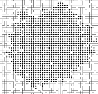
Figure 1.1. IDLA of 1000 particles from marked vertex on the percolation cluster with $p=0.7$.

1.2. Assumptions and statement

Consider supercritical bond percolation in $\mathbb{Z}^{d}$ with the origin conditioned to be in the infinite cluster. Let the graph $\Gamma(V,E)$ be the natural embedding in $\mathbb{R}^{d}$ of the infinite cluster, i.e. $V\subset\mathbb{R}^{d}$. Fixing this embedding for $\Gamma$, we get two separate (but comparable, see [1]) distances. We denote by $\left|x-y\right|$ or $d(x,y)$ Euclidean distance between points $x,y$, and by $d_{\Gamma}(x,y)$ the graph distance between them. If one of the points is not in $V$, $d_{\Gamma}(x,y)=\infty$. Let $B_{r}(x)=\{v\in V\ |\ d(x,v)<r\}$ be the vertices contained in a Euclidean ball of radius $r$ and center $x$. We abbreviate $B_{r}(\mathbf{0})$ as $B_{r}$. To differentiate between such a set of vertices and a full ball in $\mathbb{R}^{d}$, we denote by bold lowercase the following: $\mathbf{b}_{r}(x)=\{y\in\mathbb{R}^{d}\ |\ d(x,y)<r\}$. Let $\mathbf{d}_{r}(x)$ be a box of side $r$ with center $x$, and as above, let $D_{r}(x)$ be the vertices in this box.

By existing work, which we will reference later, we know that with probability one, the graph of the supercritical cluster, $\Gamma$, in its natural $\mathbb{R}^{d}$ embedding, satisfies the following assumptions:

1. A random walk on $\Gamma$ converges weakly in distribution to a Brownian Motion as defined in 1.4.

2. Convergence to vertex density $a_{G}>0$ as defined in 1.5.

3. A uniform upper bound on exit time from a ball as defined in 1.6.

4. A Harnack inequality as defined in 1.7.

We denote by $X_{t}$ a discrete “blind” random walk on $\Gamma$ defined as follows. For $x\in\Gamma$ and $t\in\mathbb{N}\cup\left\{0\right\}$, $P\left(X_{t+1}=y|X_{t}=x\right)=1/2d$ if $y$ is a neighbor of $x$ in $\Gamma$, and $P\left(X_{t+1}=x|X_{t}=x\right)=1-\deg x/2d$. We prefer this walk since its Green functions are symmetric, a fact which will be useful later on. For non-integer $t$ we set $X_{t}=X_{\lfloor t\rfloor}$.

Note that assumption 4 does not imply 3, see [5] for a counterexample.

Using only above assumptions and that $V\subset\mathbb{Z}^{d}$ (which serves mostly to simplify notation and could be replaced by weaker conditions), we show the IDLA process starting at $\mathbf{0}$ will have a Euclidean ball inner bound as stated in the following theorem:

Let $\mathcal{I}(n)$ denote the random IDLA aggregate of $n$ particles starting at $\mathbf{0}$.

Theorem 1.1.

Almost surely, for any $\epsilon>0$, we have that for all large enough $R$, $B_{(1-\epsilon)R}\subset\mathcal{I}(\left|B_{R}\right|)$

We fix $\epsilon$ with which we prove the above for the rest of the paper.

1.3. Outline

In the remainder of this section we state our assumptions precisely, and explain why these assumptions are valid almost surely for the infinite cluster in supercritical percolation.

Then, to prove IDLA inner bound, we need to show that for each vertex $v\in V$ the Green function from $\mathbf{0}$ and expected exit time from a ball around 0 of a random walk starting at $v$, behave similarly to those functions of a Brownian motion. The exact statement needed appears in Lemma 3.1. The invariance principle gives us integral convergence of these functions to the right value, but to improve them to pointwise statements, we must show that they are locally regular. We use the Harnack inequality from [2] to prove they are Hölder continuous. This is a similar scheme to improving a CLT to an LCLT, as was done in [4] using a different method than ours.

In section 2, we start by proving a lemma comparing expected exit time from a set to the Green function of a point in the set. Then, we show how our Harnack assumption leads to an oscillation inequality which we use to show regularity of the Green function and expected exit time of the walk in a ball when we are far from the boundary and the center. Next, in section 3, we use our assumption of an invariance principle to show that in small balls the integral of these functions approaches a tractable limit that can be calculated by knowledge of Brownian motion. Finally, in section 4, we utilize these estimates to prove theorem 1.1.

Remark 1.2.

Since the paper makes use of results based on ergodic theory, there is no rate estimate for the convergence in theorem 1.1. Also, on the Euclidean lattice there is an almost sure outer bound with sublinear fluctuations from the sphere. Another interesting question that is not treated here, is whether a similar outer bound holds in our setting.

1.4. Weak convergence to Brownian Motion

In this and the next three subsections, we give a precise formulation of each of our assumptions from above, and argue that they hold a.s. on $\Gamma$, the supercritical cluster.

Let $\mathcal{C}_{T}^{d}=C([0,T]\to\mathbb{R}^{d})$, i.e. the continuous functions from the closed interval $[0,T]$ to $d$-dimensional Euclidean space. For $R\in\mathbb{N}$, let

$$w_{R}(t)=\frac{1}{R}\left(X_{\lfloor tR^{2}\rfloor}+(tR^{2}-\lfloor tR^{2}\rfloor)(X_{\lfloor tR^{2}\rfloor+1}-X_{\lfloor tR^{2}\rfloor})\right).$$

Thus $w_{R}(t)$ is a scaled linear interpolation of $X_{t}$ (defined in 1.2) with its restriction to $[0,T]$ an element of $\mathcal{C}_{T}^{d}$.

We say that assumption 1 holds if for any $T>0,$ the law of $w_{R}(t)$ on $\mathcal{C}_{T}^{d}$ converges weakly in the supremum topology to the law of a (not necessarily standard) Brownian Motion $(B_{t}:0\leq t\leq T)$ .

Lemma 1.3.

Assumption 1 holds for $\Gamma$ with probability one.

Proof.

This is Theorem 1.1 in [3]. Another paper with a similar invariance principle is [11]. ∎

Let $\mathcal{B}(t)$ denote the Brownian motion weak limit of $X_{t}$.

1.5. Convergence to positive density

Assumption 2 holds if there exists a positive $a_{G}$ such that for any $\delta,\gamma>0$ and all sufficiently large $R$ we have that for all $x\in\mathbf{b}_{R}$ and all $\delta R\leq r\leq R$

$$\ \ \biggl{|}\frac{|D_{r}(x)|}{r^{d}}-a_{G}\biggr{|},\ \biggl{|}\frac{|B_{r}(x)|}{\left|\mathbf{b}_{1}\right|r^{d}}-a_{G}\biggr{|}<\gamma.$$

That is, balls and boxes of size $\delta R$ to $R$, have vertex density in $\left(a_{G}-\gamma,a_{G}+\gamma\right)$ for all large enough $R$.

Lemma 1.4.

Assumption 2 holds for $\Gamma$ with probability one.

Proof.

Let $\theta(p)$ be the probability for $\mathbf{0}$ to be in the infinite cluster. $\theta(p)$ is positive in the supercritical regime. From Theorem 3 in [8] for $d=2$ and from (2) on p. 15 of [9] for $d>2$, we know that for any $\rho>0$ there is a positive $c=c(\rho)$ such that

$$P\left(n^{-d}\left|D_{n}(x)\right|<(1-\rho)\theta(p)\right)<\exp(-cn).$$

where $x\in\mathbb{R}^{d}$ and $n\in\mathbb{N}$. Recall $D_{n}(x)$ are the vertices in a box of side-length $n$ and center $x$. Theorem 2 in [8] proves the easier density upper bound for $d=2$, which under trivial modifications gives that for all $d$

$$P\left(n^{-d}\left|D_{n}(x)\right|>(1+\rho)\theta(p)\right)<\exp(-cn).$$

The above, together with Borel Cantelli gives that if we choose $\gamma>0$, $x\in\mathbf{b}_{1}$, then for all large enough $R$

$$\left|\left|D_{\rho R}(Rx)\right|-\theta(p)(\rho R)^{d}\right|<\frac{\gamma}{2}R^{d}.$$

So we have the result for small boxs of size $\rho R$. To expand it to larger boxes, let $D$ be any box of diameter between $\delta R$ to $R$. We partition the box $D_{R}$ into $\rho R$-sized boxes and choose $\rho=\rho(\delta)$ small enough so that the number of boxes that intersect both $D$ and $D_{R}\backslash D$ is negligible compared to the number that intersect $D$. Proving for balls is similar. ∎

1.6. Uniform Bound on Exit time from ball

Denote by $\tau_{r}(x)$ the first time the walk leaves $B_{r}(x)$, and write $\tau_{r}$ for $\tau_{r}(\mathbf{0})$.

Assumption 3 holds if there is a $c_{E}$ such that for any $\delta>0$ and all large enough $R$, if $x\in B_{R}$ and $r>\delta R$ then

(1.1) $$E_{x}\left[\tau_{r}(x)\right]<c_{E}r^{2}.$$

The assumption holds for $\Gamma$ with probability one as a direct consequence of the following lemma, proved below.

Lemma 1.5.

With probability one, there is an $L$ such that for all $\delta>0$ and all large enough $R$, if $x\in B_{R}$ and $r>\delta R$ then

(1.2) $$P_{x}(\tau_{r}(x)>Lr^{2})<\exp(-cL).$$

Proof.

Since we prove for all $R$ outside a bounded interval, it suffices to prove the above for $r=\delta R$ with fixed $\delta>0$. To prove this holds a.s. for supercritical percolation clusters, we use a heat kernel upper bound given in Theorem 1 of Barlow’s paper [2]. The proof in [2] is for continuous walks with a mean time of one between jumps. However, it can be transferred to our discrete walk using Theorem 2.1 of [3]. We state an implication of what was proved.

With probability one there exists a function from $V$ to $\mathbb{N}$, $\left\{\mathcal{T}_{x}<\infty\right\}_{x\in V}$ where $\mathcal{T}_{x}$ is sublinear in the sense that $\frac{\mathcal{T}_{x}}{\|x\|}\to 0$, and there exist positive constants $c_{1},c_{2}$ such that for any $x\in V$, the following holds. For all $y\in B_{t}(x),\ t\geq\mathcal{T}_{x}$:

(1.3) $$P_{x}(X_{t}=y)<c_{2}t^{-d/2}.$$

Barlow’s result actually states that almost surely $\mathcal{T}_{x}$ grows slower than a logarithmic function of $\|x\|$ and gives stronger Gaussian bounds for the heat kernel from below and above.

Using the heat kernel upper bound (1.3), the convergence to zero of $\frac{\mathcal{T}_{x}}{\|x\|}$, and the upper bound on vertex density resulting from $\Gamma\subset\mathbb{Z}^{d}$, we have that for any $K$ and all large enough $R$, if $x\in B_{R}$ and $r=\delta R$, then

$$P_{x}(X_{Kr^{2}}\notin B_{r}(x)) = 1-\sum_{y\in B_{r}(x)}P_{x}(X_{Kr^{2}}=y)$$

$$\geq 1-\sum_{y\in B_{r}(x)}c_{2}K^{-d/2}r^{-d}$$

$$\geq 1-C(d)K^{-d/2}.$$

Thus for some $K^{\prime}$, for all large enough $R$, and all $x\in B_{R}$, $P_{x}(X_{K^{\prime}r^{2}}\in B_{r}(x))<\frac{1}{2}$. Next, for any positive $L$, we use the Markov property to upper bound $P_{x}(\tau_{r}(x)>LK^{\prime}r^{2})$ by

$$P_{x}(X_{K^{\prime}r^{2}}\in B_{r}(x))\prod_{i=2}^{\lfloor L\rfloor}P(X_{iK^{\prime}r^{2}}\in B_{r}(x)\ |\ X_{(i-1)K^{\prime}r^{2}}\in B_{r}(x))\leq 2^{-\lfloor L\rfloor},$$

which proves the claim. ∎

We will later use that assumption 3 implies $L_{1}$ convergence of $R^{-2}\tau_{R}\wedge T$ to $R^{-2}\tau_{R}$ with $T$, uniformly in $R$ for all $x\in B_{R}$.

Lemma 1.6.

For all $\beta>0$ there is a $T(\beta)$ such that for all large enough $R$, $\forall x\in B_{R}$

(1.4) $$\left|E_{x}\left[\tau_{R}\right]-E_{x}\left[\tau_{R}\wedge TR^{2}\right]\right|<\beta R^{2}.$$

We rewrite the left hand side of (1.4) and use the Markov property with the exit time assumption.

$$E_{x}\left[\left(\tau_{R}-TR^{2}\right)\mathbf{1}_{\left\{\tau_{R}>TR^{2}\right\}}\right] = \sum_{y\in B_{R}}\biggl{[}E_{x}\left[\tau_{R}-TR^{2}\ |\ \tau_{R}>TR^{2},X(TR^{2})=y\right]\cdot$$

$$P(\tau_{R}>TR^{2},X(TR^{2})=y)\biggr{]}$$

$$= \sum_{y\in B_{R}}E_{y}\left[\tau_{R}\right]P(\tau_{R}>TR^{2},X(TR^{2})=y)$$

$$\leq c_{E}R^{2}\sum_{y\in B_{R}}P(\tau_{R}>TR^{2},X(TR^{2})=y)$$

$$= c_{E}R^{2}P(\tau_{R}>TR^{2}).$$

Since $E_{x}\left[\tau_{R}/R^{2}\right]$ is bounded by $c_{E}$ for all $R$, we have by the Markov inequality that $P(\tau_{R}/R^{2}>T)\leq c_{E}/T$ which converges to zero as $T$ goes to $\infty$ uniformly in $R$ for all $x\in B_{R}$.

1.7. Harnack inequality

A function $h:\Gamma\to\mathbb{R}$ is harmonic on $x\in\Gamma$ if $h(x)=\left|N(x)\right|^{-1}\sum_{y\in N(x)}h(y)$ where $N(x)=\left\{y\in\Gamma:d_{\Gamma}(x,y)=1\right\}$ are the neighbors of $x$. We say $h$ is harmonic on $Z\subset\Gamma$ if it harmonic on every vertex $v\in Z$.

Assumption 4 holds if there is a $1<c_{H}<\infty$ such that for all $\delta>0$ we have that for all large enough $R$, if $x\in B_{R}$, $r>\delta R$ and $h$ is a function that is non-negative and harmonic on $B_{2r}(x)$ then

(1.5) $$\sup_{B_{r}(x)}h\leq c_{H}\inf_{B_{r}(x)}h.$$

In order to simplify the paper, the inequality above is formulated for Euclidean distance rather than graph distance. We show that since the distances are almost surely comparable on $\Gamma$, this is the same. We start by proving the assumption holds for graph distance, using Lemma 2.19 and Theorem 5.11 of [2]. We write $B_{r}^{\Gamma}=\left\{x\in\Gamma:d_{\Gamma}(\mathbf{0},x)\leq r)\right\}$. The lemma, using appropriate parameters and Borel Cantelli, tells us that for all large enough $R$, $B_{R\log R}^{\Gamma}$ are very good balls. Specifically, all balls contained in $B_{R\log R}^{\Gamma}$ of graph radius larger than $R^{1/4(d+2)}$ have a positive volume density and satisfy a weak Poincaré inequality as explained in (1.15) and (1.16) of the same. Theorem 5.11 then tells us that for very good ball of graph radius $R\log R$, all $x\in B_{\left(R\log R\right)/3}^{\Gamma}$ satisfy that for any function $h$ non-negative harmonic on $B_{R}^{\Gamma}(x)$

(1.6) $$\sup_{B_{R/2}^{\Gamma}(x)}h\leq\hat{c}_{H}\inf_{B_{R/2}^{\Gamma}(x)}h$$

where $\hat{c}_{H}(d,p)>0$ is a constant dependent only on dimension and percolation probability. Since all but a finite number of balls of graph radius $R\log R$ are very good and $R$ is $o(R\log R)$ we have assumption 4 for graph distance.

Next, we transfer this to the Euclidean balls formulation of (1.5). By Theorem 1.1 of [1], we have that for some $k>0$, $\rho(d,p)>0$ and $M<\infty$,

$$\mathbb{P}\left[d_{\Gamma}(x,y)>\rho m\Bigl{|}x,y\in\Gamma,\left|x-y\right|=m>M\right]<\exp(-km).$$

Let $A(x,y)$ be the event $\left\{d_{\Gamma}(x,y)>\rho m\right\}$. Union bounding the probability for $A(x,y)$ over every pair of points in $B_{R}$ of Euclidean distance greater than $c\log R$ for some large $c(k)$, we upper bound the probability of any such event occuring by

$$CR^{d}\sum\limits_{m=c\log R}^{\infty}m^{d-1}\exp(-km)<C^{\prime}R^{d}\left(\log R\right)^{d-1}R^{-2d},$$

which is summable for $d>1$. Hence by Borel Cantelli, almost surely for all large enough $R$, we have that for any $x,y\in B_{R}$ with $\left|x-y\right|>c\log R$, $d_{\Gamma}(x,y)<\rho\left|x-y\right|$. Since $\log R$ is $o(R)$, this implies that for any $\delta>0$ and all large enough $R$, for any $x\in B_{R}$,

(1.7) $$B_{\delta\rho^{-1}R}(x)\subset B_{\delta R}^{\Gamma}(x).$$

Note that $B_{r}^{\Gamma}(x)\subset B_{r}(x)$ always because $\Gamma$ is embedded in $\mathbb{Z}^{d}$. Hence, given a function that is non-negative harmonic on $B_{2r}(x)$ it is also such on $B_{2r}^{\Gamma}(x)$. For large enough $R$, we use (1.6) and (1.7) to get (1.5) for $B_{\rho^{-1}r}(x)$ with constant $\hat{c}_{H}$. A routine chaining argument (see e.g. (3.5) in [5]) transfers this to $B_{r}(x)$ as required with new constant $c_{H}$.

2. Pointwise bounds on Green function and expected exit time

In this section, we show the assumptions of a uniform bound on exit time from a ball along with the Harnack inequality give us pointwise bounds of the Green function and expected exit time of a random walk.

As a convention, we use plain $c$ and $C$ to denote positive constants that do not retain their values from one expression to another, as opposed to subscripted constants $c_{i},$ that do. In general, these constants are graph dependent, and in the context of percolation, can be seen as random functions of the percolation configuration. However, we view the graph as being fixed and satisfying the assumptions stated in subsection 1.2.

We start with a general lemma on the relation between expected exit time from a set and the expected number of visits to a fixed point in the set.

Let $Z\subset\Gamma$ and let $\tau_{Z}$ be the first hitting time of $Z$ for $X_{t}$. For $x\in\Gamma$ we set $G_{Z}(x)=E_{x}\left[\sum_{t=0}^{\tau_{Z}}\mathbf{1}_{\left\{X_{t}=x\right\}}\right]$, the expected number of visits to $x$ of a walk starting at $x$ before $\tau_{Z}$.

Lemma 2.1.

There is a $k=k(d)>0$ such that for any $x\in\Gamma$ and $Z\subset\Gamma$ where $N(x)\cap Z=\emptyset$

(2.1) $$E_{x}\left[\tau_{Z}\right]>kG_{Z}^{2}/\log G_{Z}.$$

Proof.

Recall from 1.2 that $X_{t}$ has a positive staying probability at certain vertices. Since we apply electrical network interpretation to estimate hitting probabilities, we prove the above for $Y_{t}$, the usual discrete simple random walk, with $0$ probability to stay at a vertex. This implies (2.1) for $X_{t}$ as well, since the expected exit time cannot decrease, and the Green functions for $X_{t}$ can only grow by a $2d$ factor since the escape probabilites for $X_{t}$ and $Y_{t}$ are at most a $2d$ factor apart.

Fix $x\in\Gamma$, set $T_{0}=0$, and define for each $i\in\mathbb{N}$ the r.v.’s

$$T_{i}=\inf\left\{t>T_{i-1}:Y_{t}=x\right\}.$$

Let $i^{*}=\inf\left\{i:T_{i}=\infty\right\}$. For $1\leq i\leq i^{*}$ let $\rho_{i}=T_{i}-T_{i-1}$. We show there are positive constants $k_{1},k_{2}$ dependent only on $d$ such that

(2.2) $$P\left[\rho_{1}\geq k_{1}r^{2}/\log r\right]\geq\frac{k_{2}}{r}.$$

For some $r>1$, let $\partial B_{r}^{\Gamma}(x)=\left\{v\in\Gamma:d_{\Gamma}(v,x)=r\right\}$. By electrical network interpretation (see e.g. [7]), the probability for a walk beginning at $x$ to hit $\partial B_{r}^{\Gamma}(x)$ before returning to $x$ is $(2d)^{-1}C_{eff}(r)$, where $C_{eff}(r)$ is the effective conductance from $x$ to $\partial B_{r}^{\Gamma}(x)$. Since $\Gamma$ is infinite and connected, for any $r$ there is a connected path of $r$ edges from $x$ to $\partial B_{r}^{\Gamma}(x)$. By the monotonicity principle, $C_{eff}(r)$ is at least the conductance on this path, which is $r^{-1}$. Thus the probability to hit some $y\in\partial B_{r}^{\Gamma}(x)$ before returning to $x$ is at least $\left(2dr\right)^{-1}$.

Next, let $y\in\partial B_{r}^{\Gamma}(x)$. By the Carne-Varopoulos upper bound (see [13]),

$$P\left[Y_{t}=x|Y_{0}=y\right]\leq 4d^{1/2}\exp\left(-\frac{r^{2}}{2t}\right)$$

and thus, for some $k_{1}(d),k_{2}(d)>0$ and all $r>1$, the probability that a walk starting at $y\in\partial B_{r}^{\Gamma}(x)$ does not hit $x$ in the next $\lfloor k_{1}r^{2}/\log r\rfloor$ steps, by union bound, is greater than $k_{2}$. Together with our lower bound on the probability that we arrive at such a $y\in\partial B_{r}^{\Gamma}(x)$, we get (2.2).

Next, let $g=\inf\left\{i:T_{i}>\tau_{Z}\right\}$ be the number of visits of $Y_{t}$ to $x$ before hitting $Z$, including $t=0$ . $g$ is a geometric random variable with mean $G=G_{Z}$. Let $\alpha=\frac{1}{2}\ln\left(4/3\right)$ and note that since there is a constant in (2.1) and $\tau_{Z}\geq 1$, we can assume $G>2$. Thus

$$P\left[g\geq\alpha G\right] \geq \left(1-G^{-1}\right)^{\alpha G}$$

$$\geq \left(1-G^{-1}\right)^{2\alpha\left(G-1\right)}$$

$$\geq e^{-2\alpha}=3/4$$

We further assume $G>\frac{2}{\alpha}\vee\frac{16}{k_{2}}$ so that $\alpha G-1>\alpha G/2$ and $G\frac{k_{2}}{16}>1$. Let $A$ be the event that there is an $1\leq i\leq\left(\alpha G-1\right)\wedge i^{*}$ such that $\rho_{i}>k_{1}\left(\frac{k_{2}}{16}G\right)^{2}/\log\left(\frac{k_{2}}{16}G\right)$ Note that $i^{*}\leq\alpha G-1$ implies $A$. Thus by (2.2) and the independence of consecutive excursions from $x$,

$$P\left[A^{c}\right]\leq\left(1-\frac{16}{G}\right)^{\alpha G/2}\leq e^{-8\alpha}$$

which is smaller than $1/4$.

Thus

$$P\left[\left\{g\geq\alpha G\right\},A\right]\geq\frac{1}{2}.$$

This implies the lemma since $\tau_{Z}>\sum_{i=1}^{g-1}\rho_{i}$, and for $k=k_{1}k_{2}^{2}/256$, $\sum_{i=1}^{g-1}\rho_{i}>kG^{2}/\log G$. ∎

Next, we state the fact that a Harnack inequality implies an oscillation inequality. For a set of vertices $U$ and a function $u$, let

$$\mbox{osc}_{U}(u)=\max\nolimits_{U}(u)-\min\nolimits_{U}(u).$$

Proposition 2.2.

Let $x\in\Gamma$ and assume that for some $r>0$ we have that any function $h$ that is non-negative and harmonic on $B_{2r}(x)$ satisfies (1.5) on $B_{r}(x)$. Then for any $h$ that is harmonic on $B_{2r}(x)$, we have

(2.3) $$\mbox{osc}_{B_{r}(x)}h\leq\frac{c_{H}-1}{c_{H}+1}\mbox{osc}_{B_{2r}(x)}h.$$

Proof.

We quote a proof from chapter 9 of [12].

Set $v=h-\min_{B_{2r}(x)}h$. Since $v$ is non-negative and harmonic on $B_{2r}(x)$, the Harnack inequality (1.5) is satisfied here, so we have

$$\max_{B_{r}(x)}v\leq c_{H}\min_{B_{r}(x)}v,$$

whence

$$\max_{B_{r}(x)}h-\min_{B_{2r}(x)}h\leq c_{H}\left(\min_{B_{r}(x)}h-\min_{B_{2r}(x)}h\right),$$

and

$$\mbox{osc}_{B_{r}(x)}h\leq\left(c_{H}-1\right)\left(\min_{B_{r}(x)}h-\min_{B_{2r}(x)}h\right).$$

Similarly, we have

$$\mbox{osc}_{B_{r}(x)}h\leq\left(c_{H}-1\right)\left(\max_{B_{2r}(x)}h-\max_{B_{r}(x)}h\right).$$

Summing up these two inequalities, we obtain

$$\mbox{osc}_{B_{r}(x)}h\leq\frac{1}{2}\left(c_{H}-1\right)\left(\mbox{osc}_{B_{2r}(x)}h-\mbox{osc}_{B_{r}(x)}h\right),$$

whence (2.3) follows. ∎

Iterating this on the Harnack assumption 4 we get

Corollary 2.3.

For any $\alpha>0$ there is an $M(\alpha)$ such that for any $\eta>0$ and for all $R>R_{\eta}$, if $x\in B_{R}$, $r\geq\eta R$ and $h$ is a harmonic function on $B_{M(\alpha)r}(x)$ then

$$\mbox{osc}_{B_{r}(x)}h\leq\alpha\mbox{osc}_{B_{Mr}(x)}h.$$

We use this to show regularity of the green function and for expected exit time.

Lemma 2.4.

There is a $c_{G}(\epsilon)$ such that for all large enough $R$, and any $x\in B_{(1-\epsilon)R}\setminus B_{\epsilon R}$

(2.4) $$G_{\tau_{R}}(\mathbf{0},x)<c_{G}R^{2-d}.$$

Proof.

Any two vertices in $u,v\in B_{(1-\epsilon)R}\setminus B_{\epsilon R}$ can be joined by a path of $n<C(d)/\epsilon$ overlapping balls $B_{\epsilon/4}(x_{1}),\ldots,B_{\epsilon/4}(x_{n})$ that are all subsets of $B_{(1-\epsilon/2)R}\setminus B_{\left(\epsilon/2\right)R}$ such that $x_{1}=u$ and $x_{n}=v$. Since $G_{\tau_{R}}(\mathbf{0},x)$ is positive and harmonic in $B_{(1-\epsilon/2)R}\setminus B_{\left(\epsilon/2\right)R}$, Harnack assumption 4 tells us that $c_{H}^{-C/\epsilon}<u/v<c_{H}^{C/\epsilon}$. Next, note that $\sum_{x\in B_{R}}G_{\tau_{R}}(\mathbf{0},x)=E_{\mathbf{0}}\left[\tau_{R}\right]$. Thus, letting $M(R)=\max\left\{G_{\tau_{R}}(\mathbf{0},x):x\in B_{(1-\epsilon)R}\setminus B_{\epsilon R}\right\}$, and using the exit time bound in assumption 3, we get

$$\left|B_{R}\right|c_{H}^{-C/\epsilon}M\leq\sum_{x\in B_{R}}G_{\tau_{R}}(\mathbf{0},x)<c_{E}R^{2}.$$

∎

Lemma 2.5.

For any $\beta>0$, there is a $\delta>0$ such that for all large enough $R$, any $x,y\in B_{(1-\epsilon)R}\setminus B_{\epsilon R}$ satisfying $\left|x-y\right|<\delta R$ also satisfy

(2.5) $$\biggl{|}G_{\tau_{R}}(\mathbf{0},x)-G_{\tau_{R}}(\mathbf{0},y)\biggr{|}\leq\beta R^{2-d}.$$

Proof.

$G_{\tau_{R}}(\mathbf{0},x)$ is positive and harmonic in $B_{(1-\epsilon/2)R}\setminus B_{\left(\epsilon/2\right)R}$ and bounded by $c_{G}R^{2-d}$. We use corollary 2.3 with $\alpha=\beta c_{G}^{-1}$ and $\eta=\epsilon/\left(2M(\alpha)\right)$. This gives us the lemma with $\delta=\eta$.∎

Lemma 2.6.

For any $\beta>0$, there is a $\delta>0$ such that for all large enough $R$, any $x,y\in B_{(1-\epsilon)R}$ satisfying $\left|x-y\right|<\delta R$ also satisfy:

(2.6) $$\biggl{|}E_{x}\left[\tau_{R}\right]-E_{y}\left[\tau_{R}\right]\biggr{|}\leq\beta R^{2}.$$

Proof.

Fix $x\in B_{(1-\epsilon)R}$ and for $\delta>0$ determined below, fix some $y\in B_{\delta R}(x)$. Define the r.v. $\tau_{1}$ to be the random time it takes a walk starting somewhere inside $B_{\epsilon R}(x)$ to exit $B_{\epsilon R}(x)$, and let $\tau_{2}=\tau_{R}-\tau_{1}$, i.e. the additional time it takes the walk to exit $B_{R}$. Note that $E_{x}\left[\tau_{2}\right]$ is harmonic in $B_{\epsilon R}(x)$, and that from exit time assumption 3 for all large $R$ it is bounded by $c_{E}R^{2}$. We use corollary 2.3 with $\alpha=\beta c_{E}^{-1}/2$ and $\eta=\epsilon/M(\alpha)$, to get that for $\delta\leq\eta$

$$\biggl{|}E_{x}\left[\tau_{2}\right]-E_{y}\left[\tau_{2}\right]\biggr{|}\leq\alpha c_{E}R^{2}=\beta R^{2}/2.$$

Take $\delta\leq\left(\frac{\beta}{2c_{E}}\right)^{1/2}\wedge\eta$ so that, again by exit time bound, for all large enough $R$, $E_{x}\left[\tau_{1}\right],E_{y}\left[\tau_{1}\right]<\beta R^{2}/2$. Applying the triangle inequality finishes the proof. ∎

3. Domination of Green function

Let $\Omega=\Gamma^{\mathbb{N}\cup\left\{0\right\}}$ and let $P^{B}(\cdot)$ denote a probability measure on paths in $\Omega$ starting at $\mathbf{0}$ that make $X_{t}$ a “blind” simple random walk as defined in subsection 1.2. $P^{B}$ is pushed forward to a measure on $\mathcal{C}_{T}^{d}$ by $w_{R}(t)$ as defined in subsection 1.4. To contrast, we call $P(\cdot)$ the Wiener measure on curves corresponding to the Brownian motion $\mathcal{B}(t)$ which is the weak limit of $w_{R}(t)$. Thus, for fixed $T$, $\mathcal{C}_{T}^{d}$ is the probability space on which $P^{B}\left(w_{R}(t)\right)$ converges to $P$ in distribution. Write $E^{B}\left[\cdot\right]$ and $E\left[\cdot\right]$ for the corresponding expectations.

3.1. Integral Convergence of expected exit time

Since we assume control of convergence to Brownian Motion only from $\mathbf{0}$, we must describe the expected exit time from an arbitrary point in the unit ball as a function of Brownian motion that starts at $\mathbf{0}$. We do this by conditioning the Brownian motion to hit a small box containing that point and measuring the additional time needed to exit the unit ball.

We denote the first hitting time of a set $Z$ by $\tau_{Z}$. This hitting times may refer to the Brownian motion $\mathcal{B}(t)$, scaled linearly interpolated walks $w_{R}(t)$, or the discrete random walk $X_{t}$. Another implicit part of this notation is the starting point of the walk or curve. The correct interpretation should be evident from context, and will be stated otherwise. Some notation used in this section was introduced in subsections 1.2 and 1.4.

Fix $T>0$, $0<\theta<\epsilon$, $\mathbf{u}\in\mathbf{b}_{1-\epsilon}$ and let $\mathcal{A}=\mathcal{A}(T)=\left\{w(t)\in\mathcal{C}_{2T}^{d}\ :\ \tau_{\mathbf{d}_{\theta}(\mathbf{u})}\leq T\right\}$. $\mathcal{A}\subset\mathcal{C}_{2T}^{d}$ is the event that the curve hits a small box around $\mathbf{u}$ before time $T$.

Henceforth, to avoid the complication where a vertex after scaling is in the boundary of a box $\mathbf{d}_{\theta}(\mathbf{u})$, we always take $\mathbf{u}$ to have rational coordinates, and the side length $\theta$ to be irrational. This will suffice as our scale parameter $R$ is a natural number. Secondly we take $T$ to be an integer so that a curve $w_{R}(t)$ hits $\mathbf{d}_{\theta}(\mathbf{u})$ until $T$ if and only if it hits a vertex in $D_{R\theta}(R\mathbf{u})$ until $TR^{2}$.

Since we are interested in estimating the behavior of $X_{t}$ and not just its interpolation, we define $\mathcal{A}^{*}=\mathcal{A}^{*}(R,T)=\left\{\omega\in\Omega\ :\ \tau_{D_{R\theta}(R\mathbf{u})}(X_{t}(\omega))\leq TR^{2}\right\}$. $\mathcal{A}^{*}\subset\Omega$ is the event a vertex in $D_{R\theta}(R\mathbf{u})$ is visited until time $TR^{2}$. Thus for all $R\in\mathbb{N}$, and for all $\omega\in\Omega$, $X_{t}(\omega)\in\mathcal{A}^{*}\iff w_{R}(\omega,t)\in\mathcal{A}$.

Let $\tau^{+}$ be the first exit time of the unit ball $\mathbf{b}_{1}$ after hitting $\mathbf{d}_{\theta}(\mathbf{u})$. Let $k:\mathcal{C}_{2T}^{d}\to\mathbb{R}$ be defined as

$$k(\omega)=\mathbf{1}_{\mathcal{A}}\bigl{(}(\tau^{+}-\tau_{\mathbf{d}_{\theta}(\mathbf{u})})\wedge T\bigl{)}.$$

Analogously, let $\tau_{R}^{+}$ be the first exit time of $B_{R}$ after hitting $D_{R\theta}(R\mathbf{u})$, and let

$$k^{*}(\omega)=R^{-2}\cdot\mathbf{1}_{\mathcal{A}^{*}}\bigl{(}(\tau_{R}^{+}-\tau_{D_{R\theta}(R\mathbf{u})})\wedge TR^{2}\bigl{)}.$$

$k(\omega)$ is bounded by $T$ and is discontinuous on $\partial\mathcal{A}$, a set of Wiener measure zero. Therefore, by the Portmanteau theorem and our assumption of weak convergence,

$$E^{B}\left[k\left(w_{R}(t)\right)\right]\to E\left[k\left(\mathcal{B}(t)\right)\right]\mbox{ as }R\to\infty.$$

By the strong Markov property for Brownian motion, we may average over the hitting point.

$$P(\mathcal{A})^{-1}\cdot E\left[k\left(\mathcal{B}(t)\right)\right]=E\left[k\left(\mathcal{B}(t)\right)\ |\ \mathcal{A}\right]=E_{\mathbf{0}}\left[E_{\mathcal{B}(\tau_{\mathbf{d}_{\theta}(\mathbf{u})})}\left[\tau\wedge T\right]\right],$$

where $\tau=\tau_{\mathbf{b}_{1}^{c}}$, the first exit time from the unit ball (we start measuring time at $\mathcal{B}(\tau_{\mathbf{d}_{\theta}(\mathbf{u})})$). Note that $R^{2}k(w_{R}(\omega,t))$ measures the time that the unscaled interpolated walk $w_{1}(\omega,t)$ takes to get from the boundary of $\mathbf{d}_{R\theta}(R\mathbf{u})$ to $\mathbf{b}_{R}^{c}$, but what interests us is the span between the first time that $X_{t}(\omega)$ takes a value in $D_{R\theta}(R\mathbf{u})$ to the first time it takes a value in the complement of $B_{R}$. $R^{2}k^{*}\left(X_{t}(\omega)\right)$ measures this time. By the strong Markov property for random walks

$$P^{B}(\mathcal{A}^{*})^{-1}\cdot E^{B}\left[k^{*}\left(X_{t}\right)\right]=E^{B}\left[k^{*}\left(X_{t}\right)\ |\ \mathcal{A}^{*}\right]=R^{-2}E_{\mathbf{0}}^{B}\left[E_{Y(\tau_{D_{R\theta}(R\mathbf{u})})}^{B}\left[\tau_{R}\wedge TR^{2}\right]\right].$$

If the unscaled interpolated curve $w_{1}(\omega,t)$ crosses the boundary of $\mathbf{d}_{R\theta}(R\mathbf{u})$, it will hit a vertex in $D_{R\theta}(R\mathbf{u})$ in less than one time unit. The same is true for exiting $\mathbf{b}_{R}.$ Thus for all $\omega$ in our probability space $\left|R^{2}k\left(w_{R}(\omega,t)\right)-R^{2}k^{*}\left(X_{t}(\omega)\right)\right|<2$ and $\left|E^{B}\left[k(w_{R}(\omega,t))\right]-E^{B}\left[k^{*}(\omega)\right]\right|<\frac{2}{R^{2}}$.

By weak convergence, for any fixed $T,$ $P^{B}\left(w_{R}(\omega,t)\in\mathcal{A}(T)\right)\to P\left(\mathcal{A}(T)\right)$, and since $\mathcal{A}^{*}\iff\mathcal{A}$,

(3.1) $$R^{-2}E_{\mathbf{0}}^{B}\left[E_{Y(\tau_{D_{R\theta}(R\mathbf{u})})}^{B}\left[\tau_{R}\wedge TR^{2}\right]\right]\to E_{\mathbf{0}}\left[E_{\omega(\tau_{\mathbf{d}_{\theta}(\mathbf{u})})}\left[\tau\wedge T\right]\right]\mbox{ as }R\to\infty.$$

In summary, we have some average on the boundary vertices of $D_{R\theta}(R\mathbf{u})$ of the function $R^{-2}E_{x}^{B}(\tau_{R}\wedge TR^{2})$, that is close as we like to an average on $\mathbf{d}_{\theta}(\mathbf{u})$ of a Brownian motion’s expected time to exit the unit ball.

3.2. Integral convergence of Green function

For a fixed $T>0$, $\theta>0$ and $\mathbf{u}\in\mathbf{b}_{1}$ let $h:\mathcal{C}_{T}^{d}\to\mathbb{R}$ be defined for $w(t)\in\mathcal{C}_{T}^{d}$ as follows:

$$h(w(t))=\int\limits_{0}^{T}\mathbf{1}_{\{w(t)\in\mathbf{d}_{\theta}(\mathbf{u}),t<\tau\}}dt.$$

$h(\omega)$ measures a curve’s occupation time of $\mathbf{d}_{\theta}(\mathbf{u})$ before leaving $\mathbf{b}_{1}$ and until time $T$. Since $h(\mathcal{B}(\omega,t))$ is bounded by $T$ and is discontinuous on curves whose occupation time of $\partial\mathbf{d}_{\theta}(\mathbf{u})$ before exit of $\mathbf{b}_{1}$ is positive - a set of Wiener measure zero. Thus the Portmanteau theorem gives:

$$E^{B}\left[h\left(w_{R}(t)\right)\right]\to E\left[h\left(\mathcal{B}(t)\right)\right]\mbox{ as }R\to\infty.$$

Note that $E\left[h\left(\mathcal{B}(t)\right)\right]=\int\limits_{\mathbf{d}_{\theta}(\mathbf{u})}g_{\tau\wedge T}(\mathbf{0},x)dx$ where $g_{\tau\wedge T}$ is the Green function of $\mathcal{B}(t)$ killed on leaving the unit ball or when time $T$ is reached.

Again, we are measuring the time that a linearly interpolated curve spends in a set, while we would like to have control over the time the random walk itself spends in the set. However, $E\left[h\left(\mathcal{B}(t)\right)\right]$ is a continuous function of $\theta,$ and for any $\delta>0$ the time the discrete walk spends in $D_{R\theta}(R\mathbf{u})$ is eventually sandwiched between the time the unscaled interpolated walk $w_{1}(\omega,t)$ spends in $\mathbf{d}_{R(\theta+\delta)}(R\mathbf{u})$ and $\mathbf{d}_{R(\theta-\delta)}(R\mathbf{u})$. Thus:

(3.2) $$R^{-2}\sum_{x\in D_{R\theta}(R\mathbf{u})}G_{\tau_{R}\wedge TR^{2}}^{B}(\mathbf{0},x)\to\int\limits_{\mathbf{d}_{\theta}(\mathbf{u})}g_{\tau\wedge T}(\mathbf{0},x)dx\mbox{ as }R\to\infty,$$

where $G_{\tau_{R}\wedge TR^{2}}^{B}$ is the Green function of the walk from $\mathbf{0}$, killed on leaving $B_{R}$ or when time $TR^{2}$ is reached.

3.3. Pointwise domination of Green function

Lemma 3.1.

$\forall\epsilon>0\ \exists\hat{R}\mbox{ and }\eta>0\mbox{ s.t. }\forall R>\hat{R}$ the following holds:

$$x\in B_{(1-\epsilon)R}\setminus B_{\epsilon R}\implies|B_{R}|G_{\tau_{R}}(\mathbf{0},x)>(1+\eta)E_{x}(\tau_{R}).$$

This is the main result needed for IDLA lower bound, and will proved be in this section.

First, it is known (see, e.g., [10] p.2121) for Brownian motion starting at zero, and killed on exiting the unit ball, that the Green function $g_{\tau}(0,x)$ and expected hitting time $E_{x}(\tau)$ are continuous functions with the property that $|\mathbf{b}_{1}|g_{\tau}(\mathbf{0},x)-E_{x}(\tau)$ descends strictly monotonically to zero as $x$ goes from $0$ to $1$. This is true for any Brownian motion, in particular, $\mathcal{B}(t)$, the weak limit of $X_{t}$ on the graph starting at $\mathbf{0}$. Thus for any $\epsilon>0$ the minimum of the difference between the two when $||x||\in[\epsilon,1-\epsilon]$ is bounded away from zero. The Lebesgue monotone convergence theorem implies that $g_{\tau\wedge T}(\mathbf{0},x)\nearrow g_{\tau}(\mathbf{0},x)$ and $E_{x}(\tau\wedge T)\nearrow E_{x}(\tau)$ as $T\to\infty$. Since all functions involved are continuous and converge monotonically on a compact set, by Dini’s theorem, the convergence is uniform. Thus we have the following uniform bounding of the difference away from zero:

$$\exists\gamma(\epsilon)>0,\ T\mbox{ s.t. }\forall\mathbf{u},||\mathbf{u}||\in[\epsilon/2,1-\epsilon/2],\ E_{\mathbf{u}}(\tau\wedge T)+\gamma<|\mathbf{b}_{1}|g_{\tau\wedge T}(\mathbf{0},\mathbf{u}).$$

Since $E_{\mathbf{u}}(\tau\wedge T)$, $g_{\tau\wedge T}(0,\mathbf{u})$ converge uniformly with $T$, they are uniformly equicontinuous in the variable $\mathbf{u}$ in the closed interval $[\epsilon/2,1-\epsilon/2]$. We may then choose a $\theta>0$ such that for all large enough $T$, any average of $g_{\tau\wedge T}(\mathbf{0},\cdot)$ in a box of side $\theta$ with center $\mathbf{u}$, is close to $g_{\tau\wedge T}(0,\mathbf{u})$ for any $\mathbf{u\in[\epsilon,1-\epsilon]}$. We have the analogous claim for $E_{\mathbf{u}}(\tau\wedge T)$. Thus:

Lemma 3.2.

For any positive $\epsilon$, there is $\gamma(\epsilon)>0$ such that for all large enough $T$ and all small enough $\theta$

$$\ \forall\mathbf{u},||\mathbf{u}||\in[\epsilon,1-\epsilon],\ \int\limits_{\partial\mathbf{d}_{\theta}(\mathbf{u})}E_{\mathbf{v}}(\tau\wedge T)d\mu(\mathbf{v})+3\gamma<|\mathbf{b}_{1}|\theta^{-d}\int\limits_{\mathbf{d}_{\theta}(\mathbf{u})}g_{\tau\wedge T}(\mathbf{0},\mathbf{v})d\mathbf{v}.$$

In the above, $d\mu$ is an arbitrary probability measure (total mass one) on the boundary of $\mathbf{d}_{\theta}(\mathbf{u})$, while the integral on the right is by $d$-dimensional Lebesgue measure.

We apply lemmas 2.5 and 2.6 to get a $\delta>0$ for which (2.6) and (2.5) hold with $\beta=\hat{\gamma}$ for all large enough $R$. $\hat{\gamma}>0$ is some multiple of $\gamma$ from lemma 3.2 that we determine later. Set $\theta$ to be small enough so that $\mathbf{d_{\theta}}$ is covered by a ball of radius $\delta$. Increase $T$ further if necessary so that (1.4) holds with $\beta=\frac{\gamma}{4}$. Fix $T$ and $\theta$ for the remainder of the proof.

We cover $\mathbf{b}_{(1-\epsilon)}\setminus\mathbf{b}_{\epsilon}$ by a finite number of open $\theta$-boxes, and so to prove lemma 3.1, it suffices to prove the implication in the restricted setting of $x\in D_{R\theta}(R\mathbf{u})$ where $\mathbf{u}$ is the center of an arbitrary box in our $\theta$-net.

Now, we show the Green function at every point in this box is close to the continuous one.

3.3.1. Pointwise Green function estimate

Let $G_{R}^{\Sigma}=\sum\limits_{x\in D_{R\theta}(R\mathbf{u})}G_{\tau_{R}\wedge TR^{2}}(\mathbf{0},x)$ and let $g^{\int}=\int\limits_{\mathbf{d}_{\theta}(\mathbf{u})}g_{\tau\wedge T}(\mathbf{0},x)dx$. By (3.2), we have for large enough $R$:

$$\biggl{|}R^{-2}G_{R}^{\Sigma}-g^{\int}\biggr{|}<\hat{\gamma}\theta^{d}|\mathbf{b}_{1}|.$$

Let $\alpha_{R}=\frac{|B_{R}|}{|D_{R\theta}(R\mathbf{u})|}$. By density assumption (2), for all $R$ large enough $\biggl{|}\alpha_{R}-\theta^{-d}|\mathbf{b}_{1}|\biggr{|}<\hat{\gamma}$. Using the triangle inequality on

$$\biggl{|}R^{-2}G_{R}^{\Sigma}(\alpha_{R}+\theta^{-d}|\mathbf{b}_{1}|-\alpha_{R})-\theta^{-d}|\mathbf{b}_{1}|g^{\int}\biggr{|}<\hat{\gamma},$$

we get

$$\biggl{|}R^{-2}G_{R}^{\Sigma}\alpha_{R}-\theta^{-d}|\mathbf{b}_{1}|g^{\int}\biggr{|}<\hat{\gamma}+R^{-2}G_{R}^{\Sigma}\Bigl{|}\alpha_{R}-\theta^{-d}|\mathbf{b}_{1}|\Bigr{|}<\hat{\gamma}(1+c_{5}\theta^{d}),$$

where for the right inequality, we used (2.4) to bound $G_{\tau_{R}\wedge TR^{2}}(\mathbf{0},x)$ and $(R\theta)^{d}$ as a bound on the number of vertices.

We set $\theta$ such that (2.5) bounds the difference between the maximum and minimum of $G_{\tau_{R}}(\mathbf{0},x)$ in $D_{R\theta}(R\mathbf{u})$ by $\hat{\gamma}R^{2-d}$ for all large enough $R$. Thus, since $G_{\tau_{R}}(\mathbf{0},x)>G_{\tau_{R}\wedge TR^{2}}(\mathbf{0},x)$ we have for any $x\in D_{R\theta}(R\mathbf{u})$

$$\ \left(R^{-2}G_{\tau_{R}}(\mathbf{0},x)|B_{R}|-\theta^{-d}|\mathbf{b}_{1}|g^{\int}\right)>-\left(\hat{\gamma}(1+c_{5}\theta^{d})+R^{-2}|B_{R}|\hat{\gamma}R^{2-d}\right).$$

Recall $\gamma$ from lemma 3.2. We now determine $\hat{\gamma}$ so that for all large enough $R$, for any $x\in D_{R\theta}(R\mathbf{u})$

(3.3) $$\left(R^{-2}G_{\tau_{R}}(\mathbf{0},x)|B_{R}|-\theta^{-d}|\mathbf{b}_{1}|\int\limits_{\mathbf{d}_{\theta}(\mathbf{u})}g_{\tau\wedge T}(\mathbf{0},\mathbf{v})d\mathbf{v}\right)>-\gamma.$$

Next we show that the expected hitting time from any point is close to the continuous one.

3.3.2. Pointwise expected hitting time estimate

Recall we chose $T$ such that for any $x\in B_{R}$

$$\left|E_{x}\left[\tau_{R}\right]-E_{x}\left[\tau_{R}\wedge TR^{2}\right]\right|<\frac{\gamma}{4}R^{2}.$$

Combining this with (3.1) we have for large enough $R$

$$\Biggl{|}R^{-2}\sum_{x\in D_{R\theta}(R\mathbf{u})}\lambda_{x}^{(R)}E_{x}(\tau_{R})-\int\limits_{\partial\mathbf{d}_{\theta}(\mathbf{u})}E_{\mathbf{v}}(\tau\wedge T)d\mu(\mathbf{v})\Biggr{|}<\frac{\gamma}{2}.$$

where for each $R$, $\lambda_{x}^{(R)}$ are non-negative and sum to one and $d\mu$ is some probability measure on $\partial\mathbf{d}_{\theta}(\mathbf{u})$.

We set $\theta$ such that (2.6) holds with $\beta=\hat{\gamma}<\gamma/2$, so for large enough $R$ we have for any $x\in D_{R\theta}(R\mathbf{u})$

$$\Biggl{|}R^{-2}E_{x}(\tau_{R})-\int\limits_{\partial\mathbf{d}_{\theta}(\mathbf{u})}E_{\mathbf{v}}(\tau\wedge T)d\mu(\mathbf{v})\Biggr{|}<\gamma.$$

Putting the above together with (3.3) and 3.2, for all large enough $R$, we get that for any $x\in D_{R\theta}(R\mathbf{u})$

$$G_{\tau_{R}}(\mathbf{0},x)|B_{R}|-E_{x}(\tau_{R})>\gamma R^{2}.$$

The above along with our upper bound on $E_{x}(\tau_{R})$ from assumption 3, implies lemma 3.1.

4. Lower Bound

We begin by formally defining the IDLA process.

Let $\left(X_{t}^{n}\right)_{t\geq 0}^{n\in\mathbb{N}}$ be a a sequence of independent random walks starting at $\mathbf{0}$. The aggregate begins empty, i.e. $\mathcal{I}(0)=\emptyset$, and $\mathcal{I}(n)=\mathcal{I}(n-1)\cup X_{t^{\prime}}^{n}$ where $t^{\prime}=\min_{t}\left\{X_{t}^{n}\notin\mathcal{I}(n-1)\right\}$. Thus we have an aggregate growing by one vertex in each time step.

As in [10], we fix $z\in B_{(1-\epsilon)R}\setminus B_{\epsilon R}$, and look at the first $\left|B_{R}\right|$ walks. Let $A=A(z,R)$ be the event $z\in\mathcal{I}(\left|B_{R}\right|)$. We show the probability this does not happen decreases exponentially with $R$.

Let $M=M(z,R)$ be the number of walks out of the first $\left|B_{R}\right|$ that hit $z$ before exiting $B_{R}$. Let $L=L(z,R)$ be the number of walks out of the first $\left|B_{R}\right|$ that hit $z$ before exiting $B_{R}$, but after leaving the aggregate. Then for any $a$,

$$P(A^{c})<P(M=L)<P(M\leq a)+P(L\geq a).$$

We choose $a$ later to minimize the terms. In order to bound the above expression, we calculate the average of $M$ and $L$,

$$E\left[M\right]=\left|B_{R}\right|P_{\mathbf{0}}(\tau_{z}<\tau_{R}).$$

$E\left[L\right]$ is hard to determine, but each walk that contributes to $L$, can be tied to the unique point at which it exits the aggregate. Thus, by the Markov property, if we start a random walk from each vertex in $B_{R}$ and let $\hat{L}$ be those walks that hit $z$ before exiting $B_{R}$, $P(L>n)\leq P(\hat{L}>n)$, and so it suffices to bound $P(\hat{L}>a)$. $E[\hat{L}]$ is a sum of independent indicators:

$$E[\hat{L}]=\sum_{x\in B_{R}}P_{x}(\tau_{z}<\tau_{R}).$$

Since both $M$ and $\hat{L}$ are sums of independent variables, we expect them to be close to their mean. Our aim now becomes showing that for some $\delta>0$ and all large enough $R$,

(4.1) $$E\left[M\right]>(1+2\delta)E[\hat{L}].$$

By standard Markov chain theory,

$$P_{x}(\tau_{z}<\tau_{R})=\frac{G_{\tau_{R}}(x,z)}{G_{\tau_{R}}(z,z)}.$$

Using this and symmetry of the Green function, it is enough to show for all large enough $R$

$$\left|B_{R}\right|G_{\tau_{R}}(\mathbf{0},z)>(1+2\delta)\sum_{x\in B_{R}}G_{\tau_{R}}(x,z)=(1+2\delta)E_{z}\left[\tau_{R}\right],$$

which is lemma 3.1.

Choosing $a=(1+\delta)E[\hat{L}]$ we write

(4.2) $$P(\hat{L}>(1+\delta)E[\hat{L}]) < P(\Bigl{|}\hat{L}-E[\hat{L}]\Bigr{|}>\delta E[\hat{L}]^{1/2}\sigma_{\hat{L}})$$

(4.3) $$< 2\exp\left(-E[\hat{L}]\delta^{2}/4\right).$$

In the first line we use that $\hat{L}$ is a sum of independent indicators, and the variance of such a sum is smaller than the mean. The second line is an application of Chernoff’s inequality. Similarly, using (4.1)

(4.4) $$P(M<(1+\delta)E[\hat{L}]) < P(M<\frac{1+\delta}{1+2\delta}E\left[M\right])$$

(4.5) $$< P(\left|M-E\left[M\right]\right|>\frac{\delta}{2}E\left[M\right])$$

(4.6) $$< 2\exp\left(-E\left[M\right]\delta^{2}/16\right).$$

To lower bound $E[\hat{L}]=E_{z}[\tau_{R}]\left(G_{\tau_{R}}(z,z)\right)^{-1}$ we use (2.1) to write that for some $M$,

$$G_{\tau_{R}}(z,z)\leq\left(ME_{z}[\tau_{R}]\log E_{z}[\tau_{R}]\right)^{1/2}$$

and since $E_{z}[\tau_{R}]\geq R$ we have

$$E\left[\hat{L}(z,R)\right]>\frac{cR^{1/2}}{\log R}.$$

Together with (4.3) and (4.6) and summing over all $z\in B_{(1-\epsilon)R}\setminus B_{\epsilon R}$, we get that the probability one of the vertices in $B_{(1-\epsilon)R}\setminus B_{\epsilon R}$ is not in $\mathcal{I}(\left|B_{R}\right|)$ is bounded by $CR^{d}\exp(-cR^{1/2}/\log R)$. Since the expression is summable by $R$, by Borel Cantelli, this happens only a finite number of times with probability one. So if $R^{\prime}$ is the largest radius for which some vertex in $B_{R^{\prime}(1-\epsilon)}\setminus B_{R^{\prime}\epsilon}$ is not covered after $\left|B_{R^{\prime}}\right|$ steps, then we possibly have a finite sized hole in the aggregate which will almost surely fill up after another finite number of steps.

Thus we have proved the main theorem 1.1.

Acknowledgement. Thanks to Itai Benjamini for suggesting the problem, to Gady Kozma for many helpful discussions, and to Greg Lawler for suggesting an elegant approach.

References

• AP [96] Peter Antal and Agoston Pisztora, On the chemical distance for supercritical Bernoulli percolation, Ann. Probab. 24 (1996), no. 2, 1036–1048. MR MR1404543 (98b:60168)
• Bar [04] Martin T. Barlow, Random walks on supercritical percolation clusters, Ann. Probab. 32 (2004), no. 4, 3024–3084. MR MR2094438 (2006e:60146)
• BB [07] Noam Berger and Marek Biskup, Quenched invariance principle for simple random walk on percolation clusters, Probab. Theory Related Fields 137 (2007), no. 1-2, 83–120. MR MR2278453 (2007m:60085)
• BH [09] M. T. Barlow and B. M. Hambly, Parabolic Harnack inequality and local limit theorem for percolation clusters, Electron. J. Probab. 14 (2009), no. 1, 1–27. MR MR2471657 (2010b:60267)
• Del [02] Thierry Delmotte, Graphs between the elliptic and parabolic Harnack inequalities, Potential Anal. 16 (2002), no. 2, 151–168. MR MR1881595 (2003b:39019)
• DF [91] P. Diaconis and W. Fulton, A growth model, a game, an algebra, Lagrange inversion, and characteristic classes, Rend. Sem. Mat. Univ. Politec. Torino 49 (1991), no. 1, 95–119 (1993), Commutative algebra and algebraic geometry, II (Italian) (Turin, 1990). MR MR1218674 (94d:60105)
• DS [84] Peter G. Doyle and J. Laurie Snell, Random walks and electric networks, xiv+159. MR MR920811 (89a:94023)
• DS [88] R. Durrett and R. H. Schonmann, Large deviations for the contact process and two-dimensional percolation, Probab. Theory Related Fields 77 (1988), no. 4, 583–603. MR MR933991 (89i:60195)
• Gan [89] A. Gandolfi, Clustering and uniqueness in mathematical models of percolation phenomena, Ph.D. thesis, 1989.
• LBG [92] Gregory F. Lawler, Maury Bramson, and David Griffeath, Internal diffusion limited aggregation, Ann. Probab. 20 (1992), no. 4, 2117–2140. MR MR1188055 (94a:60105)
• MP [05] P. Mathieu and AL Piatnitski, Quenched invariance principles for random walks on percolation clusters, Arxiv preprint math/0505672 (2005).
• Tel [06] András Telcs, The art of random walks, Lecture Notes in Mathematics, vol. 1885, Springer-Verlag, Berlin, 2006. MR MR2240535 (2007d:60001)
• Var [85] Nicholas Th. Varopoulos, Long range estimates for Markov chains, Bull. Sci. Math. (2) 109 (1985), no. 3, 225–252. MR MR822826 (87j:60100)