Non-Markovian shot noise spectrum of quantum transport through quantum dots

Abstract

The generalized quantum master equation with transport particle number resolution, like its conventional unconditioned counterpart, has also the time–local and time–nonlocal prescriptions. The latter is found to be more suitable for the effect of electrodes bandwidth on quantum transport and noise spectrum for weak system–reservoir coupling, as calibrated with the exact results in the absence of Coulomb interaction. We further analyze the effect of Coulomb interaction on the noise spectrum of transport current through quantum dot systems, and show that the realistic finite Coulomb interaction and finite bandwidth are manifested only with non-Markovian treatment. We demonstrate a number of non–Markovian characteristics of shot noise spectrum, including that due to finite bandwidth and that sensitive to and enhanced by the magnitude of Coulomb interaction.

I Introduction

$\mathscr{F}$ $\cal F$ Shot noise due to charge discreteness in mesoscopic transport has stimulated great interest in recent years. It provides additional information beyond the average current, especially on the nature of fluctuating environment coupling to the mesocopic system. Blanter and Büttiker (2000); Naz (2003) Conventionally, evaluations of shot noise and higher cumulants of current in full counting statistics are largely restricted to zero frequency, and Born–Markov master equation approach is employed. Sun and Milburn (1999); Flindt et al. (2004); Kießlich et al. (2006); Wang et al. (2007) Memory effects of fluctuating environment on the first few cumulants of current at zero frequency were investigated recently, revealing that non-Markovian corrections are increasingly important to higher cumulants. Braggio et al. (2006); Flindt et al. (2008) The related features are even more pronounced at high frequency, as demonstrated experimentally. Aguado and Kouwenhoven (2000); Zakka-Bajjani et al. (2007); Onac et al. (2006) Non-Markovian feature manifests itself the nature of fluctuating environment. Flindt et al Flindt et al. (2008) and Aguado et al Aguado and Brandes (2004) studied the noise spectrum of qubit under transport, with non-Markovian treatment of the phonon bath environment, but considered electrodes (electron reservoirs) in the Markovian and large voltage limit. Non-Markovian characteristics of electron reservoirs differ distinctly from that due to bosonic–bath coupling. Their effects on the frequency–resolved shot noise have been explored in the wide–band limit (WBL), Engel and Loss (2004); Entin-Wohlman et al. (2007); Rothstein et al. (2009) and the appearance of step structure reflects directly the discreteness of energy levels of the dots.

In this work, we demonstrate some basic non-Markovian features of shot noise, resulted from the finite bandwidth property of electrodes and the finite Coulomb interaction of mesoscopic systems. The present calculation is based on the particle–number resolved or generalized quantum master equation (GQME), together with MacDonald’s formula. Like its conventional unconditioned counterpart, there are two prescriptions, i.e., the time–local (TL) versus time–nonlocal (TNL) forms of GQME, and they are not equivalent in the weak system–environment interaction treatment. For phonon bath environment such as spin–boson system and optical line shape problems, it often found that the TL ansatz is superior.Yan and Xu (2005); Chen et al. (2009) For electrons reservoirs environment for quantum transport, however, the TNL prescription rather is more appropriate. The resulted expression of the noise spectrum contains explicitly the memory effects due to finite electrodes bandwidth. The superiority of TNL–GQME over TL–GQMELehmann et al. (2002); Li et al. (2005a, b); Li and Yan (2007); Harbola et al. (2006) will be verified by comparison with an exact path-integral theoryJin et al. (2010, 2008); Zheng et al. (2008a, b) in the absence of Coulomb interaction.

The paper is organized as follows. In Sec. II, we present the TNL–GQME, viewed from both the particle number aspect and its conjugated counting field aspect, for full counting statistics. The resulting transport current noise spectrum formalism is given in Sec. III, together with general remarks on non-Markovian shot noise characteristics. In Sec. IV, we implement the proposed scheme to some noninteracting and interacting model quantum dots. Including in the noninteracting case is also the exact result that justifies the present TNL–GQME approach, while discriminates its TL counterpart. Finally, we conclude in Sec. V.

II Generalized quantum master equation approach

II.1 Decomposition of conventional memory kernel

It is noticed that the GQME for full counting statistics can be constructed rather straightforwardly by using the counting field-dressed method;Levitov and Lesovik (1993); Levitov et al. (1996); Bagrets and Nazarov (2003) cf. Eq. (12) and comments there. Here, we like to provide also an alternative view that may shed light on how the counting measurement field selects the transport components from the total dissipation superoperator, denoted below as $\hat{\Sigma}(t)$, in the conventional or counting field-free QME theory [cf. Eq. (1)]. In the present weak coupling theory the total dissipation superoperator is additive, i.e., $\hat{\Sigma}(t)=\hat{\Sigma}^{\rm el}(t)+\hat{\Sigma}^{\rm ph}(t)$, for its contributions from electron reservoirs and phonon bath interactions. While $\hat{\Sigma}^{\rm el}(t)$ contains both transport and non-transport components, the phonon-bath induced $\hat{\Sigma}^{\rm ph}(t)$ is itself non-transport, but destroys the coherence in central system.

The conventional QME in memory kernel prescription for the reduced system density operator readsYan and Xu (2005)

$$\dot{\rho}(t)=-i{\cal L}\rho(t)-\int_{-\infty}^{t}\!\!{\mathrm{d}}\tau\hat{\Sigma}(t-\tau)\rho(\tau).$$ (1)

Here, $\mathcal{L}\,\cdot\equiv[H,\cdot\,]$ is the reduced quantum dots system Liouvillian; $\hat{\Sigma}(t)$ denotes the dissipation kernel superoperator for the coupling environment effect on the reduced transport system. Assume the weak system-environment coupling. It leads to $\hat{\Sigma}(t-\tau)=\langle{\cal L}^{\prime}(t)e^{-i\mathcal{L}(t-\tau)}{\cal L}^{\prime}(\tau)\rangle_{\rm env}$, with $\mathcal{L}^{\prime}(t)\,\cdot\equiv[H^{\prime}(t),\cdot\,]$ being the system–environment coupling Liouvillian and $\langle\cdots\rangle_{\rm env}$ denoting the average over environment degrees of freedom, including both electron reservoirs and phonon bath. Throughout this work, we set the Planck constant and electron charge $\hbar=e=1$.

For clarify, let us treat explicitly only the influence of electron reservoirs of coupling electrodes ($\alpha=\textrm{L and R}$). They are modeled by noninteracting electrons, $h_{\textrm{res}}=\sum_{\alpha}h_{\alpha}=\sum_{\alpha k}\epsilon_{\alpha k}c^{\dagger}_{\alpha k}c_{\alpha k}$, and their coupling with system responsible for transport current is

$$H^{\prime}_{\text{sys-res}}=\sum_{\alpha k\mu}(t_{\alpha k\mu}c^{\dagger}_{\alpha k}d_{\mu}+t^{\ast}_{\alpha k\mu}d^{\dagger}_{\mu}c_{\alpha k}).$$ (2)

Here, $d_{\mu}$ ($d^{\dagger}_{\mu}$) is the annihilation (creation) operator for an electron in the specified spin-orbital level of the quantum dots system, while $c_{\alpha k}$ ($c^{\dagger}_{\alpha k}$) is that of the specified $\alpha$–electrode level with energy $\epsilon_{\alpha k}$. In the $h_{\textrm{res}}$–interaction picture, Eq. (2) is

$$H^{\prime}_{\text{sys-res}}(t)=\sum_{\alpha\mu}\big{[}F^{(+)}_{\alpha\mu}(t)d_{\mu}+d^{\dagger}_{\mu}F^{(-)}_{\alpha\mu}(t)\big{]}.$$ (3)

where $F^{(+)}_{\alpha\mu}(t)\equiv\sum_{k}e^{ih_{\alpha}t}\big{(}t_{\alpha k\mu}c^{\dagger}_{\alpha k}\big{)}e^{-ih_{\alpha}t}\equiv[F^{(-)}_{\alpha\mu}(t)]^{\dagger}$ are the stochastic reservoir operators. They satisfy the Gaussian statistics with Wick s theorem for thermodynamic average. As a result, the effects of reservoirs on the reduced system can be completely determined by the reservoir correlation functions,

$$C^{(\pm)}_{\alpha\mu\nu}(t-\tau)=\langle F^{(\pm)}_{\alpha\mu}(t)F^{(\mp)}_{\alpha\nu}(\tau)\rangle_{\textrm{\rm res}}.$$ (4)

For bookkeeping in the following, we denote $\sigma=+$ or $-$, and $\bar{\sigma}$ be the opposite sign of $\sigma$. Denote also $d^{+}_{\mu}\equiv d^{\dagger}_{\mu}$ and $d^{-}_{\mu}\equiv d_{\mu}$.

Treating $H^{\prime}_{\text{sys-res}}(t)$ up to second order, the convolution term in Eq. (1) is explicitly expressed as Yan (1998); Yan and Xu (2005); Makhlin et al. (2001); Shnirman et al. (2002)

$$\hat{\Sigma}(t)\!\otimes\!\rho(t) \equiv\int_{-\infty}^{t}\!\!{\mathrm{d}}\tau\hat{\Sigma}(t-\tau)\rho(\tau)$$

$$=\sum_{\sigma\alpha\mu\nu}\Big{\{}\big{[}d^{\bar{\sigma}}_{\mu},\big{(}C^{(\sigma)}_{\alpha\mu\nu}(t)e^{-i{\cal L}t}\big{)}\!\otimes\!\big{(}d^{\sigma}_{\nu}\rho(t)\big{)}\big{]}$$

$$\quad\ \ \ +\big{[}\big{(}C^{(\sigma)\ast}_{\alpha\mu\nu}(t)e^{-i{\cal L}t}\big{)}\!\otimes\!\big{(}\rho(t)d^{\bar{\sigma}}_{\nu}\big{)},d^{\sigma}_{\mu}\big{]}\Big{\}}.$$ (5)

Let $\mathscr{L}[x(t)]$ be the Laplace frequency transformation of an arbitrary function of time $x(t)$; e.g.,

$$C^{(\sigma)}_{\alpha\mu\nu}(\omega)\equiv\mathscr{L}[C^{(\sigma)}_{\alpha\mu\nu}(t)]\equiv\int^{\infty}_{0}\!\!{\mathrm{d}}t\,e^{i\omega t}C^{(\sigma)}_{\alpha\mu\nu}(t).$$ (6)

The Liouville–space self–energy is $\Sigma(\omega)\equiv\mathscr{L}[\hat{\Sigma}(t)]$. Together with the notion of $\overset{\rightarrow}{d^{\sigma}_{\mu}}\hat{O}\equiv{d^{\sigma}_{\mu}}\hat{O}$ and $\overset{\leftarrow}{d^{\sigma}_{\mu}}\hat{O}\equiv\hat{O}{d^{\sigma}_{\mu}}$, we recast self–energy in Eq. (II.1) as

$$\Sigma(\omega)=\Sigma^{(0)}(\omega)-\sum_{\alpha}\left[\Sigma^{(+)}_{\alpha}(\omega)+\Sigma^{(-)}_{\alpha}(\omega)\right],$$ (7)

with

$$\Sigma^{(0)}(\omega)=\!\sum_{\sigma\alpha\mu\nu}\!\left[\overset{\rightarrow}{d^{\bar{\sigma}}_{\mu}}C^{(\sigma)}_{\alpha\mu\nu}(\omega\!-\!{\cal L})\overset{\rightarrow}{d^{\sigma}_{\nu}}+\overset{\leftarrow}{d^{\sigma}_{\mu}}C^{(\sigma)\ast}_{\alpha\mu\nu}({\cal L}\!-\!\omega)\overset{\leftarrow}{d^{\bar{\sigma}}_{\nu}}\right],$$ (8a)

and

$$\Sigma^{(\sigma)}_{\alpha}(\omega)=\!\sum_{\mu\nu}\!\left[\overset{\leftarrow}{d^{\bar{\sigma}}_{\mu}}C^{(\sigma)}_{\alpha\mu\nu}\!(\omega\!-\!{\cal L})\overset{\rightarrow}{d^{\sigma}_{\nu}}+\overset{\rightarrow}{d^{\sigma}_{\mu}}C^{(\sigma)\ast}_{\alpha\mu\nu}\!({\cal L}\!-\!\omega)\overset{\leftarrow}{d^{\bar{\sigma}}_{\nu}}\right].$$ (8b)

The kernel of $\Sigma^{(0)}(\omega)$ does not change the electron particle number, and it contains in general also the phonon bath component, $\Sigma^{\rm ph}(\omega)$, as discussed earlier. On the other hand, $\Sigma^{(\sigma)}_{\alpha}(\omega)$ associates with increase ($\sigma=+$) or decrease ($\sigma=-$) of particle number by one. The corresponding $\Sigma^{(\pm)}_{\alpha}(t)$ defines the transport memory kernel. The above picture is closely related to the counting statistics to be elaborated in the coming two subsections.

II.2 Generalized quantum master equation for counting statistics

Rather than the above conventional QME (1) for the unconditional $\rho(t)$, a richer information contained equation for conditional state will be more desirable. This is the GQME for particle-number-resolved $\rho^{(n)}(t)$,Naz (2003); Li et al. (2005a) the reduced state conditioned by the given number $n$ of electrons transmitted, within the measuring time internal $t$, through the specified lead that will be denoted implicitly as the electrode $\alpha$ hereafter. While the unconditional state is $\rho(t)=\sum_{n}\rho^{(n)}(t)$, the conditional one is related to the current counting distribution function, $P(n,t)\equiv{\rm Tr}\big{[}\rho^{(n)}(t)\big{]}$, which contains full information including current, shot noise, and all higher moments of current fluctuations. Li et al. (2005a) The GQME with transmitted particle number resolution describes the quantum evolution in relation to the distribution function $P(n,t)$.

Following the method of reservoir partition that has been applied with Markovian TL treatment,Shnirman and Schön (1998); Gurvitz and Prager (1996); Li et al. (2005a) the TNL–GQME can be readily formulated out as

$$\dot{\rho}^{(n)}(t) =-i{\cal L}\rho^{(n)}(t)-\int_{0}^{t}\!\mathrm{d}\tau\hat{\Sigma}^{(0)}(t-\tau)\rho^{(n)}(\tau)$$

$$\quad+\sum_{\sigma=+,-}\int_{0}^{t}\!\mathrm{d}\tau\hat{\Sigma}^{(\sigma)}_{\alpha^{\prime}}(t-\tau)\rho^{(n)}(\tau)$$

$$\quad+\sum_{\sigma=+,-}\int_{0}^{t}\!\mathrm{d}\tau\hat{\Sigma}^{(\sigma)}_{\alpha}(t-\tau)\rho^{(n+\sigma\cdot 1)}(\tau)$$

$$\quad-\delta_{n0}\hat{\varrho}(t)\,,$$ (9)

where $\alpha^{\prime}\neq\alpha$, with $\alpha$ specifying the junction lead of current counting performed. The involving kernels, $\hat{\Sigma}^{(0)}(t)$ and $\hat{\Sigma}^{(\pm)}_{\alpha}(t)$ [also $\hat{\Sigma}^{(\pm)}_{\alpha^{\prime}}(t)$], had been expressed in terms of their Laplace frequency transformations in Eq. (8), followed by the comments on their associating physical processes. The inhomogeneous term in Eq. (II.2) is of

$$\hat{\varrho}(t)=\int^{0}_{-\infty}\!d\tau\hat{\Sigma}(t-\tau)\rho(\tau).$$ (10)

It arises as the counting field takes action only after a given finite time,Flindt et al. (2008) which is set to be $t=0$ without losing the generality. Therefore, the temporal argument $t$ in Eq. (II.2) is nothing but the desired current counting measurement time interval.

The initial conditions to Eq. (II.2) are

$$\rho^{(n)}(0)=\delta_{n0}\rho^{\textrm{st}},\ \ \text{with \ }[i{\cal L}+\Sigma(\omega=0)]\,\rho^{\rm st}=0,$$ (11)

before counting the number of electrons passing through the junction. The steady-state $\rho^{\textrm{st}}$ can be evaluated via the second identity in Eq. (11), which amounts to Eq. (1) with $\dot{\rho}(t)=0$, together with the normalization ${\rm tr}\rho^{\textrm{st}}=1$. Apparently, the initial conditions to TNL-GQME contain the initial system-environment correlation via $\rho^{\textrm{st}}$. We will see in Sec. III that $\hat{\varrho}(t)$ does not enter directly into the final expression of noise spectrum. In other words, the effect of initial system-environment correlation on the noise spectrum is dictated by $\rho^{\textrm{st}}$, rather than the inhomogeneous component in Eq. (II.2).

An alternative approach to GQME (II.2) is the introduction of the counting field $\chi$ at the specified lead ($\alpha$) of current counting.Levitov and Lesovik (1993); Levitov et al. (1996); Bagrets and Nazarov (2003) It results in the modified tunneling Hamiltonian by $c_{\alpha k}\rightarrow c_{\alpha k}e^{i\chi}$ in Eq. (2). The resulting GQME for the counting field $\chi$–resolved reduced state, $\rho_{\chi}(t)\equiv\sum_{n}e^{-in\chi}\rho^{(n)}(t)$, reads

$$\dot{\rho}_{\chi}\!(t)=-i{\cal L}\rho_{\chi}\!(t)-\int_{0}^{t}\!\!{\mathrm{d}}\tau\hat{\Sigma}_{\chi}\!(t-\tau)\rho_{\chi}\!(\tau)-\hat{\varrho}(t)\,,$$ (12)

with (noting that $\alpha^{\prime}\neq\alpha$ the counting lead)

$$\hat{\Sigma}_{\chi}\!(t)=\hat{\Sigma}^{(0)}(t)-\sum_{\sigma=+,-}\left[\hat{\Sigma}^{(\sigma)}_{\alpha^{\prime}}(t)+e^{\sigma i\chi}\hat{\Sigma}^{(\sigma)}_{\alpha}(t)\right].$$ (13)

The GQME (II.2) can be obtained via the resolution $\rho^{(n)}(t)=(2\pi)^{-1}\int\!{\mathrm{d}}\chi\,e^{in\chi}\rho_{\chi}(t)$, while the conventional QME (1) that governs $\rho(t)=\sum_{n}\rho^{(n)}(t)$ is recovered by setting $\chi=0$, as inferred from Eqs. (7)–(8). Apparently, the initial condition to Eq. (12) is nothing but $\rho_{\chi}(t=0)=\rho^{\textrm{st}}$. Thus, the temporal argument $t$ in Eq. (12), the counting-field domain of Eq. (II.2), does denote the current counting measurement time interval.

III Spectrum density of current

III.1 Transport self-energy formalism

The GQME (II.2) is the key dynamics formalism for current counting statistics. Its Laplace–frequency–domain equivalence for $\tilde{\rho}^{(n)}(\omega)\equiv\mathscr{L}\big{[}\rho^{(n)}(t)\big{]}$ is given by

$$\quad[i({\cal L}-\omega)+\Sigma^{(0)}(\omega)-\Sigma^{(+)}_{\alpha^{\prime}}(\omega)-\Sigma^{(-)}_{\alpha^{\prime}}(\omega)]\tilde{\rho}^{(n)}(\omega)$$

$$=\Sigma^{(+)}_{\alpha}(\omega)\tilde{\rho}^{(n+1)}(\omega)+\Sigma^{(-)}_{\alpha}(\omega)\tilde{\rho}^{(n-1)}(\omega)$$

$$\quad+\delta_{n0}[\rho^{\rm st}-\varrho(\omega)]\,.$$ (14)

It will be used directly in the evaluation of transport current spectrum below. Note that we have denoted $\alpha$ as the counting lead, while $\alpha^{\prime}\neq\alpha$.

Introduce the transport self-energy functions of

$${\mathcal{J}}^{(\pm)}_{\alpha}(\omega)\equiv\Sigma^{(-)}_{\alpha}(\omega)\pm\Sigma^{(+)}_{\alpha}(\omega).$$ (15)

For the current to the $\alpha$–lead, $I_{\alpha}(t)=-{\rm Tr}\sum_{n}n\dot{\rho}^{(n)}(t)$, Eq. (III.1) leads to $\tilde{I}_{\alpha}(\omega)\equiv\mathscr{L}[I_{\alpha}(t)]=-{\rm Tr}\big{[}{\mathcal{J}}^{(-)}_{\alpha}(\omega)\tilde{\rho}(\omega)\big{]}$. The stationary current can therefore be evaluated via

$$\bar{I}_{\alpha}\equiv I^{\rm st}_{\alpha}=-{\rm Tr}\big{[}{\mathcal{J}}^{(-)}_{\alpha}(\omega=0)\rho^{\rm st}\big{]}.$$ (16)

For noise spectrum measurement, we need also the number density operator, which can be obtained by using Eq. (III.1) as

$$\tilde{N}_{\alpha}(\omega)\equiv\sum_{n}n\tilde{\rho}^{(n)}(\omega)=-{\mathcal{G}}(\omega){\mathcal{J}}^{(-)}_{\alpha}(\omega)\rho^{\rm st}/\omega\,,$$ (17)

where

$${\mathcal{G}}(\omega)\equiv[\omega-{\cal L}+i\Sigma(\omega)]^{-1},$$ (18)

is the Liouville–space Green’s function for the counting field–free QME (1).

Now turn to the shot noise spectrum, defined as $S(\omega)=\mathscr{F}\big{\{}\langle\delta I(t)\delta I(0)\rangle_{s}\big{\}}$, where $\langle\delta I(t)\delta I(0)\rangle_{s}$ is the fluctuating current–current correlation function that is symmetrized, and $\mathscr{F}\{\cdots\}$ denotes the full Fourier transform. For the total circuit current $I(t)=aI_{\rm L}(t)-bI_{\rm R}(t)$, the noise spectrum is of

$$S(\omega)=aS_{\rm L}(\omega)+bS_{\rm R}(\omega)-ab\,S_{c}(\omega).$$ (19)

The involving coefficients that satisfy $a+b=1$ are related to the symmetry of the junction capacitances.Blanter and Büttiker (2000)

For the noise spectrum $S_{\alpha}(\omega)$ at lead $\alpha=$ L or R, the MacDonald’s formula gives directlyMacDonald (1962)

$$S_{\alpha}(\omega)=2\omega\!\int_{0}^{\infty}\!\!{\mathrm{d}}t\,\sin(\omega t)\frac{\mathrm{d}}{\mathrm{d}t}[\langle n_{\alpha}^{2}(t)\rangle-(\bar{I}_{\alpha}t)^{2}].$$ (20)

Here $\langle n^{2}(t)\rangle\equiv\sum_{n}n^{2}P(n,t)={\rm Tr}\sum_{n}n^{2}\rho^{(n)}(t)$. With the help of Eq. (III.1), we have

$$\mathscr{L}\!\left[\frac{\mathrm{d}}{\mathrm{d}t}\langle n^{2}_{\alpha}(t)\rangle\right]=2{\mathcal{J}}^{(-)}_{\alpha}(\omega)\tilde{N}_{\alpha}(\omega)+{\mathcal{J}}^{(+)}_{\alpha}(\omega)\frac{i\rho^{\rm st}}{\omega},$$ (21)

which together with Eq. (16) lead to

$$S_{\alpha}(\omega) =4\omega\,{\rm Im}\big{\{}{\rm Tr}[{\mathcal{J}}^{(-)}_{\alpha}(\omega)\tilde{N}_{\alpha}(\omega)]\big{\}}$$

$$\quad+2\,{\rm Re}\big{\{}{\rm Tr}[{\mathcal{J}}^{(+)}_{\alpha}(\omega)\rho^{\rm st}]\big{\}}.$$ (22)

Consider now $S_{c}(\omega)$ in Eq. (19), which is the spectrum of charge fluctuation $\dot{Q}(t)=-[I_{\rm L}(t)+I_{\rm R}(t)]$ on the central dots. The current conservation gives

$$S_{c}(\omega)=2S_{\rm LR}(\omega)+S_{\rm L}(\omega)+S_{\rm R}(\omega).$$ (23)

The cross correlation noise spectrum, defined as $S_{\rm LR}(\omega)={1\over 2}\mathscr{F}\big{\{}\langle\delta I_{\rm L}(t)\delta I_{\rm R}(0)\rangle_{s}+\langle\delta I_{\rm R}(t)\delta I_{\rm L}(0)\rangle_{s}\big{\}}$, can also be cast to the MacDonald’s formula as Wang et al. (2004); Dong et al. (2005)

$$S_{\rm LR}(\omega)=2\omega\!\int^{\infty}_{0}\!\!{\mathrm{d}}t\sin(\omega t)\frac{{\mathrm{d}}}{{\mathrm{d}}t}\!\left[\langle N_{\rm L}(t)N_{\rm R}(t)\rangle-(\bar{I}t)^{2}\right],$$

where $\langle N_{\rm L}(t)N_{\rm R}(t)\rangle={\rm Tr}\sum_{n_{\rm L}n_{\rm R}}n_{\rm L}n_{\rm R}\rho^{(n_{\rm L}\!,n_{\rm R})}(t)$. Similarly, with the help of Eq. (III.1), we finally obtain

$$S_{\rm LR}(\omega)=2\omega\,{\rm Im}\big{\{}{\rm Tr}[{\mathcal{J}}^{(-)}_{\rm L}(\omega)\tilde{N}_{\rm R}(\omega)+{\mathcal{J}}^{(-)}_{\rm R}(\omega)\tilde{N}_{\rm L}(\omega)]\big{\}}.$$ (24)

We have thus completed the expression of the dot charge fluctuation spectrum $S_{c}(\omega)$. Note that the noise spectrum may also be formulated by using the quantum regression theorem,Aguado and Brandes (2004); Carmichael (1993) which however is not applicable to non-Markovian case, due to the long memory time of the reservoir. Ford and O’Connell (1996); Alonso and de Vega (2005)

III.2 Remarks on non–Markovian shot noise

The final expressions for evaluating the spectrum of current fluctuation comprise therefore Eqs. (III.1)–(24) together with Eqs. (15) and (17). The key quantities here are ${\cal J}_{\alpha}^{(\pm)}(\omega)$ [Eq. (15)] or, equivalently, the transport self–energies $\Sigma_{\alpha}^{(\pm)}(\omega)$ [Eq. (8b)] involved in the TNL–GQME in the weak system–reservoir interaction regime. Involved in $\Sigma_{\alpha}^{(\pm)}(\omega)$ are the Laplace frequency transformation of reservoirs correlation functions $C^{(\pm)}_{\alpha}(t)$, as defined by Eq. (6). The grand fermionic ensemble fluctuation–dissipation theorem readsHaug and Jauho (2008)

$$C^{(\sigma)}_{\alpha\mu\nu}(t)=\int^{\infty}_{-\infty}\!\!{\rm d}\omega\,e^{\sigma i\omega t}J_{\alpha\mu\nu}(\omega)f^{\sigma}_{\alpha}(\omega)\,.$$ (25)

Here $f_{\alpha}(\omega)\equiv f^{+}_{\alpha}(\omega)=1-f^{-}_{\alpha}(\omega)$ is the Fermi function of $\alpha$–electrode; $J_{\alpha\mu\nu}(\omega)$ denotes the reservoir spectral density function, which is diagonal in spin–space; i.e., $J_{\alpha\mu\nu}(\omega)=0$ if the involving system levels $\mu$ and $\nu$ are of different spins. Consider the reservoirs spectral density the form of $J_{\alpha\mu\nu}(\omega)=J_{\alpha}(\omega)\delta_{\mu\nu}$, which leads to $C^{(\sigma)}_{\alpha\mu\nu}(\omega)=C^{(\sigma)}_{\alpha}(\omega)\delta_{\mu\nu}$, where

$$C^{(\sigma)}_{\alpha}(\omega)\equiv\frac{1}{2}[\Delta^{(\pm)}_{\alpha}(\mp\omega)+i\Lambda^{(\pm)}_{\alpha}(\mp\omega)].$$ (26)

with $\Delta^{(\pm)}_{\alpha}(\omega)=f^{\pm}_{\alpha}(\omega)J_{\alpha}(\omega)$, as inferred from Eq. (25), and $\Lambda^{(\pm)}_{\alpha}(\omega)$ are the reservoirs spectrum and dispersion functions, respectively. They are related by the Kra mers–Kronig relation. Without loss physical picture, we adopt the spectral density, $J_{\alpha}(\omega)\equiv\sum_{k}|t_{\alpha k}|^{2}\delta(\omega-\epsilon_{\alpha k})$, the Lorentzian form of

$$J_{\alpha}(\omega)=\frac{\Gamma_{\alpha}W^{2}}{(\omega-\mu_{\alpha})^{2}+W^{2}}.$$ (27)

Considered here is a rigid homogenous shift in the conduction band of each electrode by applying the bias voltage, i.e., $\epsilon_{\alpha k}\rightarrow\epsilon_{\alpha k}+\mu_{\alpha}$, so that the occupation of electrons in the leads remains unchanged. Also, we assume a half-occupied conduction band for each lead, which makes the center of the Lorentzian spectral density coincide with the Fermi level. We set $\mu_{L/R}=\pm eV/2$, with $\mu^{\rm eq}_{\alpha}=0$ for each lead at equilibrium. The Lorentzian $J(\omega)$ leads to the dispersion function analytical expression: $\Lambda^{(\pm)}_{\alpha}(\omega)=\phi_{\alpha}(\omega)-\frac{\Gamma_{\alpha}}{\pi}\left[\Psi\Big{(}\frac{1}{2}+\frac{W}{2\pi k_{B}T}\Big{)}\pm\pi\frac{\omega-\mu_{\alpha}}{W}\right],$ where $\Psi(x)$ is the digamma function, and

$$\phi_{\alpha}(\omega)\equiv\frac{\Gamma_{\alpha}}{\pi}{\rm Re}\left\{\Psi\Big{(}\frac{1}{2}+i\,\frac{\omega-\mu_{\alpha}}{2\pi k_{B}T}\Big{)}\right\}.$$ (28)

Physically, the reservoirs spectrum function is related directly to transfer rate, while the dispersion function is responsible for energy renormalization.

Two basic non–Markovian characteristics, the finite–frequency–support and the quasi–step features in noise spectrum are anticipated. They arise from the $f^{\sigma}_{\alpha}(\omega)$ and $J_{\alpha}(\omega)$ components of the integrant in Eq. (25), respectively. Both components contribute to the frequency dependence of transport self–energies $\Sigma^{\pm}_{\alpha}(\omega)$ and thus that of ${\cal J}^{\pm}_{\alpha}(\omega)$ [Eq. (15)].

The finite–frequency–support feature arises from that of $J_{\alpha}(\omega)$, e.g., Eq. (27) with finite $W$. The transport self–energies $\Sigma^{(\sigma)}_{\alpha}(\omega)$ or ${\cal J}^{(\sigma)}_{\alpha}(\omega)$ [Eq. (8b) or (15)] are also of finite frequency support, approaching to zero when $|\omega-\mu_{\alpha}|$ goes beyond the bandwidth. Examine now the expressions of current noise spectrum, Eqs. (III.1) and (24). They depend also the number density operator $\tilde{N}_{\alpha}(\omega)$. From its definition by Eq. (17), $\tilde{N}_{\alpha}(\omega)$ always approaches to zero as $\omega\rightarrow\infty$. It leads to $S_{\rm LR}(\omega\rightarrow\infty)\rightarrow 0$ and $S_{\rm L/R}(\omega\rightarrow\infty)\rightarrow 2\,{\rm Re}\big{\{}{\rm Tr}[{\mathcal{J}}^{(+)}_{\rm L/R}(\omega)\rho^{\rm st}]\big{\}}$. Therefore the current noise spectrum vanishes as $\omega\rightarrow\infty$, for any finite bandwidth $W$. It differs from the case of WBL ($W\rightarrow\infty$), where $J_{\alpha}(\omega)=\Gamma_{\alpha}$ is constant and the resulting noise spectrum approaches to a constant at high frequency limit.

The quasi–step feature rooted in that of Fermi function always exists, even in the WBL. The quasi–step behavior of Fermi function manifests itself through $C^{(\sigma)}_{\alpha\mu\nu}(\omega)$ to $\Sigma^{\pm}_{\alpha}(\omega)$ or ${\cal J}^{\pm}_{\alpha}(\omega)$ [Eq. (8b) or Eq. (15)] in transport current statistics.Engel and Loss (2004) As a result, the quasi–step feature in current noise may reflect the dot energy structure, including the magnitude of the finite Coulomb interacting $U$, which will be demonstrated in the coming section. This characteristic is evident from Eq. (II.1), since the frequency involved in the Fermi function will be replaced by $\omega\pm\epsilon$ or $\omega\pm(\epsilon+U)$.

The aforementioned two non–Markovian characteristics, as just analyzed on the basic of TNL–GQME in the weak system–reservoirs coupling regime, will be verified numerically soon. Note that the TL–GQME and its consequent Markovian noise spectrum Lehmann et al. (2002); Li et al. (2005a, b); Li and Yan (2007); Harbola et al. (2006) can be recovered by setting $\Sigma_{\alpha}^{(\pm)}(\omega)\approx\Sigma_{\alpha}^{(\pm)}(0)$. Note also that a memory kernel treatment of phonon bath interaction alone leads to a frequency dependent total self–energy $\Sigma(\omega)$ at the conventional QME level, but retains a frequency independent $\Sigma_{\alpha}^{(\pm)}$ and is therefore TL at the GQME level.Flindt et al. (2008) The TL–GQME that assumes the frequency–independent $\Sigma^{(\pm)}_{\alpha}$, even with the inclusion of non-Markovian phonon bath coupling,Flindt et al. (2008) will miss the aforementioned non–Markovian transport characteristics. The TNL–GQME approach is found to be more suitable (see Fig. 1 below), as assessed by the exact and nonperturbative result readily available at least for noninteracting systems.Jin et al. (2010)

IV Numerical demonstrations

In the following demonstrations, we set $\mu_{\rm L}=-\mu_{\rm R}=eV/2$, with $\mu^{\rm eq}_{\rm L}=\mu^{\rm eq}_{\rm R}=0$ for the equilibrium electrodes chemical potentials in the absence of external bias voltage $V$. We focus on the regime of $W\gg\Gamma_{\alpha}$, which is often the case of realistic systems. This regime would also validate the TNL-GQME to be a suitable weak system–reservoirs coupling theory, as supported by our early work on the spectrum analysis of transient transport current calculation,Zheng et al. (2008b) and also by Ref. Zedler et al., 2009 that reports the exact zero–frequency noise spectrum of single-resonant-level dot system. The close comparison with exact results in a simple system in Sec. IV.1 will further favor TNL–GQME while discriminate against TL–GQME treatment.

Presented in due course are also the analytical TNL–GQME results of noise spectrum in the WBL, together with the approximated Fermi function, $f_{\alpha}(\omega<\mu_{\alpha})\approx 1$ and $f_{\alpha}(\omega>\mu_{\alpha})\approx 0$. Consequently, the aforementioned quasi–step non-Markovian characteristic of noise spectrum will be highlighted analytically by piecewise functions [cf. Eqs. (34) and (33)]. The finite–frequency–support non-Markovian feature will appear numerically, for Lorentzian spectral density with finite bandwidth.

IV.1 Noninteracting single dot

Consider first the simple system of a single spinless level, $H=\epsilon\,d^{\dagger}d$, as its exact results can be readily carried out, by using the nonperturbative GQME theory based on Feynman–Vernon influence functional.Jin et al. (2010) Thus, the demonstrations on this simple system will not only highlight the aforementioned two non-Markovian characteristics of shot noise spectrum, but also more or less justify the TNL–GQME based noise spectrum calculations in this work. Figure 1 depicts the resulting noise spectra, evaluated on the basis of the exact (solid in gray), TNL–GQME (solid in black) and TL–GQME (dashed in black) theories. Evidently, the TNL–GQME reproduces well, at least qualitatively all basic features in the entire frequency range, while the TL–GQME is only applicable in the low frequency regime of $\omega<\omega_{\alpha 0}\equiv|\mu_{\alpha}-\epsilon|$. The above observations are supported by the fact that TNL–GQME is non–Markovian while TL–GQME is Markovian. The high frequency regime corresponds to short time scale where non-Markovian effect is strong, while the low frequency regime corresponds to long time scale where non-Markovian effect diminishes. The non–Markovian quasi–step characteristic is highlighted in Fig. 1(a) with $W\rightarrow\infty$ (i.e., the WBL), while the finite–frequency–support feature is demonstrated in Fig. 1(b) with $W=50\,\Gamma$, where $\Gamma\equiv\Gamma_{\rm L}+\Gamma_{\rm R}$. Apparently, the high–frequency breakdown of TL–GQME is general, even in the WBL. The TNL–GQME is the choice of weak system–reservoirs coupling theory for the entire frequency range.

The analytical TNL–GQME based results in the WBL are summarized in the following to highlight the non–Markovian quasi–step feature, with the approximated Fermi function, $f_{\alpha}(\omega)\approx 1$ for $\omega<\mu_{\alpha}$, and zero otherwise. Consider also large bias, $\mu_{\rm L}\gg\epsilon\gg\mu_{\rm R}$. In this case, we can neglect the dispersion component $\Lambda^{(\pm)}_{\alpha}(\omega)$ of $C_{\alpha}(\omega)$ in Eq. (26), as its resultant energy renormalization effect on the present single–level system is negligible. The transport current is $\bar{I}=\bar{I}_{\,\mathrm{L}}-\bar{I}_{\,\mathrm{R}}=\Gamma_{\rm L}\Gamma_{\rm R}/\Gamma$. In the low frequency region, the current noise spectrum calculated by TNL–GQME is about the same as the TL–GQME, due to negligible non-Markovian effect. The resulting Fano factor reads for $\omega<\omega_{\alpha 0}$

$$F_{\alpha}(\omega)\equiv\frac{S_{\alpha}(\omega)}{2\bar{I}}\approx\frac{\Gamma^{2}_{\rm L}+\Gamma^{2}_{\rm R}+\omega^{2}}{\Gamma^{2}+\omega^{2}}=F^{\rm M}_{\alpha}(\omega).$$ (29)

The last identity is the TL–GQME or Markovian result, claimed for all frequencies.

The non-Markovian quasi–step appears around $\omega=\omega_{\alpha 0}$. The noise spectrum in the WBL behaves then as $S_{\alpha}(\omega\rightarrow\infty)\rightarrow\Gamma_{\alpha}$, leading to the Fano factors asymptotically of $F_{\rm L}(\omega)\rightarrow(1+\gamma)/2$ and $F_{\rm R}(\omega)\rightarrow(1+\gamma^{-1})/2$. These results are consistent with those of Ref. Engel and Loss, 2004, which exploited the standard scattering methods exactly.Blanter and Büttiker (2000); Haug and Jauho (2008) Apparently, the Fano factors can be larger or smaller than 1, determined by the $\gamma\equiv\Gamma_{\rm L}/\Gamma_{\rm R}$ ratio: $\gamma=1$ assumes the Poissonian noise for both leads; $\gamma>1$ enhances the noise of the left lead, while suppresses that of the right; and vice versa. The reason behind is that the tunneling rates difference ($\Gamma_{\rm L}\neq\Gamma_{\rm R}$) is like a dynamical channel blockade, resulting in bunching and anti-bunching events. In contrast, the TL–GQME leads to the Makorvian results of $F^{\rm M}_{\alpha}(\omega\rightarrow\infty)=1$ for both leads, regardless the bandwidth. Actually the finite bandwidth is of $F_{\alpha}(\omega\rightarrow\infty)=0$, as predicted by either TNL–GQME or exact theory; see Fig. 1(b). This is right the finite-frequency-support characteristics that restricts the channels for electron transferring between the dots and leads accompanied by the energy ($\hbar\omega$) absorption/emmison of detection.

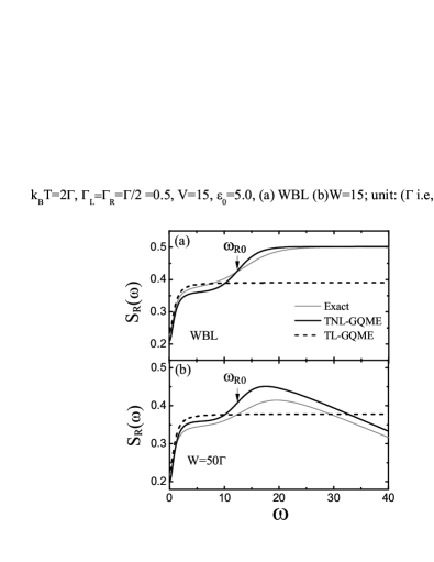
Figure 1: Noise spectrum for right reservoir, evaluated with three methods: exact (solid gray line), TNL-GQME (solid black line) and TL-GQME (dashed line) treatments for (a) WBL and (b) Finite band width of $W=50\Gamma$. The other parameters are (in arbitrary unit $\Gamma$): $\epsilon=5$, $\Gamma_{L}=\Gamma_{R}=0.5$, $k_{B}T=2$, and $eV=15$.

IV.2 Interacting single dot

The Coulomb interaction case is exemplified with

$$H=\epsilon_{\uparrow}\hat{n}_{\uparrow}+\epsilon_{\downarrow}\hat{n}_{\downarrow}+U\hat{n}_{\uparrow}\hat{n}_{\downarrow},$$ (30)

where $\hat{n}_{\mu}=d^{\dagger}_{\mu}d_{\mu}$. The annihilation operators are $d_{\uparrow}=|0\rangle\langle\uparrow\!\!|+|\!\!\downarrow\rangle\langle\uparrow\downarrow\!\!|$ and $d_{\downarrow}=|0\rangle\langle\downarrow\!\!|-|\!\!\uparrow\rangle\langle\uparrow\downarrow\!\!|$, with $|0\rangle$, $|\!\!\uparrow\rangle$, $|\!\!\downarrow\rangle$, and $|\!\!\uparrow\downarrow\rangle$ denoting the empty, two single–occupation spin states, and the double–occupation spin–pair state, respectively, in the Fock space. To have the Coulomb interaction effect more transparent, we set the dot level spin–degenerate, $\epsilon_{\uparrow}=\epsilon_{\downarrow}=\epsilon$, and focus on the transport in strong Coulomb blockade regime, $\epsilon+U>\mu_{\rm L}>\epsilon>\mu_{\rm R}$, where the stationary transport current is $\bar{I}=2\Gamma_{L}\Gamma_{R}/(2\Gamma_{L}+\Gamma_{R})$.

For the purpose of comparison later, we present here the results of TL–GQME based (Markovian) shot noise spectrum (denoting $\Gamma_{\rm eff}\equiv 2\Gamma_{\rm L}+\Gamma_{\rm R}$):Luo et al. (2007)

$$\begin{split}F^{\rm M}_{\alpha}(\omega)=\frac{4\Gamma_{\rm L}^{2}+\Gamma_{\rm R}^{2}+\omega^{2}}{\Gamma_{\rm eff}^{2}+\omega^{2}},\ \ \ F^{\rm M}_{c}(\omega)=\frac{2\omega^{2}}{\Gamma_{\rm eff}^{2}+\omega^{2}},\end{split}$$ (31)

which assume Poissonian, $F^{\rm M}_{\rm L}=F^{\rm M}_{\rm R}=1$ and $F^{\rm M}_{c}=2$, as $\omega\rightarrow\infty$. We will see soon that the TNL–GQME treatment will lead to very different behaviors, due to the increasing non-Markovian effect with increasing the detection frequency.

Figure 2: Noise spectrum of transport current [in $F(\omega)\equiv S(\omega)/(2\bar{I})$] through an interacting quantum dot, decomposed to (a) left junction current, (b) right junction current, and (c) charge-number fluctuation components, respectively. Parameters (in arbitrary unit $\Gamma$) are $U=25$, $k_{B}T=0.5$, and $\epsilon=2$, with different values of bandwidth $W$. The other parameters are the same as in Fig. 2.

Figure 2 depicts the noise spectrum of transport current, with different bandwidths that crossover the fixed Coulomb interaction parameter $U=25\,\Gamma$ to visualize the interplay between them. The non-Markovian quasi–step feature is displayed by a number of quasi–step jumps around the resonant frequencies of

$$\omega_{\alpha 0}=|\mu_{\alpha}-\epsilon|{\rm\ \ and\ \ }\omega_{\alpha 1}=\epsilon+U-\mu_{\alpha},$$ (32)

with $\alpha=$ L and R. Specifically, these resonance frequencies (in unit of $\Gamma$) are $\omega_{{\rm L}0}=5.5$, $\omega_{{\rm R}0}=9.5$, $\omega_{{\rm L}1}=19.5$, and $\omega_{{\rm R}1}=34.5$, for the parameters used in Fig. 2. This characteristic feature can be used to extract the information of the discrete energy level of the dot as well as the magnitude of the Coulomb interaction. The finite-frequency-support resulted from finite bandwidth is also apparent in interacting dots systems.

To highlight the quasi–steps resonant tunneling characteristics, we consider the WBL, with the aid of its approximated analytical results as follows. Let us start with the region of $\omega>\omega_{\alpha 0}$:

$$F_{\alpha}(\omega) =\left\{\begin{array}[]{ll}\frac{1}{2}(1+\gamma_{\alpha})\,;&\qquad\quad\ \omega_{\alpha 0}<\omega<\omega_{\alpha 1}\\ \frac{1}{2}+\gamma_{\alpha}\,;&\qquad\quad\ \omega>\omega_{\alpha 1}\end{array}\right.,$$ (33c)

$$F_{c}(\omega) =\left\{\begin{array}[]{ll}1+\frac{1}{2}(\gamma_{\rm L}+\gamma_{\rm R})\,;&\ \omega_{\rm R0}<\omega<\omega_{\rm L1}\\ 1+\gamma_{\rm L}+\frac{1}{2}\gamma_{\rm R}\,;&\ \omega_{\rm L1}<\omega<\omega_{\rm R1}\\ \frac{1}{2}(3+2\gamma_{\rm L}+\gamma_{\rm R})\,;&\ \omega>\omega_{\rm R1}\end{array}\right..$$ (33g)

Apparently, the noises depending on $\gamma_{\rm L}\equiv\Gamma_{\rm L}/\Gamma_{\rm R}\equiv 1/\gamma_{\rm R}$ can still be either super– or sub–Poissonian. Consider for example Eq. (33c), where the two regions are actually $\mu_{\rm L}>\epsilon,\epsilon+U>\mu_{\rm R}$ and $\epsilon+U>\mu_{\rm L}>\epsilon>\mu_{\rm R}$, representing the weak and the strong Coulomb interaction cases, respectively. Evidently the resonant quasi–step characteristics of noise spectrum are enhanced by Coulomb interaction [cf. Fig. 2 or Eq. (33), with $\omega>\omega_{\alpha 1}$].

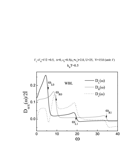
Figure 3: The dispersion function contribution to the noise spectrum through an interacting quantum dot, decomposed to left junction current (solid in black), right junction current (solid in gray), and charge–number fluctuation (dotted in black) components, respectively, with WBL. The parameters are the same as in Fig. 2.

Consider the low–frequency region ($\omega<\omega_{\alpha 0}$), where the noise spectrum can be analyzed via

$$F_{\alpha/c}(\omega)=F^{\rm M}_{\alpha/c}(\omega)-D_{\alpha/c}(\omega)/(2\bar{I}).$$ (34)

The first term is just the Markovian result Eq. (31). The second term accounts for the renormalization effect and can be evaluated in the WBL as

$$\begin{split}D_{L}(\omega)&=\frac{8\Pi_{\rm L}\Gamma_{\rm L}}{\big{(}\Gamma_{\rm eff}^{2}+\omega^{2}\big{)}\omega}\,,\ \ D_{R}(\omega)=\frac{2\Pi^{\prime}_{\rm R}\Gamma_{\rm R}}{\big{(}\Gamma_{\rm eff}^{2}+\omega^{2}\big{)}\omega}\,,\\ D_{c}(\omega)&=\frac{2(\Phi_{\rm L}+\Phi_{\rm R})[\Gamma_{\rm eff}(\Phi_{\rm L}+\Phi_{\rm R})-\Gamma_{\rm R}\omega]}{\Gamma_{\rm eff}^{2}+\omega^{2}},\end{split}$$ (35)

where $\Pi^{\prime}_{\rm R}=\Pi_{\rm R}+\Phi_{\rm R}\big{[}(1+\Gamma_{\rm L}/\Gamma_{\rm eff})\omega^{2}-6\Gamma^{2}_{\rm L}\big{]}$, and $\Pi_{\alpha}=\Phi_{\alpha}[\omega(\Phi_{\rm L}+\Phi_{\rm R})+2\Gamma^{2}_{\alpha^{\prime}}+\omega^{2}\Gamma_{\alpha^{\prime}}/\Gamma_{\rm eff}]+2\Gamma_{\rm L}\Gamma_{\rm R}(\Phi_{\rm L}-\Phi_{\rm R})$, with $\alpha^{\prime}\neq\alpha$. These non-Markovian contributions are related to the dispersion function, through [cf. Eq. (28)]

$$\Lambda^{(\pm)}_{\alpha}(\epsilon-\omega)-\Lambda^{(\pm)}_{\alpha}(\epsilon+\omega)\approx\phi_{\alpha}(\epsilon-\omega)-\phi_{\alpha}(\epsilon+\omega)\equiv\Phi_{\alpha}(\omega;\epsilon).$$

The renormalization is important especially in the low frequency regime, as shown in Fig. 3. Note that $D_{c}(0)=0$ but $D_{\alpha}(0)\neq 0$ at zero frequency. However, the renormalization effect on the central-dots charge fluctuation extends wider frequency range than that on the lead current fluctuation.

V Concluding remarks

In summary, we have presented the TNL-GQME and exploited it in analyzing the frequency dependence of shot noise spectrum. The theory itself is the extension of the conventional TNL-QME Yan and Xu (2005) to quantum measurement problems, via the standard particle counting $\chi$-field method.Levitov and Lesovik (1993); Levitov et al. (1996); Bagrets and Nazarov (2003) By comparing with the exact results on non-interacting dots, we numerically demonstrated that the TNL-GQME is more appropriate than its TL-counterpart. This observation clearly indicates that the shot noise spectrum of transport current is generally non-Markovian, even in the WBL of electron reservoirs leads.