Formation of water and methanol in star forming molecular clouds

Abstract

Aims. We study the formation of water and methanol in the dense cloud conditions to find the dependence of its production rate on the binding energies, reaction mechanisms, temperatures, and grain site number. We wish to find the effective grain surface area available for chemical reaction and the effective recombination timescales as functions of grain and gas parameters.

Methods. We used a Monte Carlo simulation to follow the chemical processes occurring on the grain surface. We carried out the simulations on the Olivine grains of different sizes, temperatures, gas phase abundances and different reaction mechanisms. We consider H, O, and CO as the accreting species from the gas phase and allow ten chemical reactions among them on the grains.

Results. We find that the formation rate of various molecules is strongly dependent on the binding energies. When the binding energies are high, it is very difficult to produce significant amounts of the molecular species. Instead, the grain is found to be full of atomic species. The production rates are found to depend on the number density in the gas phase. When the density is high, the production of various molecules on the grains is small as grain sites are quickly filled up by atomic species. If both the Eley-Rideal and Langmuir-Hinselwood mechanisms are considered, then the production rates are at this maximum and the grains are filled up relatively faster. Thus, if allowed, the Eley-Rideal mechanism can also play a major role and more so when the grain is full of immobile species. We show that the concept of the effective grain surface area, which we introduced in our earlier work, plays a significant role in grain chemistry.

Conclusions. We compute the abundance of water and methanol and show that the results strongly depend on the density and composition in the gas phase, as well as various grain parameters. In the rate equation, it is generally assumed that the recombination efficiencies are independent of the grain parameters, and the surface coverage. Presently, our computed parameter $\alpha$ for each product is found to depend on the accretion rate, the grain parameters and the surface coverage of the grain. We compare our results obtained from the rate equation and the one from the effective rate equation, which includes $\alpha$. A comparison of our results with the observed abundance shows very good agreement.

1 Introduction

Formation of complex organic molecules in the interstellar medium (ISM) is an active subject of research. Out of a host of organic and inorganic molecules that have been observed, water and methanol are most certainly two very important organic species found both in the gas and solid phases of ISM. The abundance of these species in the various regions of ISM is also different. It was thought for a long time that the water is one of the possible reservoirs of elemental oxygen in the gas phase, but recent Submillimeter Wave Astronomy Satellite (SWAS) observation found surprisingly a low abundance of water. Snell et al. (2000) find that the abundance of water relative to H₂ in Orion and M17 cloud is between $10^{-10}$ to $8\times 10^{-10}$. The water abundance in the hot cores range from $10^{-6}$ to $10^{-4}$ (van Dishoeck & Helmich 1996, Helmich et al. 1996; Boogert & Ehrenfreund, 2004). The abundance of water on grains with respect to the total H column density is typically $10^{-4}$ and is the most abundant component (Tielens et al. 1991). Similarly, interstellar methanol has three types of abundance profile: flat profiles at CH₃OH/H₂ $\sim 10^{-9}$ for the coldest sources, profiles with a jump in its abundance from $\sim 10^{-9}$ to $\sim 10^{-7}$ for the warmer sources, and flat profiles at a $\sim$ few $10^{-8}$ for the hot cores (van der Tak et al. 2000). On the grain surface, the methanol abundance varies from $5\%$ to $30\%$ with respect to H₂O. In some sources, such as SgrA and Elias 16, the abundance is even less (Gibb at al., 2000). The observed abundance for methanol along the line of sight towards high mass and low-mass proto-stars is between $0.2-2\times 10^{-5}$ (Gibb et al. 2004; Pontoppidan et al. 2003, 2004). Much higher methanol abundances are found to be associated with the outflows in the regions of low mass star formation, L1157-MM and NGC1333-IRAS2 $2\times 10^{-5}$ and $2\times 10^{-6}$ (Bachiller & Perez Gutierrez, 1997; Bachiller et al. 1998). In other words, either on the grain surfaces or in the hotter region, abundances of theses species are high. This correlation suggests that these species perhaps originate from grains and their productions in the gas phase are inadequate. Therefore, the understanding of the formation of water and methanol on grain surfaces is of primary importance.

The grain surface reactions were first introduced to explain the formation of molecular hydrogen (Hollenbach & Salpeter, 1970). Since then it has been used very extensively by several authors (Watson & Salpeter 1972ab; Allen & Robinson 1975, 1976, 1977; Tielens & Hagen 1982; Hasegawa & Herbst 1992; Charnley 2001; Stantcheva et al. 2002, Green et al. 2001; Biham et al. 2001; Stantcheva et al. 2002). These studies mainly belong to two different categories, the deterministic approach and the stochastic approach. In the deterministic approach, one can completely determine the time evolution of the system once the initial conditions are known. The rate equation method belongs to this category. This method is very extensively used by several authors to study the grain surface chemistry (Hasegawa & Herbst 1992; Roberts et al. 2002; Acharyya et al. 2005). However, this method is only applicable when there are large numbers of reactants on the grain surface. Given that the interstellar medium is very dilute, very often this criteria is not fulfilled and this method cannot be applied. But this method is computationally faster and can very easily be coupled with the gas phase reactions. In the stochastic approach, fluctuations in the surface abundance due to the statistical nature of the grain is preserved. The Monte Carlo method and the Master equation methods belong to this category. Both these methods are used by several authors (Charnley 2001; Stantcheva et al. 2002, Green et al. 2001; Biham et al. 2001; Stantcheva et al. 2002 ). Its major disadvantage is that it takes enormous computational time. Coupling of the Monte Carlo method (for grain surface reactions) and rate equation method (for gas phase reactions) is extremely difficult. Although the Master equation method can be coupled with the rate equations, but it is disadvantageous because one has to solve a large number (ideally infinite) of reactions.

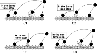
Figure 1: Cartoon diagram to show the different reaction schemes (C1-C4) that are considered in our calculation. Black and shaded circles are representatives of reactive species and the clear circles are for nonreactive species. A circle around two such species indicates that the new species is created due to Eley-Rideal scheme.

Recently, Chang et al. (2005) have argued that the stochastic methods used so far can also lead to error because the rate of reaction is determined by the rate of hopping (or tunneling) of a hydrogen atom from one site to the nearest neighboring site multiplied by the probability of finding a reactant partner in this site. This is also an average treatment since, on any given grain, the reactant partner is unlikely to lie in the nearest-neighboring site. They used a continuous random work technique to study the formation of molecular hydrogen. Chakrabarti et al. (2006ab) used a similar method that keeps track of each individual reactant and their movements and calculated the effective grain surface area involved in the formation of molecular hydrogen in the interstellar clouds. Chakrabarti et al. (2006, hereafter referred as Paper-I) illustrated that the formation rate per unit grain site itself strongly depends on the nature and size (i.e., no. of sites) of the grains for a given gas phase condition (abundance, temperature, etc.). In Paper-I, this was demonstrated only for H forming H₂ molecules. In the present paper, we carry out a similar analysis where we consider the accretion of H, O, and CO onto the grain surface and show that the formation rates of water and methanol are indeed dependent on the intrinsic and extrinsic parameters of the system. The plan of this paper is the following. In the next section, we discuss various mechanisms of reactions on the surface. In Section 3, we discuss the procedure of our computation. In Section 4, we describe various models used for our simulations. In Section 5, we present our results. Finally, in Section 6, we draw our conclusions.

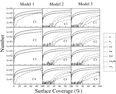
Figure 2: Evolutions of the number of a few selected species on a grain having $10^{4}$ sites are shown with respect to the surface coverage of a mono-layer (along X-axis), for various sets of binding energies (Models 1-3) and for different mechanisms (C1-C4). These simulations were carried out for high abundances of the accreting species (Table 1). Different styles of the curves are marked with the species names on the right. Note that methanol and CO₂ are absent in the Model 1 simulation where the binding energy was very high.

2 Mechanisms of reactions on grain surfaces

A thorough understanding of the surface reaction mechanisms requires knowing of the basic physical processes involved when the gas phase atoms and molecules interact with the grains. The first step is accretion, i.e., landing various species onto a grain surface. In our case, only H, O, and CO are taken as the accreting species onto the grain surface. In the next step, the accreted species will react to form various new species. There are two reaction schemes, the Langmuir-Hinselwood (LH) mechanism and the Eley-Rideal (ER) mechanism. In the LH scheme, the gas phase species accretes onto a grain and becomes equilibrated with the surface before it reacts with another atom or molecule, and in the ER reaction scheme, the incident gas phase species collides directly with an adsorbed species on the surface and reacts with that species. In such a mechanism, the reactant generally does not become trapped at the surface and it is unlikely to be sensitive to the surface temperature (Farebrother et al. 2000). In our study, we considered that the reaction on a surface can occur through both LH and ER mechanisms. However, we assume that the molecules are trapped after reaction due to their high binding energy.

The binding energy of the incoming species strongly depends on the species itself and on the way the interaction proceeds. The incoming species might get trapped in a shallow potential well in a physisorbed site. The interaction is mainly due to mutually induced dipole moments or it might also form a strong covalent bond. Recent studies have found evidence of both physisorption and chemisorption processes taking place on a grain surface. However, for the chemisorption, a higher kinetic energy is involved, so this type of interaction is not relevant except in very special astrophysical conditions. We have considered only weakly bound species, i.e., physisorbed atoms and molecules. The typical energy for physisorption is around $0.1$ eV or $\sim\ 1000$ K. If $E_{d}$ denotes the binding energy for physical adsorption and $E_{b}$ the potential energy barrier, then $E_{d}$ must be greater than $E_{b}$ for the species to diffuse from one site to the other.

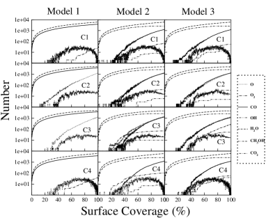
Figure 3: Same as in Fig. 2, but the low abundances of the accreting species have been chosen.

For a chemical reaction to occur, an accreted species has to scan the grain surface in search of a reaction partner. There are two physical processes that can provide the mobility for the accreted gas phase species, the thermal hopping and tunneling. As mentioned earlier, Hollenbach & Salpeter first introduced the grain surface chemistry to explain the high abundance of molecular hydrogen. They assumed that, within the grains, the hydrogen atoms move from site to site by a quantum mechanical tunneling process. But from the recent experimental results of molecular hydrogen formation, it was found that the mobility of hydrogen on grains is primarily due to the thermal hopping (Pirrenello 1997ab, 1999). The tunneling time very dependent on the mass of the particle and the barrier thickness, a unknown parameter. Therefore, it is not widely used in the astrophysical models. The classical papers like Tielens & Hagen (1982) and Hasegawa & Herbst (1992) considered the tunneling for hydrogen and thermal hopping for other simple atoms and molecules. We considered both tunneling and thermal hopping for the hydrogen atoms and only thermal hopping for others.

If we consider the time scale for hopping and tunneling for the hydrogen atom and hopping for other species, we observe that the mobility of hydrogen atom is much greater than for the other reactive species. The hopping and tunneling time for hydrogen is $\sim 7.4\times 10^{-09}$ and $2.0\times 10^{-11}$s, and the hopping times for atomic species like O and CO are $\sim 2.4\times 10^{-2}$s and $\sim 5589$s , respectively. Therefore, the hydrogenation reactions are the dominant reactions on grains.

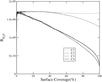
Figure 4: Rate of production of H₂O is shown against the surface coverage for the four different schemes mentioned in the text. The production is high when the Eley-Rideal mechanism is taken into account, while the production is lower when the reaction takes place at the next time step. The rate is computed using (a) the total production and total time taken at a given instant, (b) the change in the number of H₂O for a fixed change in parcentage of the surface coverage.

2.1 Accretion rate

Accretion is the process by which grain receives matter. We define the accretion rate [$r_{acc}(i)$] for a given neutral species $i$ in the units of s^-1 , as

$$r_{acc}(i)=s_{i}\sigma v_{i}n_{gas}(i),$$ (1)

where $s_{i}$ is the sticking coefficient (taken as $1$ for all the three species), $v_{i}$ the velocity (cm s^-1 ), $n_{gas}(i)$ is the gas phase number density (cm^-3) of the $i$-th species, and $\sigma$ the grain cross-section (cm²). In this paper, we carry out our calculation usually for two different sets of gas phase number densities, excepts towards the end where we compared results from several number densities. Thus, we have two sets of accretion rates. Number densities are taken from Stantcheva et al. (2002). These are listed in Table 1.

Table 1: Gas-phase abundances used

Species	high ($cm^{-3}$)	low ($cm^{-3}$)
H	1.10	1.15
O	7.0	0.09
CO	7.5	0.075

2.2 Diffusion rate coefficients and binding energies

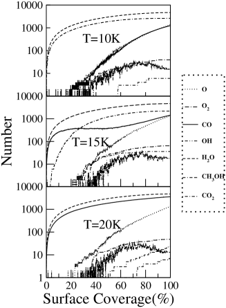
Figure 5: Rate of production of a few selected species as a function of surface coverage at different temperatures shown for a grain having $10^{4}$ sites for Model 2 and C2 scheme. These simulations were carried out for low abundances of the accreting species.

The diffusion rate coefficients ($k$) are the sums of the rates $t^{-1}_{diff}$ ($s^{-1}$) the reactive species need to traverse an entire grain ($t_{diff}$ is the diffusion time). In the present paper, we are interested in showing the size dependence of the recombination process. Thus, we choose a grain to contain $10^{4}$ to $10^{5}$ sites. The rate coefficient is usually multiplied by a factor $\kappa$ that accounts for any non zero activation barrier (Hasegawa et al. 1992).

The rates depend strongly on $E_{b}$, the barrier energy. We considered three different sets of barrier energies. In the first set, we used the binding energies that come from the earlier works (Allen & Robinson, 1977; Tielens & Allamandola, 1987; Hasegawa & Herbst, 1993). We show them in Table 3. In this set, we considered that the hydrogen diffusion is caused by thermal hopping. Thus we ignore tunneling. In the second set, we used the same set of binding energies except for hydrogen diffusion procedure. Instead of hydrogen diffusion, we considered tunneling. Since the hydrogen diffuses much faster on grains than any other species, hydrogenation reaction is the dominant reaction on grains. This is why we did done our simulation for both thermal hopping and tunneling of hydrogen. The third set is based on recent findings of Pirronello et al. (1997, 1999) as interpreted by Katz et al. (1999), which show that atomic hydrogen moves much more slowly than what is used in various simulations. Therefore, in this set we used hydrogen hopping rates from Katz et al. (1999) and barrier energies for other species are increased proportionately (Table 2). This means that the ratio between the barrier energies of these two tables for different species are exactly the same as for H (i.e., $2.87$ for $E_{b}$ and $1.066$ for $E_{d}$). The ratio between the desorption energies of Table 2 and 3 was also kept fixed for simplicity. We chose $E_{b}=0.3E_{d}$ in Table 3 for all species except for H.

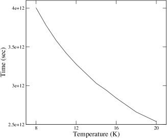
Figure 6: Plot of the time to build a mono-layer as a function of temperature for a grain having $10^{4}$ sites and for Model 2 by considering the C2 scheme. These simulations were carried out for low abundances of the accreting species.

Using these three sets we have constructed three models. The results are shown according to the increasing diffusion rate of hydrogen. Thus in Model 1, we used the slowest diffusion rate of hydrogen and hence the binding energy of Table 2. In Model 2, we used the binding energy from Table 3 (below). Finally in Model 3, the hydrogen tunneling is considered and the binding energy is taken from Table 3 for other species.

Table 2: Energy barriers against diffusion and desorption in K for the olivine grain (from experiment)

Species	$E_{b}$	$E_{d}$
H	287	373
O	689	853
OH	1085	1343
$\mathrm{H_{2}}$	387	479
$\mathrm{O_{2}}$	1042	1290
$\mathrm{H_{2}O}$	1601	1982
CO	1042	1290
HCO	1300	1609
$\mathrm{H_{2}CO}$	1515	1876
$\mathrm{CH_{3}O}$	1868	2313
$\mathrm{CH_{3}OH}$	1774	2195
$\mathrm{CO_{2}}$	2153	2664

Table 3: Energy barriers against diffusion and desorption in K for the olivine grain (See text for references.)

Species	$E_{b}$	$E_{d}$
H	100	350
O	240	800
OH	378	1260
$\mathrm{H_{2}}$	135	450
$\mathrm{O_{2}}$	363	1210
$\mathrm{H_{2}O}$	558	1860
CO	363	1210
HCO	453	1510
$\mathrm{H_{2}CO}$	528	1760
$\mathrm{CH_{3}O}$	651	2170
$\mathrm{CH_{3}OH}$	618	2060
CO2	750	2500

3 Simulation procedure

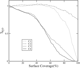
Figure 7: Variations in $\gamma_{H_{2}O}(t)$ with surface coverage for different reaction schemes for Model 2. Note that when the Eley-Rideal scheme is included (C1 and C4) the production efficiency increases rapidly as the grain is filled up.

We used a Monte-Carlo simulation method of studing the chemical evolution on grains in the presence of H, O, and CO as accreting species. For the sake of simplicity we assume that a grain is square shaped having $S$ number of sites. For concreteness we chose olivine grains having the surface density of sites $s=1.5\times 10^{15}$ cm^-2 (Hasegawa et al. 1992). We assumed further that each site has four nearest neighbors, as in an fcc[100] plane. To mimic the spherical grain structure, we assumed a periodic boundary condition, i.e., a species leaving the boundary site of a grain on one side enters back into the grain from the opposite side.

In our method of simulation, self-crossing paths of randomly walking atom are automatically included (some times called the back-diffusion in the literature, e.g., Chang et al. 2005). The minimum time step of our simulation is assumed to be the time taken for hopping or tunneling (whichever is smaller) of a H atom from site to site. If $r_{acc}$ is the astrophysically relevant accretion rate under consideration, the $i$-th species will have to be dropped after every $1/r_{acc}$ seconds. The location of the accreting $i$-th species is obtained from a pair of random numbers ($R_{x},R_{y}$), themselves obtained by a random number generator. This pair would place the incoming species at ($j$, $k$)-th site of the grain, where $j$ and $k$ are the nearest integers obtained using Int function: $j=int(R_{x}*n+0.5)$ and $k=int(R_{y}*n+0.5)$. Here, $n=\sqrt{S}$, being the number of sites on a square. Now during the hopping or tunneling process, when one species enters the site that is already occupied by another reactant surface species, it will form a molecule if activation barrier energy permits. Thermal evaporation of a species is also handled by random numbers. After each hopping and tunneling time, we generate a random number ($R_{t}$) for $i$-th species, if $R_{t}$ is less than $W_{i}/a_{h_{i}}$ or $W_{i}/a_{t_{i}}$. Then we allow that species to evaporate. Here, $W_{i}$ is the desorption rate and $a_{h_{i}}$ and $a_{t_{i}}$ are the rates of hopping and tunneling of the $i$-th species, respectively. We carry out our simulation up to the time within which one monolayer is produced. We wish to make a remark in passing that a totally different random number generator was also found to yield a similar result, so thus we believe that the results we present in this paper do not depend on a random number generator.

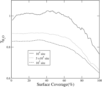
Figure 8: Variation in $\gamma_{H_{2}O}(t)$ with the surface coverage for different grain sizes. Here, the binding energies of Model 2 are used. Note that $\gamma_{H_{2}O}(t)$ is decreased with increasing grain size since the probability of capturing an incoming species increases with the grain size. Here C2 scheme has been chosen.

Keeping in mind that there are two types of reaction schemes, the landing of a gas phase atom or molecule can have one of these two distinct fates. It can land either on a vacant site or on an occupied site. When the landing is on a vacant site, the follow-up computation is straightforward. The species will simply start scanning the surface for a reactive partner. When it lands on an occupied site, however, there could be two possibilities, (i) The incoming species can land directly on a reactive species but it may or may not combine with it. If not, it will look for an alternate site for itself. (ii) The incoming species can land directly on a nonreactive species and look for an alternate site. However, looking for an alternate site itself could be achieved in two ways: in the same time step (which is more likely) or in the next time step. Thus we can have a total of four different models in the simulation. These are illustrated in a cartoon diagram C1-C4 in Fig. 1. In C1, both the LH and ER schemes are considered, i.e., the incoming atom/molecule is allowed to land on both the unoccupied and occupied sites. With the reactive species, it combines to form a new species (marked with a common circle). It skips the nonreactive species and looks for a new site in the same time step. C4 is otherwise the same as C1, but the incoming species looks for a new site at the next time step after it lands on a nonreactive species. In C2, the incoming species lands on a reactive species, but does not combine and insteads finds a new site at the same time step (LH mechanism). C3 is the same as C2, but we allow the landing at a new time step.

Table 4: Surface Reactions in the H, O, and CO model

Number	Reactions	Ea(K)
1	H+H $\rightarrow$ H2
2	H+O $\rightarrow$ OH
3	H+OH $\rightarrow$ H2O
4	H+CO $\rightarrow$ HCO	2000
5	H+HCO $\rightarrow$ H2CO
6	H+H2CO $\rightarrow$ H3CO	2000
7	H+H3CO $\rightarrow$ CH3OH
8	O+O $\rightarrow$ O2
9	O+CO $\rightarrow$ CO2	1000
10	O+HCO $\rightarrow$ CO2+H

4 Model simulations

We consider that only three species, namely, H, O, and CO are accreting in the grain phase, and we assume that ten types of reactions can go on among these constituents. These are listed in Table 4. Let us consider a reaction of the type,

$$a+b\longrightarrow c.$$ (2)

The rate of variation of any molecular species $c$ with time is usually taken as (see, Paper-I and references therein)

$$\frac{dn_{c}}{dt}=r_{ab}n_{a}n_{b}/S$$ (3)

where, $n_{a}$, $n_{b}$, and $n_{c}$ are the concentrations of the species $a$, $b$,and $c$ on a grain. Here, $r_{ab}$ is the rate of formation of $c$ out of $a$ and $b$, and $S$ is the number of sites on the grain. The rate $r_{ab}/S$ is approximately the inverse of the time required for an atom to visit nearly all the adsorption sites on the grain surface. This is because, in two dimensions, the number of distinct sites visited by a random walker is linearly proportional to the number of steps, up to a logarithmic correction. But in a realistic situation, this is not the case for two reasons (Paper-I). The first is that the number of hoppings to find a reactant partner depends on the number of atoms or molecules already occupying the grain. When the grain is almost empty, a species has to hop several times, and when the grain is full, it requires less of hops, so the ‘size’ of a grain is relative as far as the hoping element is concerned. The second reason is the blocking effect. This phenomenon is seen very often on a grain having a mono-layer. On a grain surface, the interaction of species is generally considered to be with those located in the four nearest neighboring sites. A possible scenario would be that a reactive species is blocked in all the four directions due to the presence of various species with which no reaction is allowed. For instance, if a CO molecule lands on a site surrounded by H₂O molecules, it cannot react and will wait there itself for its desorption unless the blocked species themselves desorb and free the sites for the landed species to move around. The effect becomes more severe as the grains start getting filled up. In the latter case, the blocking effect will weaken when the blocked element overcomes the energy barrier. As the surface is populated, these types of effects become more and more prominent. To understand the influence of these processes on the recombination, we define two parameters, namely, $\gamma$ and $\alpha$ as given below.

Figure 9: Variation in $\alpha_{H_{2}O}(t)$ with surface coverage for different reaction schemes as in Fig. 7. The formation rate of the new species goes down (i.e., $\alpha_{H_{2}O}(t)$ goes up) for C2 and C3 since the species is created in the next time step.

If $t_{c}$ is the “average time” required to form a species $c$ after the species $a$ and $b$ are simultaneously present in our simulation, then $\frac{dn_{c}}{dt}\sim n_{a}n_{b}/t_{c}$, where $t_{c}=r_{ab}/S$. The rate with which the species $c$ is formed is $1/t_{c}$. Because of the two effects mentioned above, the actual rate may be assumed to be $r_{ab}/S^{\gamma}_{c}$ instead of $r_{ab}/S$. From the above equation,

$$\gamma_{c}=\frac{log[r_{ab}t_{c}]}{logS}.$$ (4)

As an example, let us consider the calculation of $\gamma_{c}$ for H₂O. Since H has a very small desorption time scale compared to the other species, it will desorb from the grain if it does not find a reaction partner within its desorption time scale. If H gets another OH to form H₂O, then we calculate $dt_{H_{2}O}$ by noting down the time required to form an H₂O after the accretion of an H. At the beginning of the simulation, most of the sites are empty and one H will have to more or less scan the whole of the grain to find its reactant partner. and hence will take longer time to form a molecule. On the contrary, when most of the sites are filled with the different species, it will take less time to form a molecule and $\gamma_{c}$ should decrease. When a molecule is formed due to direct hitting, i.e., through the ER mechanism, $\gamma_{c}$ is clearly zero, since production rate is independent of the population of the species on the grain. Thus, if ER mechanism is included, $\gamma_{c}$ tends to become negligible as the grain is populated.

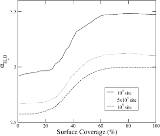
Figure 10: Same as in Fig. 8 except that $\alpha_{H_{2}O}(t)$ has been plotted. As the grain size gets smaller, $\alpha_{H_{2}O}$ increases, i.e., the recombination efficiency decreases. See text for details.

While $\gamma$ is derived from the time interval between the release of the reactants and the actual reaction to take place, another quantity, namely $\alpha$ may be defined to consider the cumulative effects and thus depends on the total time taken since the start of the accretion onto the grain. Because of the two competing processes mentioned at the beginning of this section, there will be a net change in the rate equation itself with time, since $\alpha$ itself will be time dependent. To quantify this, we replace $r_{ab}/S$ in Eq. 3 by $r_{ab}/S^{\alpha(t)}$. Thus, the Eq. 3, which is rewritten as

$$log{\frac{dn_{c}}{dt}}=log[r_{ab}n_{a}n_{b}/S^{\alpha_{c}(t)}],$$ (5)

can be used to obtain $\alpha_{c}(t)$ as

$$\alpha_{c}(t)=log[\frac{(r_{ab}n_{a}n_{b})}{\frac{dn_{c}}{dt}}]/log(S).$$ (6)

Note that, for reactions between the similar species, their will have to be a factor of $1/2$ inside the logarithmic expression (see, Paper-I for H₂ formation) to reduce the possibility of double counting. As the surface is populated by a number of reactant species, the recombination time scale would vary with time and thus $\alpha_{c}(t)$ will also vary. As mentioned before, the time $t$ used in computing $\alpha$ is the total time taken since the grain starts populating. On the other hand, $\gamma$ is an average quantity that is computed instantaneously.

We run the simulations to show that $\alpha(t)$ and $\gamma$ are not necessarily unity. This means that the surface chemistry is not just a matter of random hopping, since the degree of randomness is seriously modified with the population and the abundance of species on the grain surface. The Monte-Carlo simulation reflects a more realistic computation, but it is very time-consuming. In a large-scale computation, it is impractical to do such a simulation. Indeed, we also show that only when $\alpha$ as given above is used in the effective rate equation (where every $S$ is replaced by $S^{\alpha}_{i}$, where $\alpha_{i}$ is different for different species), then the abundances of each species obtained from such an equation agree with the results of the Monte-Carlo simulation. Thus, one may as well solve the effective rate equation using $\alpha$ obtained from our calculations. We have made a table for $\alpha$ (Table 7 , below) for future. However, discussions of its approximate value, shape, and dependence is beyond the scope of this paper and will be discussed elsewhere.

In what follows, we ran twelve different cases. For each set of binding energies, all the four C1, C2, C3, and C4 cases are considered. Due to the complexity of the system, we restricted ourselves only up to the formation of a mono-layer on the grain surface.

5 Results

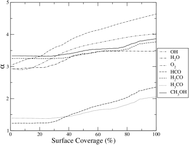
Figure 11: Variation in $\alpha$ with the surface coverage for various molecular species that form on the grain surface. All of them deviate from unity. This case is for Model 2 with the C2 scheme.

We first carried out the simulation for a grain having $10^{4}$ sites. We considered two different sets of gas-phase abundances in our study, one with a high density and the other with low density. For each set of gas-phase abundances, we consider three sets of binding energies and for each set of binding energies we have four cases, C1, C2, C3, and C4 as described in Section 3. Thus for each set of gas-phase abundance, we essentially have twelve different cases.

5.1 Grain surface abundances

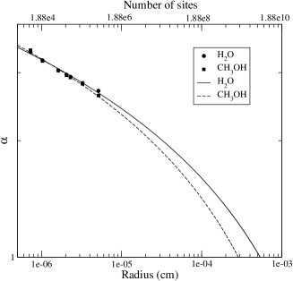
Figure 12: Variations in $\alpha$ for water and methanol (averaged over the surface coverage) as functions of the grain radius and no. of sites on the grain. The filled circles are for $H_{2}O$ and the filled boxes are for methanol. The corresponding fitted curves are also shown. They are extrapolated to larger grain sizes.

In Fig. 2, we show the results for the high gas-phase abundances. In the first column, the plots correspond to the binding energies of Model 1 as mentioned in the Table 2 are shown. The binding energies are high and consequently the diffusion rates are low. Let us first consider C1 and C2 cases. We note that, respectively, only $16\%$ and $11\%$ of the grain deposition is water. This low production of water is due to the slow diffusion rate and due to the absence of sufficient number of hydrogen atoms to react with the oxygen atom. In C1, the excess of production of water by four per cent is mainly due to ER mechanism. There is hardly any methanol produced due to slow diffusion rate and due to presence of an activation barrier energy. In C1, around $19\%$ of molecular oxygen is produced, but its absence in C2 suggests that it is produced due to the ER mechanism. Around $50\%$ of the grain surface abundance is CO. The time required to grow one mono layer for C1 and C2 is $1600$ years and $1300$ years, respectively. The grain is very quickly filled up by the accreted species. The results for the cases C3 and C4 differ only slightly in comparison to C2 and C1, respectively. Only a small increase in the molecular species and decrease in the atomic species is observed. The times required to grow a mono layer in C3 and C4 are around $13000$ years and $36000$ years, respectively. This longer timescale is due to the fact that in these cases atoms/molecules are not bound to accrete on the same time step. In the case of C4 we continue our simulation up to the time when all O and OH are converted to H₂O, hence the time taken is much longer.

The second and third columns show the plots corresponding to binding energies as mentioned in Table 3. In the second column, the hydrogen diffusion is due to the thermal hopping, whereas in the third column this is due to tunneling. These binding energies are low and the diffusion rates are consequently high. In all the four cases, the most dominant species are CO, O₂, and water. Water abundance is very similar, varying between $11\%$ and $19\%$. A very small amount of methanol has been produced. In all the cases, the production of a significant amount of molecular oxygen suggests that the ER mechanism may have an active role to play. The time required to grow a mono-layer is around $1500$ years. The third column also shows a similar trend of the results.

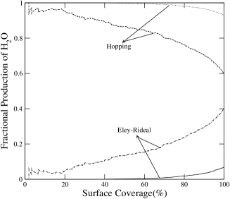
Figure 13: Variation in the fractional productions of H₂O through ER and LH schemes against the surface coverage of a mono-layer. For low surface coverage, H₂O production is dominated by the hopping process and when surface coverage is higher, the Eley-Rideal mechanism contributes in a major way towards the H₂O production. The uppermost and the lowermost curves are for the Model 2 energy and C1 scheme, with the low abundances of the accreting species. We compare the same for Model 1 energy with C1 method, with the high abundances for the accreting species (middle two curves).

In Fig. 3, we show the results for low gas-phase abundance. A significant amount of water is produced in all the cases, since the H/O and H/CO is relatively high. The presence of the atomic oxygen and carbon monoxide is also much lower, especially for Models 2 and 3. This is because, in the last cases the mobility of H being many orders of magnitude higher hydrogenation process is more efficient and that uses up O and CO to create water and methanol. This makes the production of methanol significant for Models 2 and 3 and insignificant for Model 1. Compared to the high abundance cases (Fig. 2), the accretion rate for low abundance is much lower, so the grain is not has full of atomic species as before. The time required to grow a mono-layer is around $0.1$Myr for both the cases. A similar trend is found for C3 and C4, but it takes around $1$Myr to fill up the grain. The second and third columns of Fig. 3 show a similar result. In all the cases, the most dominant species is water. The abundance of water varies between $46\%$ and $61\%$. The next dominant species is methanol with an abundance between $26\%$ and $33\%$. But only a trace amount of molecular oxygen is produced. Table 5 shows the percentage abundances for selected species, and Table 6 shows the time required to grow a mono-layer.

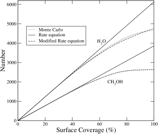
Figure 14: Comparisons of the number of H₂O and CH₃OH on a grain of $10^{4}$ sites as obtained by the rate equation method, the Monte-Carlo method, and the effective rate equation method. Here we chose the Model 2 energies and C2 with the low abundances case. The agreement between the Monte-Carlo result and the effective rate equation result is very good.

Figure 4(a-b) shows the rate $R_{H_{2}O}$ of production of H₂O for various mechanisms. This has been computed in two ways. Figure 4a shows the cumulative average rate where $R_{H_{2}O}=$H₂O$(t)/t$. We clearly see that, unless the production rate is very high (e.g. in case of C1), the cumulative rate generally falls off very rapidly with time. In the C1 scheme, the abundance of H₂O is higher because the formation of H₂O is dominated by direct hitting rather than hopping. In Fig. 4b, we plot $R_{H_{2}O}=\frac{dH_{2}O}{dt}$, where $d$H₂O is the production of H₂O in $dt$ time in which a fixed percentage $dp\%$ of the surface coverage is increased. Thus, in effect, it is the instantaneous rate. For simplicity, we choose $dp=10\%$ so as to get smooth curves. In the case of the LH scheme, i.e., for C2 and C3, as the surface starts to populate, the rejection of the incoming species become important and thus the rate of production decreases with the surface coverage.

5.2 Temperature dependence

Figure 5 shows the production of various species as a function of surface coverage at $10$ K, $15$ K and $20$ K. We carried out this computation only for Model 2 and taking low abundances of the accreting species. In all the three temperatures, the water is the most abundant species. But CH₃OH is only efficiently formed in $10$ K and $15$ K. At $20$ K, methanol production is significantly low because the desorption time scale of atomic hydrogen is much shorter and, at the same time, the activation barrier energy is much higher to produce methanol. It is instructive to study the time taken to fill up the grain. In Fig. 6 we plot the time required to build a mono-layer on a grain of $10^{4}$ sites as a function of the temperature of the grain. At higher temperatures, the time taken is lower because the grain is full of nonreactive CO (Fig. 6).

5.3 Variation in $\gamma$ and $\alpha$

In Fig. 7, the variation in ‘catalytic capacity’ for water, namely, $\gamma_{H_{2}O}(t)$ (Eq. 4) is shown as a function of the surface coverage. The figure shows that $\gamma_{H_{2}O}(t)$ gradually decreases with the surface coverage. This is because an increase in the surface coverage will decrease the number of vacant sites and will decrease the time for searching its reactant partner to recombine. The blocking effect also shows its effect by reducing $\gamma_{H_{2}O}$ very rapidly. The lower the value of $\gamma_{H_{2}O}$, the more efficient the recombination. This parameter is dependent on the number of sites on the grain. Figure 8 shows the change of $\gamma_{H_{2}O}$ with the number of grain sites. Naively, one would have expected that $\gamma_{H_{2}O}$ to remain unity always. In that case, $\gamma_{H_{2}O}$ would be independent of number of sites in the grain. However, we find that $\gamma_{H_{2}O}$ goes down with increase in $S$. From Eq. (4) we note that, when $S$ is increased from $10^{4}$ to $10^{5}$, the value of $\gamma_{H_{2}O}$ should go down by about $20\%$. This is roughly what is seen in the figure.

In Fig. 9, the variation in $\alpha_{H_{2}O}$ (Eq. 6) for water is shown as a function of time, which is represented here as the surface coverage. Here $10^{4}$ sites are chosen. This exponent deviates significantly from $1$. This deviation is mainly due to blocking the reacting species by the nonreactive species and the population of various species on the grain surface. This is particularly true for cases C2 and C3, since the ER mechanism was not assumed. For those with an ER mechanism (C1 and C4), the numbers actually go down, so the formation rate goes up. In Fig. 10, we plot the variation in $\alpha_{H_{2}0}$ as a function of surface coverage for a different number of sites on the grain. As the number of sites increases, $\alpha_{H_{2}O}$ is seen to decrease as in the case of $\gamma_{H_{2}O}$. We thus observe that the production rate of any species goes up for larger grains. To judge the implication of this in a cloud, we note that the dependence of the number density on the radius $r$ goes typically as $r^{-3.5}$ (Mathis et al. 1977), while the dependence of the production rate is $r^{n}$ with $n\sim 1$. Thus the production is still dominated by the smaller grains. However, smaller grains are lesser stable and could easily evaporate. This aspect clearly requires more thorough study.

In Fig. 11, we plot $\alpha$ for various species as a function of surface coverage when $10^{4}$ sites and the Model 2 with C2 mechanism were chosen. The most important observation from this is that $\alpha$ is not unity for any of these species. Second, up to about $30\%$ of the surface coverage $\alpha$ roughly remains constant, but after that all of them are going up monotonically as the surface gets filled up. Here the ER scheme is not used, and the formation rate goes down with coverage.

Since we generally see that $\alpha$ deviates from unity for smaller grains, it is pertinent to ask at, roughly what grain sizes $\alpha$ becomes unity. This would give us a region in which the classical rate equation would be valid. In Fig. 12, we show the variations in $\alpha$ for water and methanol are shown as functions of the grain radius and number of sites on the grain. The corresponding fitted curves are also shown. They are extrapolated to larger grain sizes. We note that, $\alpha\sim 1$ at around $r\sim 3-5\mu$m. Since the computational time to actually carry out the simulation at this size is prohibitively high, it could not be independently verified if this conclusion is rigorously valid. On the other hand, the number of grains at this size is expected to be negligible, and thus the exact knowledge of this limit may not be essential.

5.4 A comparison between LH and ER schemes

Figure 15: The ratio of methanol and water abundances on the grain surface plotted against the number density of the accreting gas. From the figure it is clear that as the number density goes up, methanol production goes down. The observed abundance of solid state methanol w.r.t. water is 5%-30%. From the figure it is to be noted that the region lies in the range $2.6\times 10^{4}$ to $8\times 10^{4}$. These simulation were carried out for Model 2 by considering the C2 method.

In Fig. 13, we plot the fractional production of H₂O for two different schemes at a given surface coverage to show the relative importance between the ER and LH schemes. Initially, when most of the sites are empty, the production of H₂O is mainly due to the hopping mechanism i.e., the LH scheme. As the grain starts to populate, the ER scheme starts to play an important role. In the figure, the uppermost and the lowermost curves are obtained using the low abundance set with C1 model. The other pair of curves is for a higher abundance set in the gas phase. Here the effect is more prominent. In general, the abundance of all the species is always a few $\%$ higher if the ER scheme is allowed.

5.5 Comparison of results with the effective rate equations

It may be instructive to check if the rate equations are modified with $r_{ab}/S$ replaced by $r_{ab}/S^{\alpha}$ everywhere, and they are solved by the usual method (Acharyya et al. 2005), then whether the results become comparable to those obtained from our Monte-Carlo method. In Fig. 14, we made a comparison of the abundances of two of the important species, namely, H₂O and CH₃OH in different methods. The results of our simulation clearly agree with those from the effective rate equation very well, but not with the original rate equation. This indicates that the $\alpha$s we introduced are very important and their effects are to be taken into account for accurately estimating of the species from the grain chemistry. Indeed, using the well-known MRN model of grain size, we find that water and methanol will be underproduced by $\sim 25\%$ and $\sim 33\%$, respectively, when the effective rate equations are used instead of the usual rate equation.

Since $\alpha$ depends on both the gas and the grain parameters in a non-trivial way, it is difficult to obtain any analytical formula or fitted curves without repeating the simulation many times. This is beyond the scope of this paper and will be reported in future. Nevertheless, we provide in table 7, a list of $\alpha$ for olivine grains at $10$K for Model 2 binding energies and C2 scheme of interaction as a function of the surface coverage and number of sites. For other sites and coverages, one can use an interpolation method. We do not give any table for $\gamma$ since it is not immediately used in the rate equation.

6 Concluding remarks

In this paper, we studied the formation of water, methanol, and other related species on a grain surface using a Monte-Carlo method. We used three different sets of binding energies, two different gas-phase abundances and considered both the ER and LH mechanisms. We considered all the four possible ways (C1-C4) of the landing of a species on the occupied site of a grain. Besides the formation of these species, we also calculated two parameters $\gamma$ and $\alpha$ that represent the recombination efficiencies to show that they are indeed dependent on the number of sites on the grain and the populations of various species on a grain surface.

We found that the formation of various molecules is dependent on the binding energies. We find that, when the higher binding energies are used, it is very difficult to produce a significant amount of the molecular species, instead, the grain is found to be full of atomic species. The formation of these species is also dependent on the gas phase density. We found that, for the high density case, the production of various molecules is small and the grains are filled up relatively quickly by atomic species. We found that, if both the ER and LH mechanisms are considered, then the production is always high and the grain is filled up very quickly. As expected, we find that, when the grain is more or less empty, the LH scheme is most important. The ER scheme starts dominating more and more as the grains are filled up. We have verified that our results from the Monte-Carlo simulation match with that from the effective rate equation.

It is important to see if we can put a constraint on the model parameters from the observational results. We already mentioned in the Introduction that the abundance of water relative to H₂ in cold clouds is between $10^{-10}$ and $8\times 10^{-10}$ and between $10^{-6}$ to $10^{-4}$ in hot cores. The abundance of methanol with respect to H₂ is $\sim 10^{-9}$ for coldest clouds and between $\sim 10^{-9}$ to $10^{-7}$ for warmer clouds and $\sim$ a few $\times 10^{-8}$ in hot cores. In the grain surfaces, the solid state methanol abundance should be at the most $30\%$ with respect to H₂O. If we glance at Table 5 and assume that the surface coverage on multiple layered grains is similar to that on a mono-layer, then it is clear that the case of Model 1 and high abundance cases for Models 2 and 3 are not very relevant for the production of methanol. Indeed, the low abundance cases with Models 2 and 3 produce a similar solid state methanol with respect to H₂O ($\sim 43\%$ - $\sim 57\%$). Corresponding high abundance models produce only $4\%-6\%$. Thus the observed abundance of $\sim 30\%$ must be from some intermediate region of the cloud. In Fig. 15 we show the ratio of methanol and water as a function of the number density of the gas phase, i.e., accretion rate. We clearly see that to obtain the observed ratio the number density should be around $2.6-8\times 10^{4}$cm^-3.

If the temperature is high enough, some methanol is released in the gas phase. If $n_{l}$ layers were formed on the grains and were all assumed to evaporate to the gas phase, the gas phase abundances of methanol would be given by

$$R=\frac{n_{g}n_{l}sS}{n_{H_{2}}}=3\times 10^{-6}f_{-12}n_{10}s_{i,0.3}S_{6}.$$

Here, $n_{g}\sim n_{H_{2}}1.33\times 10^{-12}=n_{H_{2}}f_{-12}$ the number density of grains, $n_{H_{2}}$ is the number density of H₂ in the gas phase, $s_{i,0.3}$ the fractional surface coverage of $i$th species (e.g., methanol or water) in units of $0.3$, $S_{6}$ the number of sites in the grain in units of $10^{6}$, and $n_{10}$ in units of $10$ mono-layers. Since time taken for production of a mono-layer is $\sim 0.1$ Myr, by the time $10$ mono-layers are produced, the grains are deeply inside in higher abundance region. Here the mono-layer production time is lower but the production efficiency of formation of methanol is lower as well. Thus $R$ computed for methanol above, for $n_{l}=1$ to $10$ varies from $\sim 10^{-7}$ ($s_{i,0.3}\sim 0.03$) to $3\times 10^{-5}$ ($s_{i,0.3}\sim 1$), generally agrees with the observational results. If, for instance, a fraction of grains are sublimated, say, $f_{-12}\sim 0.1$, the abundance could be even lower. For water, $R\sim 10^{-6}$ to $6\times 10^{-5}$, where we have put $n_{10}=1$ to $10$, $s_{i,0.3}=0.33$ for high abundance, and $s_{i,0.3}=2$ for low abundance. This is also in the observed range.

One of our important findings is that the parameter $\alpha(t)$ strongly depends on the population of the reactant species on the grain surface. This deviates significantly from unity. This seems to be a very important parameter, because in the usual rate equation we assume that $\alpha(t)$ is always $1$ (a consequence of the assumption that the recombination is totally a random walk process). This is an overestimation. In Paper-I we also computed this parameter for the H₂ molecule. We defined another parameter $\gamma$ called the ‘catalytic capacity’ and found that it goes down with the increased surface population. This shows that the rate of production indeed increases as the grain is filling up. We also found that the behaviors of $\alpha(t)$ and $\gamma$ strongly depends upon the grain temperature.

In our present calculation we restricted ourselves in two ways: (a) We considered only dense clouds where the accretion is such that most of the hydrogen is already in the molecular form in the gas phase. Thus accreting gas composition produces primarily water and methanol as is truly the case for dense clouds. In diffused clouds, on the other hand, the composition is such that mostly molecular hydrogen is formed and are desorbed into the gas phase. Such a work was presented in Paper-I. (b) We restricted ourselves up to the formation of a mono-layer due to the fact that the complexity of the problem rises with layer number and the unavailability of sufficient data (e.g., the binding energies at different surfaces). In reality, multi-layers would be produced and each layer is expected to have a different abundance due to the freezing out effect. For instance, in the first layers would be dominated by H₂O and methanol, etc. In the later stage, accretion species will be dominated by CO, O₂, N₂, etc. Detailed results are in progress and will be reported elsewhere.

The paper has been greatly improved due to the helpful comments of the anonymous referee who is acknowledged. The work of AD was supported by a RESPOND grant from ISRO.

Table 5: Surface coverage of the major species when one mono layer is built

Major	Used	$E_{b}$ & $E_{d}$ from Table 2				$E_{b}$ & $E_{d}$ from Table 3				$E_{b}$ & $E_{d}$ from Table 3
species	abundances	Tunneling not allowed (Model 1)				Tunneling not allowed (Model 2)				Tunneling allowed (Model 3)
		C1	C2	C3	C4	C1	C2	C3	C4	C1	C2	C3	C4
O	high	4.98	32.97	33.29	0	1.8	13.13	12.74	0	1.72	13.17	12.83	0
(in %)	low	0	12.56	12.61	0	0	13.82	10.24	0	0	13.67	10.68	0
O2	high	19.32	0	0	22.49	25.26	19.77	19.76	28.0	25.39	19.32	19.43	28.16
(in %)	low	0.24	0	0	0.38	0.67	0.39	0.76	1.05	0.56	0.35	0.56	0.6
OH	high	8.92	11.13	10.97	0	2.89	2.35	2.32	0	2.92	2.19	2.34	0
(in %)	low	0	0.2	0.22	0	0	0.15	0.27	0	0	0.15	0.2	0
H2O	high	16.33	11.15	11.19	32.97	13.36	10.57	11.23	18.82	13.23	11.34	11.17	18.84
(in %)	low	61.04	48.59	48.71	61.43	60.41	46.81	49.69	60.27	60.55	47.02	49.25	60.47
CO	high	50.45	44.75	44.54	44.54	48.60	44.99	45.38	44.19	48.61	45.42	45.69	42.47
(in %)	low	38.58	38.57	38.38	38.1	12.66	12.41	9.67	12.31	12.16	12.68	9.72	12.12
H2CO	high	0	0	0	0	3.86	4.07	3.86	4.46	3.96	3.75	4.07	4.65
(in %)	low	0.13	0.07	0.07	0.09	0.16	0.15	0.15	0.15	0.17	0.12	0.12	0.16
CH3OH	high	0	0	0	0	0.54	0.64	0.53	1.06	0.58	0.53	0.53	1.16
(in %)	low	0	0	0	0	26.01	26.16	29.03	26.14	26.41	25.87	27.2	26.26
CO2	high	0	0	0	0	3.0	1.29	1.15	3.47	2.97	1.3	1.03	4.72
(in %)	low	0	0	0	0	0.08	0.06	0.11	0.08	0.14	0.05	2.18	0.39

Table 6: Time taken to build one mono-layer

	Used	$E_{b}$ & $E_{d}$ from Table 2				$E_{b}$ & $E_{d}$ from Table 3				$E_{b}$ & $E_{d}$ from Table 3
	accretion	Tunneling not allowed (Model 1)				Tunneling not allowed (Model 2)				Tunneling allowed (Model 3)
		C1	C2	C3	C4	C1	C2	C3	C4	C1	C2	C3	C4
Time	high	1.6(3)	1.3(3)	1.3(4)	3.6(4)	1.7(3)	1.6(3)	8.3(3)	3.2(4)	1.7(3)	1.6(3)	5.7(3)	3(4)
in Year	low	1.1(5)	1.1(5)	9.4(5)	1.1(6)	1.1(5)	1.1(5)	2.4(5)	1.0(6)	1.1(5)	1.1(5)	3.2(5)	1(6)

Table 7: Calculated value of $\alpha$, for different species, using low abundances of the accreting species for Model 2 and keeping the grain at 10K. These simulations were carried out for the C2 scheme by considering an Olivine grain having $10^{4}$ number of sites.

		Surface coverage in (%)
Species	Site	10	20	30	40	50	60	70	80	90	100
	$10^{4}$	2.92	3.08	3.32	3.53	3.68	3.79	3.88	3.98	4.05	4.12
OH	$5\times 10^{4}$	2.71	2.78	2.98	3.12	3.23	3.32	3.4	3.47	3.53	3.59
	$10^{5}$	2.61	2.69	2.83	2.98	3.09	3.18	3.25	3.31	3.37	3.42
	$10^{4}$	2.95	2.97	3.05	3.27	3.34	3.46	3.47	3.48	3.48	3.47
H2O	$5\times 10^{4}$	2.67	2.69	2.76	2.92	3.04	3.1	3.12	3.13	3.11	3.1
	$10^{5}$	2.58	2.6	2.68	2.81	2.92	2.97	2.994	2.997	2.997	2.994
	$10^{4}$	3.24	3.34	3.61	3.83	4.03	4.17	4.3	4.43	4.55	4.67
O2	$5\times 10^{4}$	2.55	2.64	3.04	3.29	3.5	3.66	3.8	3.92	4.03	4.12
	$10^{5}$	2.36	2.52	2.79	3.07	3.3	3.46	3.6	3.71	3.81	3.89
	$10^{4}$	1.23	1.24	1.28	1.47	1.64	1.78	1.89	2.04	2.25	2.36
HCO	$5\times 10^{4}$	1.08	1.14	1.29	1.43	1.55	1.68	1.78	1.89	2.04	2.18
	$10^{5}$	1.07	1.11	1.25	1.41	1.54	1.64	1.74	1.85	1.98	2.14
	$10^{4}$	3.25	3.25	3.25	3.29	3.4	3.47	3.49	3.55	3.71	3.77
H2CO	$5\times 10^{4}$	2.77	2.78	2.81	2.95	3.06	3.11	3.13	3.15	3.22	3.32
	$10^{5}$	2.64	2.66	2.73	2.84	2.95	3.0	3.02	3.06	3.13	3.24
	$10^{4}$	1.39	1.38	1.4	1.44	1.55	1.64	1.69	1.81	1.99	2.06
H3CO	$5\times 10^{4}$	1.2	1.21	1.24	1.37	1.49	1.57	1.63	1.69	1.79	1.89
	$10^{5}$	1.17	1.19	1.26	1.37	1.47	1.54	1.59	1.65	1.75	1.88
	$10^{4}$	3.33	3.32	3.33	3.39	3.49	3.54	3.56	3.66	3.79	3.864
CH3OH	$5\times 10^{4}$	2.86	2.87	2.9	3.01	3.12	3.18	3.21	3.24	3.33	3.43
	$10^{5}$	2.71	2.72	2.78	2.87	3.0	3.04	3.08	3.11	3.19	3.31

References

- (1) Acharyya, K., Chakrabarti, S.K. and Chakrabarti, S. 2005, MNRAS, 361, 550
- (2) Allen, M. and Robinson, G. W., 1975., ApJ, 195, 81
- (3) Allen, M. and Robinson, G. W., 1976., ApJ, 207, 745
- (4) Allen, M. and Robinson, G. W., 1977., ApJ, 212, 396
- (5) Bachiller, R. and Perez Gutierrez, M.,1997, ApJ, 487L, 93
- (6) Bachiller, R., Codella, C., Colomer, F., Liechti, S. and Walmsley, C. M., 1998, A&A, 335, 266
- (7) Biham, O., Furman, I., Pirronello, V. and Vidali, G., 2001, ApJ 553, 595
- (8) Boogert, A.C.A and Ehrenfreund, P.,2004, ASPC, 309, 547
- (9) Chakrabarti, S.K., Das, A., Acharyya, K. and Chakrabarti, S., 2006a, A&A, 457, 167 (Paper I)
- (10) Chakrabarti, S.K., Das, A., Acharyya, K. and Chakrabarti, S., 2006b, BASI, 34, 299
- (11) Chang, Q., Cuppen, H. M. and Herbst, E., 2005, A&A, 434, 599
- (12) Charnley, S.B., 2001, ApJ, 562L, 99
- (13) Farebrother, A.J., Meijer, A.J.H.M., Clary, D.C. and Fisher, A.J., 2000, Chem. Phys. Lett. 319, 303
- (14) Gibb, E. L. et al., 2000, ApJ, 536, 347
- (15) Gibb, E. L., Whittet, D. C. B., Boogert, A. C. A. and Tielens, A. G. G. M., 2004,ApJS, 151, 35
- (16) Green, N.J.B et al. 2001, A&A, 375, 1111
- (17) Helmich, F. P. et al. 1996, A&A, 315L, 173
- (18) Hollenbach, D. and Salpeter, E. E., 1970, J. Chem. Phys., 53, 79
- (19) Hollenbach, D., Werner, M.W. and Salpeter, E. E., 1971, ApJ 163, 165
- (20) Hasegawa, T. and Herbst, E., 1993, MNRAS, 261, 83
- (21) Hasegawa, T., Herbst, E. and Leung, C.M., 1992, APJ, 82, 167
- (22) Katz, N., Furmann, I., Biham, O., Pironello, V. and Vidali, G., 1999, ApJ 522, 305
- (23) Mathis, J.S., Rumpl, W., and Nordsieck, K.H., 1977, ApJ, 217, 425
- (24) Pirronello, V., Biham, O., Liu, C., Shena, L. and Vidali, G., 1997a, ApJ, 483L, 131
- (25) Pirronello, V., Liu, C., Shena, L. and Vidali, G., 1997b, ApJ, 475L, 69
- (26) Pirronello, V., Liu, C., Riser, J.E. and Vidali, G., 1999, A&A, 344, 681
- (27) Pontoppidan, K. M., van Dishoeck, E. F. and Dartois, E., 2004, A&A, 426, 925
- (28) Roberts, H. and Herbst, E., 2002, A&A, 395, 233
- (29) Snell, R. L. et al., 2000, ApJ,539L, 101
- (30) Stantcheva, T., Caselli, P. and Herbst, E., 2001A&A, 375, 673
- (31) Stantcheva, T., Shematovich, V. I. and Herbst, E., 2002 A&A, 391, 1069
- (32) Takahashi, J., Matsuda, K. and Nagaoka, M., 1999, ApJ, 520, 724
- (33) Tielens, A. G. G. M and Allamandola, L.J., 1987, in Interstellar Processes, eds. D.J. Hollenbach and J. H. A. Thronson (Dordrecht), 397
- (34) Tielens, A. G. G. M. and Hagen, W., 1982, A&A, 114, 245
- (35) Tielens, A. G. G. M., Tokunaga, A.T., Geballe, T.R. and Baas, F., 1982, A&A, 114, 245
- (36) Tielens, A. G. G. M., Tokunaga, A.T., Geballe, T.R. and Baas, F., 1991, ApJ, 381, 181
- (37) van Dishoeck, E. F. and Helmich, F. P., 1996, A&A, 315l, 177
- (38) Van der Tak, F. F. S., van Dishoeck, E. F. and Caselli, P., 2000 A&A, 361, 327
- (39) Watson, W. D. and Salpeter, E. E., 1972 ApJ, 174, 321
- (40) Watson, W. D. and Salpeter, E. E., ApJ, 1972, 175, 659