Realistic Hybrid Inflation in 5D Orbifold SO(10) GUT

Takeshi Fukuyama ^a,b, , Nobuchika Okada ^c,d, and Toshiyuki Osaka ^a,

^a Department of Physics, Ritsumeikan University, Kusatsu, Shiga, 525-8577, Japan
^b Ritsumeikan Global Innovation Research Organization, Ritsumeikan University,
Kusatsu, Shiga, 525-8577, Japan
^c Department of Physics, University of Maryland, College Park, MD 20742, USA
^d Theory Division, KEK, Oho 1-1, Tsukuba, Ibaraki, 305-0801, Japan

We discuss the smooth hybrid inflation scenario in the context of a simple supersymmetric SO(10) GUT in 5D orbifold. In this GUT model, the SO(10) gauge symmetry is broken down to the Pati-Salam (PS) gauge group, SU(4)${}_{c}\times$ SU(2)${}_{L}\times$ SU(2)_R, by orbifold boundary conditions and all matter and Higgs multiplets are placed only on the brane (PS brane) where only the PS symmetry is manifest. Further breaking of the Pati-Salam group to the Standard Model one is realized by VEVs of the Higgs multiplets $({\bf 4},{\bf 1},{\bf 2})\oplus(\overline{{\bf 4}},{\bf 1},{\bf 2})$. The gauge coupling unification is successfully realized at $M_{\rm GUT}=4.6\times 10^{17}$ GeV after incorporating the threshold corrections of the Kaluza-Klein modes, with the compactification scale (assumed to be the same as the PS symmetry breaking scale) $M_{c}=v_{\rm PS}=1.2\times 10^{16}$ GeV. We show that this orbifold GUT model can naturally leads us to the smooth hybrid inflation, which tunes out to be consistent with the WMAP 5-year data with the predicted $M_{\rm GUT}$ and $v_{PS}$ in the model.

1 Introduction

In these decades, terrestrial observational data on neutrino oscillations, B physics as well as the astrophysical ones like Wilkinson Microwave Anisotropy Probe (WMAP) give the very important informations on physics beyond the Standard Model (SM), especially on the grand unified models (GUTs). Among several GUTs, the model based on the gauge group SO(10) is particularly attractive. In fact, SO(10) is the smallest simple gauge group under which the entire SM matter contents of each generation are unified into a single anomaly-free irreducible representation, ${\bf 16}$. In these SO(10) GUTs, the so-called renormalizable minimal SO(10) model (hereafter the minimal SO(10) GUT) has been paid a particular attention, where two Higgs multiplets $\{{\bf 10}\oplus{\bf\overline{126}}\}$ are utilized for the Yukawa couplings with matters ${\bf 16}_{i}$ ($i=1,2,3$ is the generation index) [1] [2] [3]. A remarkable feature of the model is its high predictive power for the neutrino oscillation parameters with reproducing charged fermion masses and mixing angles. However, after KamLAND data [4] was released, it entered to the stage of precision measurements, and many authors performed data-fitting analysis to match up these new data.

Also, Higgs superpotential in the minimal SO(10) GUT has been constructed and the detailed analysis of symmetry breaking patterns have been extensively studied [5, 6]. This construction gives the vacuum expectation values (VEVs) at intermediate energy scales unlike normal SUSY GUTs, which gives rise to a trouble in the gauge coupling unification as well as the necessary scales of the seesaw mechanism and leptogenesis. This mismatch of gauge couplings has been explicitly shown in Ref. [7], where they are not unified any more and even the SU(2) gauge coupling blows up far below the GUT scale.

In addition to the issue of the gauge coupling unification, the minimal SO(10) model potentially suffers from the problem that the gauge coupling blows up around the GUT scale. This is because the model includes many Higgs multiplets of higher dimensional representations. In field theoretical point of view, this fact implies that the GUT scale is a cutoff scale of the model, and more fundamental description of the minimal SO(10) model would exist above the GUT scale.

In order to solve these problems, the minimal SO(10) GUT has been considered in 5D [8] with the warped background geometry [9], where the GUT gauge symmetry is assumed to be broken by VEVs of Higgs multiplets on a brane, as usual in 4D models. Another possibility of constructing GUT models in extra-dimensions is to consider the so-called orbifold GUT [10], where the GUT gauge symmetry is (partly) broken by orbifold boundary conditions. In this paper, we consider a class of SO(10) models in 5D [11], where SO(10) gauge symmetry is broken into the PS gauge group and further symmetry breaking into the SM gauge group is achieved by VEVs of Higgs multiplets on a brane. In particular, we concentrate on the recently proposed simple SO(10) model [12]. In this model, all matter and Higgs multiplets reside only on a brane (PS brane) where the PS gauge symmetry is manifest, so that low energy effective description of this model is nothing but the PS model in 4D with a special set of matter and Higgs multiplets. At energies higher than the compactification scale, the Kaluza-Klein (KK) modes of the bulk SO(10) gauge multiplet are involved in the particle contents and in fact, the gauge coupling unification was shown to be successfully realized by incorporating the KK mode threshold corrections into the gauge coupling running [12]. The unification scale ($M_{\rm GUT}$) and the compactification scale ($M_{c}$) which was set to be the same as the PS symmetry breaking scale ($v_{\rm PS}$) were found to be $M_{\rm GUT}=4.6\times 10^{17}$ GeV and $M_{c}=v_{\rm PS}=1.2\times 10^{16}$ GeV.

In this paper, we apply this SO(10) model to the inflationary scenario. The idea of inflation [20] has been strongly favored from the view points of not only providing the solutions to the horizon and flatness problems of the standard big bang cosmology but also recent precise cosmological observations on the the cosmic microwave background radiation and the large scale structure in the Universe. Therefore, it is an important task to construct a realistic inflation model based on some well-motivated particle physics model. Among many proposed inflation models, the hybrid inflation [13] [14] is particularly attractive because it can be adjusted to a wide class of SUSY models [15]. Variants of hybrid inflation, in particular, applicable to SUSY GUT models have been proposed: The standard [16], shifted [17] and smooth [18] hybrid inflation models. Some of these models are based on the SUSY PS model with one singlet and Higgs multiplets $({\bf 4},{\bf 1},{\bf 2})\oplus(\overline{{\bf 4}},{\bf 1},{\bf 2})$ whose VEVs break the PS symmetry to the SM one. Interestingly, except for the singlet field, the orbifold GUT model of Ref. [12], which we are interested in, has the same particle content. Therefore, the GUT model can naturally incorporate the hybrid inflation in it. In the following, we consider the smooth hybrid inflation [18] in this orbifold GUT framework.

This paper is organized as follows: In Section 2 we briefly review the model proposed in Ref. [12]. Application of this model to inflation is developed in Section 3 and the consistency of the model with current observations is shown. The last section is devoted for conclusions.

2 Model Setup

Here we briefly review the orbifold SO(10) GUT model proposed in Ref. [12]. The model is described in 5D and the 5th dimension is compactified on the orbifold $S^{1}/{Z_{2}\times Z_{2}^{\prime}}$. A circle $S^{1}$ with radius $R$ is divided by a $Z_{2}$ orbifold transformation $y\to-y$ ($y$ is the fifth dimensional coordinate $0\leq y<2\pi R$) and this segment is further divided by a $Z_{2}^{\prime}$ transformation $y^{\prime}\to-y^{\prime}$ with $y^{\prime}=y+\pi R/2$. There are two inequivalent orbifold fixed points at $y=0$ and $y=\pi R/2$. Under this orbifold compactification, a general bulk wave function is classified with respect to its parities, $P=\pm$ and $P^{\prime}=\pm$, under $Z_{2}$ and $Z_{2}^{\prime}$, respectively.

Assigning the parity ($P,P^{\prime}$) the bulk SO(10) gauge multiplet as listed in Table I, only the PS gauge multiplet has zero-mode and the bulk 5D N=1 SUSY SO(10) gauge symmetry is broken to 4D N=1 SUSY PS gauge symmetry. Since all vector multiplets has wave functions on the brane at $y=0$, SO(10) gauge symmetry is respected there, while only the PS symmetry is on the brane at $y=\pi R/2$ (PS brane).

$(P,P^{\prime})$	bulk field	mass
$(+,+)$	$V(15,1,1)$, $V(1,3,1)$, $V(1,1,3)$	$\frac{2n}{R}$
$(+,-)$	$V(6,2,2)$	$\frac{(2n+1)}{R}$
$(-,+)$	$\Phi(6,2,2)$	$\frac{(2n+1)}{R}$
$(-,-)$	$\Phi(15,1,1)$, $\Phi(1,3,1)$, $\Phi(1,1,3)$	$\frac{(2n+2)}{R}$

Table 1: ($P,~{}P^{\prime}$) assignment and masses ($n\geq 0$) of fields in the bulk SO(10) gauge multiplet $(V,~{}\Phi)$ under the PS gauge group. $V$ and $\Phi$ are the vector multiplet and adjoint chiral multiplet in terms of 4D N=1 SUSY theory.

We place the all matter and Higgs multiplets on the PS brane, where only the PS symmetry is manifest so that the particle contents are in the representation under the PS gauge symmetry, not necessary to be in SO(10) representation. For a different setup, see [11]. The matter and Higgs in our model is listed in Table 2. For later conveniences, let us introduce the following notations:

$$H_{1} = ({\bf 1},{\bf 2},{\bf 2})_{H},~{}H_{1}^{\prime}=({\bf 1},{\bf 2},{\bf 2})^{\prime}_{H},$$

$$H_{6} = ({\bf 6},{\bf 1},{\bf 1})_{H},~{}H_{15}=({\bf 15},{\bf 1},{\bf 1})_{H},$$

$$H_{L} = ({\bf 4},{\bf 2},{\bf 1})_{H},~{}\overline{H_{L}}=(\overline{{\bf 4}},{\bf 2},{\bf 1})_{H},$$

$$\phi = ({\bf 4},{\bf 1},{\bf 2})_{H},~{}\bar{\phi}=(\overline{{\bf 4}},{\bf 1},{\bf 2})_{H}.$$ (1)

Superpotential relevant for fermion masses is given by

$$W_{Y} = Y_{1}^{ij}F_{Li}F_{Rj}^{c}H_{1}+\frac{Y_{15}^{ij}}{M_{5}}F_{Li}F_{Rj}^{c}\left(H_{1}^{\prime}H_{15}\right)$$ (2)

$$+ \frac{Y_{R}^{ij}}{M_{5}}F_{Ri}^{c}F_{Rj}^{c}\left(\phi\phi\right)+\frac{Y_{L}^{ij}}{M_{5}}F_{Li}F_{Lj}\left(\overline{H_{L}}\overline{H_{L}}\right),$$

where $M_{5}$ is the 5D Planck scale. The product, $H_{1}^{\prime}H_{15}$, effectively works as $({\bf 15},{\bf 2},{\bf 2})_{H}$, while $\phi\phi$ and $\overline{H_{L}}\overline{H_{L}}$ effectively work as $({\bf 10},{\bf 1},{\bf 3})$ and $(\overline{{\bf 10}},{\bf 3},{\bf 1})$, respectively, and are responsible for the left- and the right-handed Majorana neutrino masses. Providing VEVs for appropriate Higgs multiplets, fermion mass matrices are obtained. There are a sufficient number of free parameters to fit all the observed fermion masses and mixing angles.

	brane at $y=\pi R/2$
Matter Multiplets	$\psi_{i}=F_{Li}\oplus F_{Ri}^{c}\quad(i=1,2,3)$
Higgs Multiplets	$({\bf 1},{\bf 2},{\bf 2})_{H}$, $({\bf 1},{\bf 2},{\bf 2})^{\prime}_{H}$, $({\bf 15},{\bf 1},{\bf 1})_{H}$, $({\bf 6},{\bf 1},{\bf 1})_{H}$
	$({\bf 4},{\bf 1},{\bf 2})_{H}$, $(\overline{{\bf 4}},{\bf 1},{\bf 2})_{H}$, $({\bf 4},{\bf 2},{\bf 1})_{H}$, $(\overline{{\bf 4}},{\bf 2},{\bf 1})_{H}$

Table 2: Particle contents on the PS brane. $F_{Li}$ and $F_{Ri}^{c}$ are matter multiplets of i-th generation in $({\bf 4,2,1})$ and $({\bf\bar{4},1,2})$ representations, respectively.

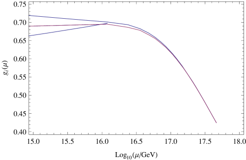
Suppose a Higgs superpotential which provides the same VEVs ($v_{\rm PS}$) for Higgs multiplets to break the PS symmetry and leaves only the particle contents of the minimal supersymmetric Standard Model (MSSM) at low energies. In Ref. [12], assuming $M_{c}=v_{\rm PS}$ and imposing the left-right symmetry, the gauge coupling unification was examined. Analyzing the gauge coupling runnings in the MSSM, $M_{c}=v_{\rm PS}$ is fixed as the scale where the SU(2)_L and SU(2)_R gauge couplings coincide with each other, which is found to be $M_{c}=v_{\rm PS}=1.2\times 10^{16}$ GeV. For the scale $\mu\geq M_{c}=v_{\rm PS}$, we have only two independent gauge couplings, SU(4)_c and SU(2)_L (or SU(2)_R) gauge couplings. After taking KK mode contributions into account, it was shown that the gauge coupling is successfully unified at $M_{\rm GUT}=4.6\times 10^{17}$ GeV (see Figure 1 from Ref. [12]). We assume that a more fundamental SO(10) GUT theory takes place at $M_{GUT}$, and it would be natural to assume $M_{GUT}\sim M_{5}$. In fact, the relation between 4D and 5D Planck scales, $M_{5}^{3}/M_{c}\simeq M_{P}^{2}$ ($M_{P}=2.44\times 10^{18}$ GeV is the reduced Planck scale), supports this assumption with $M_{c}=1.2\times 10^{16}$ GeV. When we abandon the left-right symmetry, there is more freedom for the gauge coupling unification with two independent parameters $v_{PS}$ and $M_{c}$.

Our model gives a large $v_{PS}$ relative to other 5D orbifold SO(10) models [11]. The high value of $v_{PS}$ or $M_{c}$ is advantageous for dangerous proton decay due to dimension six operators. From Eq. (2), the right-handed neutrino mass scale is given by $M_{R}\sim Y_{R}v_{PS}^{2}/M_{5}\sim Y_{R}v_{PS}^{2}/M_{\rm GUT}$. The scale $M_{R}={\cal O}(10^{14}~{}\mbox{GeV})$ preferable for the seesaw mechanism can be obtained by a mild tuning of the Yukawa coupling $Y_{R}\sim 0.1$.

In the next section, we show that this model is well fitted to the smooth hybrid inflation model and the model predictions are compatible with the cosmological observations like the power spectrum of the curvature perturbations, the scalar spectral index, the ratio of scalar-to-tensor fluctuations and so on.

3 Smooth hybrid inflation

We consider the smooth hybrid inflation model [18] in the context of the orbifold GUT model discussed in the previous section. For this purpose, we introduce a singlet chiral superfield $S$. Needless to say, this singlet field causes no change for the gauge coupling unification. Let us consider the superpotential for the smooth hybrid inflation [18],

$$W=S\left(-\mu^{2}+\frac{(\bar{\phi}\phi)^{2}}{M^{2}}\right),$$ (3)

where we have omitted possible ${\cal O}(1)$ coefficients. SUSY vacuum conditions lead to non-zero VEVs for $\langle\phi\rangle=\langle\bar{\phi}\rangle=\sqrt{\mu M}$, by which the PS symmetry is broken down to the SM one, and thus

$$v_{\rm PS}=\sqrt{\mu M}.$$ (4)

In the following analysis of inflation, we treat $M$ as a free parameter with $v_{\rm PS}=\sqrt{\mu M}=1.2\times 10^{16}$ GeV fixed by the analysis of gauge coupling unification. Since $M$ is involved in the non-renormalizable term, it is theoretically natural that $M\sim M_{5}\sim M_{\rm GUT}=4.6\times 10^{17}$ GeV. Nevertheless this condition is independent of the inflation scenario, we will find from the following analysis that $M\sim M_{\rm GUT}$ is in fact consistent with the cosmological observations. Therefore, our GUT model is suitable for the inflation models with the parameters $v_{\rm PS}$ and $M_{\rm GUT}$ fixed by the analysis for the gauge coupling unification.

There are many possibility of the other parts of Higgs superpotential involving other Higgs multiplets in Table 2. See, for example, Ref. [12] and also the Higgs superpotential in Ref. [17]. It would be worth mentioning that the Higgs superpotential includes a term $W\supset H_{6}(\phi^{2}+\bar{\phi}^{2})$ through which all color triplets in $\phi$ and $\bar{\phi}$ become heavy. Only the superpotential of Eq. (3) is relevant for inflation.

Now we examine the smooth hybrid inflation scenario. The scalar potential from Eq. (3) is given by

$$V=\left|-\mu^{2}+\frac{(\bar{\phi}\phi)^{2}}{M^{2}}\right|^{2}+4S^{2}\frac{|\phi|^{2}|\bar{\phi}|^{2}}{M^{4}}\left(|\phi|^{2}+|\bar{\phi}|^{2}\right).$$ (5)

Considering the D-flatness condition, we normalize

$$|\phi|=|\bar{\phi}|=\frac{\chi}{2},~{}~{}|S|=\frac{\sigma}{\sqrt{2}}$$ (6)

and then V becomes

$$V=\left(\mu^{2}-\frac{\chi^{4}}{16M^{2}}\right)^{2}+\frac{\chi^{6}\sigma^{2}}{16M^{4}}.$$ (7)

For a fixed $\sigma$, $V$ has a minimum at

$$\chi^{2}=-6\sigma^{2}+\sqrt{36\sigma^{4}+16v_{\rm PS}^{4}}\simeq\frac{4}{3}\frac{v_{\rm PS}^{4}}{\sigma^{2}},$$ (8)

where we have used an approximation for $\sigma^{2}\gg v_{PS}^{2}$ (satisfied during inflation) in the last expression. The inflation trajectory is along this minimum and we obtain the potential along this path

$$V\simeq\mu^{4}\left(1-\frac{2v_{\rm PS}^{4}}{27\sigma^{4}}\right).$$ (9)

Note that the PS symmetry is spontaneously broken anywhere on the inflation trajectory and thus, no topological defects such as strings, monopoles, or domain walls are produced at the end of inflation [18].

Accordingly, the slow-roll parameters ($\epsilon$, $\eta$) and the parameter ($\xi^{2}$), which enters the running of the spectral index, are defined as [20]

$$\epsilon = \frac{M_{P}^{2}}{2}\left(\frac{V^{\prime}}{V}\right)^{2}\simeq\frac{32M_{P}^{2}v_{\rm PS}^{8}}{729\sigma^{10}}\simeq-\frac{4v_{\rm PS}^{4}}{135\sigma^{4}}\eta$$

$$\eta = M_{P}^{2}\left(\frac{V^{\prime\prime}}{V}\right)=-\frac{40M_{P}^{2}v_{\rm PS}^{4}}{27\sigma^{6}}$$

$$\xi^{2} = M_{P}^{4}\left(\frac{V^{\prime}V^{\prime\prime\prime}}{V^{2}}\right)\simeq\frac{640M_{P}^{4}v_{\rm PS}^{8}}{243\sigma^{12}},$$ (10)

where the prime denotes derivative with respect to $\sigma$. The slow-roll approximation is valid if the conditions, $\epsilon$ and $|\eta|\ll 1$, hold. In this case, the spectral index ($n_{\rm s}$), the ratio of tensor-to-scalar fluctuations ($r$) and the running of the spectral index ($\alpha_{\rm s}$) are given by

$$n_{\rm s} \simeq 1-6\epsilon+2\eta,$$

$$r \simeq 16\epsilon,$$

$$\alpha_{\rm s} = \frac{dn_{\rm s}}{d\ln k}\simeq 16\epsilon\eta-24\epsilon^{2}-2\xi^{2}.$$ (11)

The number of e-folds $N_{k}$ after the comoving scale $\ell_{0}=2\pi/k_{0}$ has crosses the horizon is given by

$$N_{k}=\frac{1}{M_{P}^{2}}\int^{\sigma_{k}}_{\sigma_{f}}d\sigma\frac{V}{V^{\prime}}\simeq\frac{9}{16M_{P}^{2}v_{\rm PS}^{4}}\left(\sigma_{k}^{6}-\sigma_{f}^{6}\right),$$ (12)

where $\sigma_{k}$ is the value of the inflaton field when the scale corresponding to $k_{0}$ exits the horizon, and $\sigma_{f}$ is the value of the inflaton field when the inflation ends, which is determined by $|\eta|=1$ so that

$$\sigma_{f}^{6} = \frac{40}{27}M_{P}^{2}v_{\rm PS}^{4}.$$ (13)

For $\sigma_{k}^{6}\gg\sigma_{f}^{6}$, several formulas given above are reduced into simpler forms, for example,

$$N_{k}\simeq-\frac{5}{6\eta_{k}},~{}~{}n_{s}\simeq 1-\frac{5}{3N_{k}},~{}~{}\alpha_{\rm s}\simeq-\frac{5}{3N_{k}^{2}}.$$ (14)

The number of e-folds $N_{k}$ required for solving the horizon and flatness problems of the standard big bang cosmology, for $k_{0}=0.002$ Mpc^-1, is given by [20]

$$N_{k}\simeq 51.4+\frac{2}{3}\ln\left(\frac{V(\sigma_{k})^{1/4}}{10^{15}~{}{\rm GeV}}\right)+\frac{1}{3}\ln\left(\frac{T_{\rm rh}}{10^{7}~{}{\rm GeV}}\right),$$ (15)

where we have assumed a standard thermal history, and $T_{\rm rh}$ is the reheating temperature after inflation. If gravitino has mass around 100 GeV as in the gravity mediated SUSY breaking, the reheating temperature is severely constraint (gravitino problem) in order for the gravitino decay products not to destroy the light elements successfully synthesized during big bang nucleosynthesis [21],

$$T_{\rm rh}\leq 10^{6}-10^{7}\textrm{GeV}.$$ (16)

The power spectrum of the primordial curvature perturbation at the scale $k_{0}$ is given by

$${\cal{P_{R}}}^{1/2}\simeq\frac{1}{2\sqrt{3}\pi M_{P}^{3}}\frac{V^{3/2}}{|V^{\prime}|}\simeq\frac{27}{16\sqrt{3}\pi}\frac{\sigma_{k}^{5}}{M_{P}^{3}M^{2}}.$$ (17)

This should satisfy the observed value by the WMAP [22], ${\cal{P_{R}}}\simeq 2.457\times 10^{-9}$.

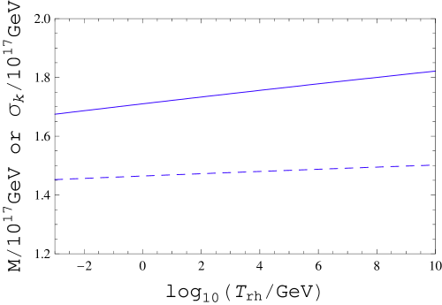
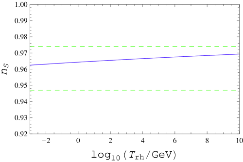
Now we solve Eqs. (12), (15) and (17) and fix the model parameters involving the inflation scenario. In our analysis, we have three independent free parameters, $M$, $\sigma_{k}$ and $T_{\rm rh}$, with the fixed $v_{\rm PS}=1.2\times 10^{16}$ GeV. We solve the equations for a given $T_{\rm rh}$ in the range 1 MeV $\leq T_{\rm rh}\leq 10^{10}$ GeV and find $M$ and $\sigma_{k}$. Figure 2 shows the results for $M$ and $\sigma_{k}$ as a function of $T_{\rm rh}$. We can check that $\sigma_{k}^{6}\gg\sigma_{f}^{6}$ and the slow-roll conditions are satisfied. The number of e-folds is depicted in Figure 3. Using these outputs and Eq. (10), we evaluate the spectral index (Figure 4), the tensor-to-scalar ratio and the running of the spectral index:

$$0.963\leq n_{\rm s} \leq 0.968,$$

$$4.0\times 10^{-7}\geq r \geq 3.1\times 10^{-7},$$

$$-8.4\times 10^{-4}\leq \alpha_{\rm s} \leq-6.1\times 10^{-4}$$ (18)

for 1 MeV $\leq T_{\rm rh}\leq 10^{7}$ GeV. The tensor-to-scalar ratio and the running of the spectral index are negligibly small. These results are consistent with the WMAP 5-year data [22]: $n_{\rm s}=0.960^{+0.014}_{-0.013}$, $r<0.2$ (95% CL) and $\alpha_{\rm s}=-0.032^{+0.021}_{-0.020}$ (68% CL) (consistent with zero in 95% CL).

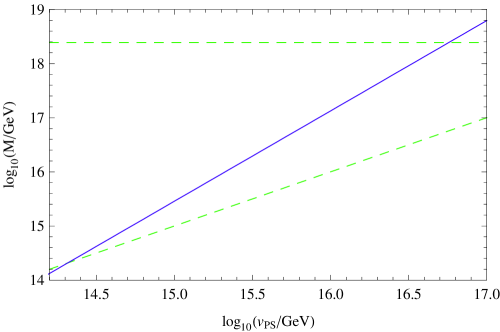
In general, we do not need to impose either the left-right symmetry or $M_{c}=v_{\rm PS}$ on the model. In this case, $v_{\rm PS}$ can be varied [11], and we repeat the same analysis for this general case with $v_{\rm PS}$ as a free parameter. Fixing, for example, $T_{\rm rh}=10^{7}$ GeV, $M$ can be obtained as a function of $v_{\rm PS}$ as shown in Figure 5. Since $M$ appears in the non-renormalizable term, it would be natural to identify $M$ as an effective cutoff. Thus, the theoretical consistency leads to the condition, $v_{\rm PS}\leq M\leq M_{P}$, from which we obtain $1.9\times 10^{14}$ GeV $\leq v_{\rm PS}\leq 5.6\times 10^{16}$ GeV. The number of e-folds and the tensor-to-scalar ratio are shown in Figure 6 and 7, respectively, as a function of $v_{\rm PS}$. The other outputs, the spectral index and its running, are found as

$$0.967\leq n_{\rm s} \leq 0.968,$$

$$-6.4\times 10^{-4}\leq \alpha_{\rm s} \leq-6.1\times 10^{-4}.$$ (19)

These are consistent with the WMAP data.

4 Conclusions

We have discussed the smooth hybrid inflation scenario in the context of the SO(10) GUT model in Ref. [12]. We have shown that the model can be naturally applicable to the inflation model by introducing only one singlet chiral multiplet, keeping the structure of the gauge coupling unification unchanged. The analysis for the running gauge coupling fixes the model parameters as $v_{\rm PS}=1.2\times 10^{16}$ GeV and $M_{\rm GUT}=4.6\times 10^{17}$ GeV. It is very interesting that these parameters are determined independently of the cosmological considerations, nevertheless the inflation scenario with these parameters fits very well with the current cosmological observations, as we have shown.

Figure 1: Gauge coupling unification in the left-right symmetric case, taken from Ref. [12]. Each line from top to bottom corresponds to $g_{3}$, $g_{2}$ and $g_{1}$ for $\mu<M_{c}=v_{\rm PS}$, while $g_{3}=g_{4}$ and $g_{2}=g_{2R}$ for $\mu>M_{c}=v_{\rm PS}$.

Figure 2: $M$ and $\sigma_{k}$ as a function of $T_{\rm rh}$. The solid and dashed lines correspond to $M$ and $\sigma_{k}$, respectively.

Figure 3: The number of e-folds versus $T_{\rm rh}$.

Figure 4: The spectral index as a function of $T_{\rm rh}$. The dashed lines correspond to the WMAP 5-year data, $n_{\rm s}=0.960^{+0.014}_{-0.013}$.

Figure 5: $M$ as a function of $v_{\rm PS}$ (solid line). The lower and upper dashed lines specified the theoretical consist region for $M$, $v_{\rm PS}\leq M\leq M_{P}$.

Figure 6: The number of e-folds versus $v_{\rm PS}$.

Figure 7: The tensor-to-scalar ratio versus $v_{\rm PS}$.

References

- [1] K. S. Babu and R. N. Mohapatra, Phys. Rev. Lett. 70, 2845 (1993).
- [2] K. Matsuda, Y. Koide and T. Fukuyama, Phys. Rev. D 64, 053015 (2001); K. Matsuda, Y. Koide, T. Fukuyama and H. Nishiura, Phys. Rev. D 65, 033008 (2002) [Erratum-ibid. D 65, 079904 (2002)].
- [3] T. Fukuyama and N. Okada, JHEP 0211, 011 (2002).
- [4] K. Eguchi et al. [KamLAND Collaboration], Phys. Rev. Lett. 90, 021802 (2003).
- [5] T. Fukuyama, A. Ilakovac, T. Kikuchi, S. Meljanac and N. Okada, Eur. Phys. J. C 42, 191 (2005); ibid., J. Math. Phys. 46, 033505 (2005); Phys. Rev. D 72, 051701 (2005).
- [6] B. Bajc, A. Melfo, G. Senjanović and F. Vissani, Phys. Rev. D 70, 035007 (2004).
- [7] S. Bertolini, T. Schwetz and M. Malinsky, Phys. Rev. D 73, 115012 (2006).
- [8] T. Fukuyama, T. Kikuchi and N. Okada, Phys. Rev. D 75, 075020 (2007); R. N. Mohapatra, N. Okada and H. B. Yu, Phys. Rev. D 76 015013 (2007).
- [9] L. Randall and R. Sundrum, Phys. Rev. Lett. 83, 3370 (1999).
- [10] Y. Kawamura, Prog. Theor. Phys. 105, 999 (2001); . G. Altarelli and F. Feruglio, Phys. Lett. B 511, 257 (2001); A. B. Kobakhidze, Phys. Lett. B 514, 131 (2001); . L. Hall and Y. Nomura, Phys. Rev. D 64 055003 (2001); A. Hebecker and J. March-Russell, Nucl. Phys. B 613, 3 (2001).
- [11] R. Dermisek and A. Mafi, Phys. Rev. D 65, 055002 (2002); H. D. Kim and S. Raby, JHEP 0301 056 (2003); S. M. Barr and I. Dorsner, Phys. Rev. D 66, 065013 (2002); I. Dorsner, Phys. Rev. D 69, 056003 (2004); B. Kyae, C. A. Lee and Q. Shafi, Nucl. Phys. B 683, 105 (2004); M. L. Alciati and Y. Lin, JHEP 0509 (2005) 061; M. L. Alciati, F. Feruglio, Y. Lin and A. Varagnolo, JHEP 0611 (2006) 039.
- [12] T. Fukuyama and N. Okada, arXiv:0803.1758 [hep-ph], to be published in Phys. Rev. D.
- [13] A. D. Linde, Phys. Rev. D 49, 748 (1994).
- [14] For a review, see, for example, G. Lazarides, arXiv:hep-ph/0011130; C. Pallis, arXiv:0710.3074 [hep-ph], and references therein.
- [15] E. J. Copeland, A. R. Liddle, D. H. Lyth, E. D. Stewart and D. Wands, Phys. Rev. D 49, 6410 (1994).
- [16] G. R. Dvali, Q. Shafi and R. K. Schaefer, Phys. Rev. Lett. 73, 1886 (1994); G. Lazarides, R. K. Schaefer and Q. Shafi, Phys. Rev. D 56, 1324 (1997).
- [17] R. Jeannerot, S. Khalil, G. Lazarides and Q. Shafi, JHEP 0010, 012 (2000); R. Jeannerot, S. Khalil and G. Lazarides, JHEP 0207, 069 (2002).
- [18] G. Lazarides and C. Panagiotakopoulos, Phys. Rev. D 52, 559 (1995); G. Lazarides, C. Panagiotakopoulos and N. D. Vlachos, Phys. Rev. D 54, 1369 (1996); G. Lazarides and A. Vamvasakis, Phys. Rev. D 76, 083507 (2007).
- [19] A. D. Linde and A. Riotto, Phys. Rev. D 56, 1841 (1997); V. N. Senoguz and Q. Shafi, Phys. Lett. B 567, 79 (2003).
- [20] For a review, see, for example, D. H. Lyth and A. Riotto, Phys. Rept. 314, 1 (1999), and references therein; Liddle A R and Lyth D H, Cosmological Inflation and Large-Scale Structure, Cambridge University Press (2000). G. Lazarides, Lect. Notes Phys. 592, 351 (2002); J. Phys. Conf. Ser. 53, 528 (2006).
- [21] For recent analysis, see, for example, R. H. Cyburt, J. R. Ellis, B. D. Fields and K. A. Olive, Phys. Rev. D 67, 103521 (2003); M. Kawasaki, K. Kohri and T. Moroi, Phys. Lett. B 625, 7 (2005).
- [22] G. Hinshaw et al. [WMAP Collaboration], arXiv:0803.0732 [astro-ph].