A New Causal Interpretation of EPR-B Experiment

Abstract

In this paper we study a two-step version of EPR-B experiment, the Bohm version of the Einstein-Podolsky-Rosen experiment. Its theoretical resolution in space and time enables us to refute the classic "impossibility" to decompose a pair of entangled atoms into two distinct states, one for each atom. We propose a new causal interpretation of the EPR-B experiment where each atom has a position and a spin while the singlet wave function verifies the two-body Pauli equation. In conclusion we suggest a physical explanation of non-local influences, compatible with Einstein’s point of view on relativity.

keywords: EPR-B - causal interpretation - entangled atoms - two-body Pauli equation - singlet state

1 Introduction

The nonseparability is one of the most puzzling aspects of quantum mechanics. For over thirty years, the EPR-B, the spin version proposed by Bohm [5, 6] of the Einstein-Podolsky-Rosen experiment [1], the Bell theorem [2] and the BCHSH inequalities [2, 3, 4] have been at the heart of the debate on hidden variables and non-locality; but hitherto the precise nature of the physical process that lies behind the "non-local" correlations in the spins of the particles has remained unclear.

Many experiments since Bell’s paper have demonstrated violations of these inequalities and have vindicated quantum theory [7, 8, 9, 10, 11, 12, 13, 14, 15, 16, 17]. The first one was done with pairs of entangled photons and clearly violate Bell’s inequality [10, 11, 12, 13]. Entangled protons have also been studied in an early experiment [9]. The generation of EPR pairs of massive atoms instead of massless photons has been considered [14, 15]; it also shows experimental violation of Bell’s inequality with efficient detection [15].

In a new experiment, Zeilinger and all [26] measure previously untested correlations between two entangled photons, they show that these correlations violate an inequality proposed by Leggett for non-local realistic theories [25].

The usual conclusion of these experiments is to reject the non-local realism because the impossibility to decompose a pair of entangled atoms into two states, one for each atom.

In this paper we show, on the EPR-B experiment, that this decomposition is possible: a causal interpretation exists where each atom has a position and a spin while the singlet wave function verifies the two-body Pauli equation.

To demonstrate this; we consider a two-step version of EPR-B experiment and we use an analytic expression of the wave function and the probability density. The explicit solution is obtained via a complete integration of the two-body Pauli equation over time and space.

A first causal interpretation of EPR-B experiment was proposed in 1987 by Dewdney, Holland and Kyprianidis [21, 22]. This interpretation had a flaw: the spin of each particle depends directly on the singlet wave function, and so the spin module of each particle varied during the experiment from 0 to $\frac{\hbar}{2}$.

The explicit solution in terms of two-body Pauli spinors and the probability density for the two steps of the EPR-B experiment are presented in section 2. The solution in space and time shows how it is possible to deduce tests on the spatial quantization of particles, similar to those of the Stern and Gerlach experiment.

In section 3, we provide a realistic explanation of the entangled states and a method to desentangle the wave function of the two particles.

The resolution in space of the equation Pauli is essential: it enables the spatial quantization in section 2 and explains determinism and desentangling in section 3.

In conclusion we propose a physical explanation of non-local influences, compatible with Einstein’s point of view on relativity.

2 Simulation and tests of EPR-B experiment in two steps

Fig.1 presents the Einstein-Podolsky-Rosen-Bohm experiment. A source $S$ created in O pairs of identical atoms A and B, but with opposite spins. The atoms A and B split following 0y axis in opposite directions, and head towards two identical Stern-Gerlach apparatus $\mathcal{A}$ and $\mathcal{B}$.

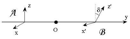
Figure 1: Schematic configuration of EPR-B experiment.

The electromagnet $\mathcal{A}$ "measures" the A spin in the direction of the Oz-axis and the electromagnet $\mathcal{B}$ "measures" the B spin in the direction of the Oz’-axis, which is obtained after a rotation of an angle $\delta$ around the Oy-axis.

We further consider that atoms A and B may be represented by Gaussian wave packets in x and z. We note $\textbf{r}=(x,z)$. The initial wave function of the entangled state is the singlet state:

$$\Psi_{0}(\textbf{r}_{A},\textbf{r}_{B})=\frac{1}{\sqrt{2}}f(\textbf{r}_{A})f(\textbf{r}_{B})(|+_{A}\rangle|-_{B}\rangle-|-_{A}\rangle|+_{B}\rangle)$$ (1)

where $f(\textbf{r})=(2\pi\sigma_{0}^{2})^{-\frac{1}{2}}e^{-\frac{x^{2}+z^{2}}{4\sigma_{0}^{2}}}$ and where $|\pm_{A}\rangle$ ($|\pm_{B}\rangle$) are the eigenvectors of the spin operators $\widehat{s}_{z_{A}}$ ($\widehat{s}_{z_{B}}$) in the z-direction pertaining to particule A (B): $\widehat{s}_{z_{A}}|\pm_{A}\rangle=\pm(\frac{\hbar}{2})|\pm_{A}\rangle$ ($\widehat{s}_{z_{B}}|\pm_{B}\rangle=\pm(\frac{\hbar}{2})|\pm_{B}\rangle$). We treat classically dependence with y: speed $-v_{y}$ for A and $v_{y}$ for B.

The wave function $\Psi(\textbf{r}_{A},\textbf{r}_{B},t)$ of the two identical particles A and B, electrically neutral and with magnetic moments $\mu_{0}$, subject to magnetic fields $\textbf{B}^{\mathcal{A}}$ and $\textbf{B}^{\mathcal{B}}$, admits in the basis $|\pm_{A}\rangle$ and $|\pm_{B}\rangle$ 4 components $\Psi^{a,b}(\textbf{r}_{A},\textbf{r}_{B},t)$ and verifies the two-body Pauli equation [24] p. 417:

$$i\hbar\frac{\partial\Psi^{a,b}}{\partial t}=\left(-\frac{\hbar^{2}}{2m}\Delta_{A}-\frac{\hbar^{2}}{2m}\Delta_{B}\right)\Psi^{a,b}+\mu B^{\mathcal{A}}_{j}(\sigma_{j})_{c}^{a}\Psi^{c,b}+\mu B^{\mathcal{B}}_{j}(\sigma_{j})_{d}^{b}\Psi^{a,d}$$ (2)

with the initial conditions:

$$\Psi^{a,b}(\textbf{r}_{A},\textbf{r}_{B},0)=\Psi_{0}^{a,b}(\textbf{r}_{A},\textbf{r}_{B})$$ (3)

where the $\sigma_{j}$ are the Pauli matrixes and where the $\Psi_{0}^{a,b}(\textbf{r}_{A},\textbf{r}_{B})$ correspond to the singlet state (1).

We take as numerical values those of the Stern-Gerlach experiment with silver atoms [18, 19]. For a silver atom, one has $m=1,8\times 10^{-25}$ kg, $v_{y}=500$ m/s , $\sigma_{0}$=10^-4m. For the electromagnetic field B, $B_{x}=B^{\prime}_{0}x$; $B_{y}=0$ and $B_{z}=B_{0}-B^{\prime}_{0}z$ with $B_{0}=5$ Tesla, $B^{\prime}_{0}=\left|\frac{\partial B}{\partial z}\right|=-\left|\frac{\partial B}{\partial x}\right|=10^{3}$ Tesla/m over a length $\Delta l=1~{}cm$. The screen that intercepts atoms is at a distance $D=20~{}cm$ (time $t_{1}=\frac{D}{v_{y}}=4\times 10^{-4}$s) from the exit of the magnetic field.

One of the difficulties of the interpretation of the EPR-B experiment is the existence of two simultaneous measurements. By doing these measurements one after the other, the interpretation of the experiment will be facilitated. That is the purpose of the two-step version of the experiment EPR-B studied below.

2.1 First step: Measurement of A spin and position of B

In the first step we make, on a couple of particles A and B in a singlet state, a Stern and Gerlach "measurement" for atom A, and for atom B a mere impact measurement on a screen.

It is the experiment first proposed in 1987 by Dewdney, Holland and Kyprianidis [21].

Consider that at time $t_{0}$ the particle A arrives at the entrance of electromagnet $\mathcal{A}$. $\triangle t$ is the crossing duration of electromagnet $\mathcal{A}$ and $t$ is the time after the $\mathcal{A}$ exit. The wave function can be calculated, from the wave function (1), term to term in basis [$|\pm_{A}\rangle,|\pm_{B}\rangle$]. After this exit of the magnetic field $\mathcal{A}$, at time $t_{0}+\triangle t+t$, the wave function (1) becomes [19]:

$$\Psi(\textbf{r}_{A},\textbf{r}_{B},t_{0}+\triangle t+t) = \frac{1}{\sqrt{2}}f(\textbf{r}_{B})$$

$$\times\left(f^{+}(\textbf{r}_{A},t)|+_{A}\rangle|-_{B}\rangle-f^{-}(\textbf{r}_{A},t)|-_{A}\rangle|+_{B}\rangle\right)$$

with

$$f^{\pm}(\textbf{r},t)\simeq f(x,z\mp z_{\triangle}\mp ut)e^{i(\frac{\pm muz}{\hbar}+\varphi^{\pm}(t))}$$ (5)

and

$$\Delta t=\frac{\Delta l}{v_{y}}= 2\times 10^{-5}s,~{}~{}~{}~{}z_{\Delta}=\frac{\mu_{0}B^{\prime}_{0}(\Delta t)^{2}}{2m}=10^{-5}m,$$ (6)

$$u=\frac{\mu_{0}B^{\prime}_{0}(\Delta t)}{m}=1m/s.$$

The atomic density $\rho(z_{A},z_{B},t_{0}+\Delta t+t)$ is found by integrating $\Psi^{*}(\textbf{r}_{A},\textbf{r}_{B},t_{0}+\triangle t+t)\Psi(\textbf{r}_{A},\textbf{r}_{B},t_{0}+\triangle t+t)$ on $x_{A}$ and $x_{B}$:

$$\rho(z_{A},z_{B},t_{0}+\Delta t+t) = \left((2\pi\sigma_{0}^{2})^{-\frac{1}{2}}e^{-\frac{(z_{B})^{2}}{2\sigma_{0}^{2}}}\right)$$

$$\times\left((2\pi\sigma_{0}^{2})^{-\frac{1}{2}}\frac{1}{2}\left(e^{-\frac{(z_{A}-z_{\Delta}-ut)^{2}}{2\sigma_{0}^{2}}}+e^{-\frac{(z_{A}+z_{\Delta}+ut)^{2}}{2\sigma_{0}^{2}}}\right)\right).$$

We deduce that the beam of particles A is divided into two, while the B beam of particle stays one. This result can easily be tested experimentally.

Moreover, we note that the space quantization of particle A is identical to that of an untangled particle in a Stern and Gerlach apparatus: the distance $\delta z=2(z_{\Delta}+ut)$ between the two spots $N^{+}$ (spin +) and $N^{-}$ (spin $-$) of a family of particle A is the same as the distance between the two spots $N^{+}$ and $N^{-}$ of a particle in a classic Stern and Gerlach experiment [19]. This result can easily be tested experimentally.

We finally deduce from (2.1) that:

• the density of A is the same, whether particle A is entangled with B or not,

• the density of B is not affected by the "measurement" of A.

These two predictions of quantum mechanics can be tested. Only spins are involved. We conclude from (2.1) that the spins of A and B remain opposite throughout the experiment.

2.2 Second step: "Measurement" of A spin, then of B spin.

The second step is a continuation of the first and results in realizing the EPR-B experiment in two steps.

On a couple of particles A and B in a singlet state, first we made a Stern and Gerlach "measurement" on the A atom between $t_{0}$ and $t_{0}+\triangle t+t_{1}$, then a Stern and Gerlach "measurement" on the B atom with an electromagnet $\mathcal{B}$ forming an angle $\delta$ with $\mathcal{A}$ between $t_{0}+\triangle t+t_{1}$ and $t_{0}+2(\triangle t+t_{1})$.

Beyond the exit of magnetic field $\mathcal{A}$, at time $t_{0}+\triangle t+t_{1}$, the wave function is given by (2.1). Immediately after the "measurement" of A, still at time $t_{0}+\triangle t+t_{1}$, if the A measurement is $\pm$, the conditionnal wave functions of B are:

$$\Psi_{B/\pm A}(\textbf{r}_{B},t_{0}+\triangle t+t_{1})=f(\textbf{r}_{B})|\mp_{B}\rangle.$$ (8)

To measure B, we refer to the basis $|\pm^{\prime}_{B}\rangle$ where $|\pm^{\prime}_{B}\rangle$ are the eigenvectors of the spin operators $\widehat{s}_{z^{\prime}_{B}}$ in the z’-direction pertaining to particule B. We note $\textbf{r}^{\prime}=(x^{\prime},z^{\prime})$. So, after the measurement of B, at time $t_{0}+2(\triangle t+t_{1})$ the conditional wave functions of B are:

$$\Psi_{B/+A}(\textbf{r}^{\prime}_{B},t_{0}+2(\triangle t+t_{1}))=\cos\frac{\delta}{2}f^{+}(\textbf{r}^{\prime}_{B},t_{1})|+^{\prime}_{B}\rangle+\sin\frac{\delta}{2}f^{-}(\textbf{r}^{\prime}_{B},t_{1})|-^{\prime}_{B}\rangle,$$ (9)

$$\Psi_{B/-A}(\textbf{r}^{\prime}_{B},t_{0}+2(\triangle t+t_{1}))=-\sin\frac{\delta}{2}f^{+}(\textbf{r}^{\prime}_{B},t_{1})|+^{\prime}_{B}\rangle+\cos\frac{\delta}{2}f^{-}(\textbf{r}^{\prime}_{B},t_{1})|-^{\prime}_{B}\rangle.$$ (10)

We therefore obtain, in this two steps version of the EPR-B experiment, the same results for spatial quantization and correlations of spins as in the EPR-B experiment.

3 Causal interpretation of the EPR-B experiment

We assume, at moment of the creation of the two entangled particles A and B, that each of the two particles A and B has an initial wave function $\Psi_{0}^{A}(\textbf{r}_{A},\theta^{A}_{0},\varphi^{A}_{0})$ and $\Psi_{0}^{B}(\textbf{r}_{B},\theta^{B}_{0},\varphi^{B}_{0})$ with spinors which are opposite spins; for example
$\Psi_{0}^{A}(\textbf{r}_{A},\theta^{A}_{0},\varphi^{A}_{0})=f(\textbf{r}_{A})\left(\cos\frac{\theta^{A}_{0}}{2}|+_{A}\rangle+\sin\frac{\theta^{A}_{0}}{2}e^{i\varphi^{A}_{0}}|-_{A}\rangle\right)$ and
$\Psi_{0}^{B}(\textbf{r}_{B},\theta^{B}_{0},\varphi^{B}_{0})=f(\textbf{r}_{B})\left(\cos\frac{\theta^{B}_{0}}{2}|+_{B}\rangle+\sin\frac{\theta^{B}_{0}}{2}e^{i\varphi^{B}_{0}}|-_{B}\rangle\right)$ with $\theta_{0}^{B}=\pi-\theta_{0}^{A}$ and $\varphi_{0}^{B}=\varphi_{0}^{A}-\pi$.

Then the Pauli principle tells us that the two-body wave function must be antisymmetric; after calculation we find:

$$\Psi_{0}(\textbf{r}_{A},\theta^{A},\varphi^{A},\textbf{r}_{B},\theta^{B},\varphi^{B})=-e^{i\varphi^{A}}f(\textbf{r}_{A})f(\textbf{r}_{B})\times\left(|+_{A}\rangle|-_{B}\rangle-|-_{A}\rangle|+_{B}\rangle\right)$$

which is the same as the singlet state, factor wise (1).

Thus, we can consider that the singlet wave function is the wave function of a family of two fermions A and B with opposite spins: direction of initial spin A and B exist, but is not known. It is a local hidden variable which is therefore necessary to add in the initial conditions of the model.

This is not the interpretation followed by the school of Bohm  [21, 22, 24, 23] in the interpretation of the singlet wave function; they suppose, for example, a zero spin for each of particles A and B at the initial time.

It remains to determine the wave function and the trajectories of particles A and B: from the entangled wave function, initial spins and initial positions of each particle.

We assume therefore that the intial position of the particle A is known ($x_{0}^{A},y_{0}^{A}=0,z_{0}^{A})$ as well as the particle B ($x_{0}^{B}=x_{0}^{A}$,$y_{0}^{B}=y_{0}^{A}=0$,$z_{0}^{B}=z_{0}^{A}$).

3.1 Step 1: Measurement of A spin and position of B

Equation (2.1) shows that the spins of A and B remain opposite throughout step 1. Equation (2.1) shows that the densities of A and B are independent; for A equal to the density of a family of free particles in a classical Stern Gerlach apparatus, whose initial spin orientation has been randomly chosen; for B equal to the density of a family of free particles.

The spin of a particle A is orientated gradually following the position of the particle in its wave into a spin $+$ or $-$. The spin of particle B follows that of A, while remaining opposite.

In the equation (2.1) particle A can be considerd independent of B. We can therefore give it the wave function

$$\Psi^{A}(\textbf{r}_{A},t_{0}+\triangle t+t)=\cos\frac{\theta_{0}^{A}}{2}f^{+}(\textbf{r}_{A},t)|+_{A}\rangle+\sin\frac{\theta_{0}^{A}}{2}e^{i\varphi_{0}^{A}}f^{-}(\textbf{r}_{A},t)|-_{A}\rangle$$ (11)

which is that of a free particle in a Stern Gerlach apparatus and whose initial spin is given by ($\theta_{0}^{A},\varphi_{0}^{A}$).

In de Broglie interpretation [23], particle velocity is proportional to the gradient of the wave function phase. See compute exemples for Young experiment [20] and Stern-Gerlach experiment [19]. So, the equation of its trajectory is given by the following differential equations: in the interval $[t_{0},t_{0}+\Delta t]$:

$$\frac{dz_{A}}{dt}=\frac{\mu_{0}B^{\prime}_{0}t}{m}cos\theta(z_{A},t)$$ (12)

with $$\tan\frac{\theta(z_{A},t)}{2}=\tan\frac{\theta_{0}}{2}e^{-\frac{\mu_{0}B^{\prime}_{0}t^{2}z_{A}}{2m\sigma_{0}^{2}}}$$

with the initial condition $z_{A}(t_{0})=z^{A}_{0}$; and in the interval $t_{0}+\Delta t+t$ ($t\geq 0$):

$$\frac{dz_{A}}{dt}=u\frac{\tanh(\frac{(z_{\Delta}+ut)z_{A}}{\sigma_{0}^{2}})+\cos\theta_{0}}{1+\tanh(\frac{(z_{\Delta}+ut)z_{A}}{\sigma_{0}^{2}})\cos\theta_{0}}$$ (13)

et $$\tan\frac{\theta(z_{A}(t),t)}{2}=\tan\frac{\theta_{0}}{2}e^{-\frac{(z_{\Delta}+ut)z_{A}}{\sigma_{0}^{2}}}.$$

$\theta(z_{A}(t),t)$ describes the evolution of the orientation of spin A.

The case of particle B is different. B follows a rectilinear trajectory with $y_{B}(t)=v_{y}t$, $z_{B}(t)=z_{0}^{B}$ and $x_{B}(t)=x_{0}^{B}$. By contrast, the orientation of its spin moves and it was $\theta^{B}(t)=\pi-\theta(z_{A}(t),t)$ and $\varphi^{B}(t)=\varphi(z_{A}(t),t)-\pi$.

We can then associate the wave function:

$$\Psi^{B}(\textbf{r}_{B},t_{0}+\triangle t+t)=f(\textbf{r}_{B})\left(\cos\frac{\theta^{B}(t)}{2}|+_{B}\rangle+\sin\frac{\theta^{B}(t)}{2}e^{i\varphi^{B}(t)}|-_{B}\rangle\right).$$ (14)

This wave funtion is specific, because it depends upon initial conditions of A (positions and spins). The orientation of spin of the particle B is driven by the particle A through the singlet wave function. Thus, the singlet wave function is the actual non-local hidden variable.

Figure 2 presents a plot in the $(z,y)$ plane the trajectories of a set of 5 pairs of entangled atoms whose initial characteristics $(\theta^{A}_{0}=\pi-\theta^{B}_{0},z_{0}^{A}=z_{0}^{B})$ have been randomly chosen. The trajectories will therefore depend on both the initial position $z_{0}$ and the initial spin orientation $\theta_{0}$. Since the spin initial orientation are different, trajectories of the A particles may intersect.

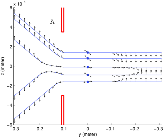
Figure 2: Five pairs of trajectories of entangled particles. Arrows represent the spin orientation ($\theta$).

3.2 Step 2: "Measurement" of A spin, and then B spin

Until time $t_{0}+\triangle t+t_{1}$, we are in the case of step 1. Immediately after the "measurement" of A at the time $t_{0}+\Delta t+t_{1}$, if the A measurement is $\pm$, the conditional wave function of B is given by (8).

Then particle B is in position $(x_{0}^{B},z_{0}^{B})$.

We are exactly in the case of a particle in a Stern and Gerlach magnet $\mathcal{B}$ which is an angle $\delta$ with $\mathcal{A}$.

To measure the spin of B, we refer to the basis $|\pm^{\prime}_{B}\rangle$. So, after the measurement of B, at time $t_{0}+2(\triangle t+t_{1})$, the conditional wave functions of B are given by (9) and (10), and we find again the quantum correlations.

4 Conclusion

From the wave function of two entangled particles, we have determined spins, trajectories and also a wave function for each of the two particles.

In this interpretation, the quantum particle has a local position like a classical particle, but it has also a non local behaviour through the wave function. Indeed the wave function is not separable and non-local. Because in the Broglie-Bohm interpretation the wave function pilots the particle, it also creates the non separability of two entangled particles.

As we saw in step 1, the non-local influence in the EPR-B experiment only concerns the spin orientation, and not the motion of the particles themselves. This is a key point in the search of a physical explanation of non-local influence.

The simplest explanation (Ockham’s razor) of this nonlocal influence is to reintroduce the existence of a space having certain properties related to the action at a distance, that is a kind of ether, but a new form of ether given by Lorentz-Poincaré and then by Einstein in 1920. Einstein said [27]:

"But on the other hand there is a weighty argument to be adduced in favour of the ether hypothesis. To deny the ether is ultimately to assume that empty space has no physical qualities whatever. The fundamental facts of mechanics do not harmonize with this view. For the mechanical behaviour of a corporeal system hovering freely in empty space depends not only on relative positions (distances) and relative velocities, but also on its state of rotation, which physically may be taken as a characteristic not appertaining to the system in itself. In order to be able to look upon the rotation of the system, at least formally, as something real, Newton objectivises space. Since he classes his absolute space together with real things, for him rotation relative to an absolute space is also something real. Newton might no less well have called his absolute space "Ether"; what is essential is merely that besides observable objects, another thing, which is not perceptible, inust be looked upon as real, to enable acceleration or rotation to be looked upon as something real.[…]

Recapitulating, we may say that according to the general theory of relativity space is endowed with physical qualities; in this sense, therefore, there exists an ether. According to the general theory of relativity space without ether is unthinkable; for in such space there not only would be no propagation of light, but also no possibility of existence for standards of space and time (measuring-rods and clocks), nor therefore any space-time intervals in the physical sense. But this ether may not be thought of as endowed with the quality characteristic of ponderable inedia, as consisting of parts which may be tracked through time. The idea of motion may not be applied to it."

Taking into account the new experiments, especially Aspect’s experiments, Popper [28] (p. XVIII) defends a similar view in 1982 :

"I feel not quite convinced that the experiments are correctly interpreted; but if they are, we just have to accept action at a distance. I think (with J.P. Vigier) that this would of course be very important, but I do not for a moment think that it would shake, or even touch, realism. Newton and Lorentz were realists and accepted action at a distance; and Aspect’s experiments would be the first crucial experiment between Lorentz’s and Einstein’s interpretation of the Lorentz transformations."

Lastly, let us notice the great difference between EPR and EPR-B experiments. The spin connected to the rotation of space-time seems to be the cause of the instantaneous action at a distance in experiment EPR-B. It is thus possible that there is not instantaneous action at a distance in original experience EPR. And in this case, Einstein was right. It is the proposal of Popper [28] p.25: " I mays perhaps mention here some of the differences between the original EPR argument and Bohm’version of it. These differences relate to the distinction of two kinds of quantum mechanical state preparations." […] "Indeed, it is possible that the Bohm-Bell experiment decides for action at a distance , and therefore against special relativity theory, whereas the original EPR arguments does not."

The new experiments of non-locality have therefore a great importance, not to eliminate realism and determinism, but as Popper said, to rehabilitate the existence of a certain type of ether, like Lorentz’s ether and like Einstein’s ether in 1920.

References

- [1] Einstein, A., Podolsky, B., Rosen,N.: Can quantum mechanical description of reality be considered complete?. Phys. Rev. 47,777-780 (1935).
- [2] Bell,J. S.: On the Einstein Podolsky Rosen Paradox. Physics 1, 195 (1964).
- [3] Clauser,J.F., Horne,M.A., Shimony, A., Holt,R. A.:Proposed experiments to test local hidden-variable theories. Phys. Rev. Lett. 23, 880 (1969).
- [4] Bell,J. S.: Speakable and Unspeakable in Quantum Mechanics. Cambridge University Press (1987).
- [5] Bohm,D.:Quantum Theory. New York, Prentice-Hall (1951).
- [6] Bohm,D., Aharonov,Y.: Discussion of experimental proofs for the paradox of Einstein, Rosen and Podolsky. Phys. Rev.108, 1070 (1957).
- [7] Freedman, S.J., Clauser,J.F.: Experimental test of local hidden-variable theories. Phys. Rev. Lett. 28, 938 (1972).
- [8] Fry,E. S., Thompson,R.C.: Experimental Test of Local Hidden-Variable Theories. Phys. Rev. Lett. 37, 465 (1976).
- [9] Lamehi-Rachti,M.,Mittig,W.: Phys. Rev. D 14, 2543(1976).
- [10] Aspect,A., Grangier,P., Roger,G.: Experimental realization of Einstein-Pdolsky-Rosen-Bohm GedankenExperiment: a new violation of Bell’inequalities. Phys. Rev. Lett. 49, 91 (1982).
- [11] Aspect,A., Dalibard, J., Roger,G.: Experimental tests of Bell’inequalities using variable analysers. Phys. Rev. Lett. 49, 1804 (1982).
- [12] Tittel,W., Brendel, J., Zbinden, H., Gisin,N.: Violation of Bell inequalities by photons more than 10 km apart. Phys. Rev. Lett. 81, 3563 (1998).
- [13] Weihs,G., Jennewein,T., Simon,C., Weinfurter,H., Zeilinger,A.: Violation of Bell’inequalities under strict Einstein locality condition. Phys. Rev. Lett. 81, 5039 (1998).
- [14] Beige,A., Munro,W.J., Knight,P.L.: A Bell’s inequality test with entangled atoms. Phys. Rev. A 62, 052102-1-052102-9 (2000).
- [15] Rowe,M.A., Kielpinski,D., Meyer, V., Sackett,C.A., Itano,W.M., Monroe,C., Wineland,D.J.: Experimental violation of a Bell’s inequality with efficient detection. Nature 409, 791-794 (2001).
- [16] Bertlmann,R.A., Zeilinger,A. (eds.): Quantum [un]speakables, from Bell to Quantum information, Springer (2002).
- [17] Genovese,M.: Research on hidden variables theories: a review of recent progress. Phys. Repts. 413, 319 (2005).
- [18] Cohen-Tannoudji,C., Diu,B., Laloë,F.: Quantum Mechanics, Wiley, New York (1977).
- [19] Gondran,M., Gondran,A.: A complete analysis of the Stern-Gerlach experiment using Pauli spinors. quant-ph/05 1276 (2005).
- [20] Gondran,M., Gondran,A.: Numerical simulation of the double-slit interference with ultracold atoms. Am. J. Phys. 73, 6 (2005).
- [21] Dewdney,C., Holland,P.R., Kyprianidis,A.: A causal account of non-local Einstein-Podolsky-Rosen spin correlations. J. Phys. A: Math. Gen. 20, 4717-32 (1987).
- [22] Dewdney,C., Holland,P.R., Kyprianidis,A., Vigier,J.P.: Nature, 336, 536-44 (1988).
- [23] Bohm,D., Hiley,B.J.: The Undivided Universe. Routledge, London and New York (1993).
- [24] Holland, P.R.: The quantum Theory of Motion, Cambridge University Press (1993).
- [25] Leggett,A.: Nonlocal hidden-variable theories and quantum mechanics: An incompatibility theorem. Found. Phys. 33, 1469-1493 (2003).
- [26] S. Gröblacher, T. Paterek, R. Kaltenbaek, C. Brukner, M. Zukowski, M. Aspelmeyer and A. Zeilinger, "An experimental test of non-local realism", Nature, 446, 871-875 (2007).
- [27] A. Einstein, "Ether and the Theory of Relativity", Einstein address delivered on May 5th, 1920, in the University of Leyden (1920).
- [28] K. Popper, Quantum Theory and the Schism in Physics: From the Postscript to The Logic of Scientific Discovery, W. Bartley, III, Hutchinson, Londres (1982).