Numerical simulations of continuum-driven winds of super-Eddington stars

Abstract

We present the results of numerical simulations of continuum-driven winds of stars that exceed the Eddington limit and compare these against predictions from earlier analytical solutions. Our models are based on the assumption that the stellar atmosphere consists of clumped matter, where the individual clumps have a much larger optical thickness than the matter between the clumps. This ‘porosity’ of the stellar atmosphere reduces the coupling between radiation and matter, since photons tend to escape through the more tenuous gas between the clumps. This allows a star that formally exceeds the Eddington limit to remain stable, yet produce a steady outflow from the region where the clumps become optically thin. We have made a parameter study of wind models for a variety of input conditions in order to explore the properties of continuum-driven winds.

The results show that the numerical simulations reproduce quite closely the analytical scalings. The mass loss rates produced in our models are much larger than can be achieved by line driving. This makes continuum driving a good mechanism to explain the large mass loss and flow speeds of giant outbursts, as observed in $\eta$ Carinae and other luminous blue variable (LBV) stars. Continuum driving may also be important in population III stars, since line driving becomes ineffective at low metalicities. We also explore the effect of photon tiring and the limits it places on the wind parameters.

1 Introduction

Massive, hot stars continuously lose mass through radiation driving. The most commonly explored mechanism is line driving, wherein the scattering of photons by ions in the stellar atmosphere transfers momentum from the radiation field to the gas. This mechanism results in a quiescent mass loss with mass loss rates ranging up to about $10^{-4}~{}\,{\rm M}_{\odot}$ yr^-1 (Smith & Owocki, 2006), which can explain the winds of most massive, hot stars. In fact, for most stars, the observed mass loss rates are considerably less (Vink & de Koter, 2005).

However, some stars, most notably luminous blue variable stars (LBVs) such as $\eta$ Carinae, experience outbursts with mass loss rates several orders of magnitude higher than can be explained through line driving (Davidson & Humphreys, 1997; Smith, 2002; Owocki & van Marle, 2008). In the case of $\eta$ Carinae, the 1840’s outburst is inferred to resulted in the ejection of ca. 10-20 $M_{\odot}$ over a time lasting several years, even up to a decade (Davidson & Humphreys, 1997). While short compared to evolutionary timescale of millions of years, this is much longer than the typical dynamical timescale of hours, characterized by either free-fall time or interior sound travel time across a stellar radius. Thus in contrast to SN “explosions” that are effectively driven by the overpressure of superheated gas in the deep interior, explaining LBV outbursts requires a more sustained mechanism that can drive a quasi-steady mass loss, a stellar wind, from near the stellar surface. In the case of $\eta$ Carinae the outburst was accompanied by a strong increase in radiative luminosity, very likely making it well above the Eddington limit for which continuum driving by just electron scattering would exceed the stellar gravity. The reason for this extended increase in luminosity is not yet understood, and likely involves interior processes beyond the scope of this paper. Instead, the focus here is on the way such continuum driving can result in a sustained mass loss that greatly exceeds what is possible through line opacity.

A key feature of continuum driving is that, unlike line driving, it does not become saturated from self-absorption effects in a very dense, optically thick region. Indeed, since both continuum acceleration and gravity scale with the inverse square of the radius, a star that exceeds the Eddington limit formally becomes gravitationally unbound not only at the surface but throughout. Clearly, this is in contradiction to the steady surface wind mass loss observed for these stars. N.B. Contrary to what is sometimes claimed, this would not automatically destroy the entire star. Although radiative acceleretion might overcome gravity locally, the total energy in the radiation field would not suffice to drive the entire envelope of the star to infinity (this is known as ‘photon tiring’). Instead, the outward motion of the gas would quickly stagnate and matter would start to fall back. Nevertheless, the net result would not resemble a steady wind.

This problem can be resolved by assuming that the stellar material is clumped rather than homogeneous, with the individual clumps being optically thick - and therefore self-shielding from the radiation - whereas the medium in between the clumps is relatively tranparent to radiation. This so called ‘porosity effect’ can lead to a reduced coupling between matter and radiation (Shaviv, 1998, 2000). The photons tend to escape through the optically thin material between the clumps without interacting with the matter inside the clumps. This implies that a star that formally exceeds the Eddington limit can remain gravitationally bound and would only exceed the effective Eddington limit at the radius where the individual clumps themselves become optically thin.

The structure of such a star should therefore look as follows (Shaviv, 2001b). Deep inside the super-Eddington star, convection is necessarily excited (Joss, Salpeter & Ostriker, 1973) such that the radiation field remains sub-Eddington through most of the stellar interior. At low enough densities where maximally efficient convection cannot sufficiently reduce the radiative flux, the near Eddington luminosity necessarily excites at least one of several possible instabilities (Arons, 1992; Shaviv, 2001a, e.g.,) which give rise to a reduced opacity. This ‘porous’ layer has a reduced effective opacity and an increased effective Eddington luminosity. Thus, the layer remains gravitationally bound to the star. At lower densities still, the dense clumps become optically thin and the effective opacity approaches its microscopic value. From this radius outwards, the matter is gravitationally unbound, and is part of a continuum-driven wind.

A detailed analytical study of this paradigm was carried out by Owocki, Gayley & Shaviv (2004), hereafter OGS04 . This predicted that continuum-driven winds can produce high mass loss rates ($\geq 10^{-3}~{}\,{{\rm M}_{\odot}~{}{\rm yr}^{-1}}$) at intermediate wind velocities ($10^{2}-10^{3}~{}\,{\rm km~{}s^{-1}}$). Here we test these analytical predictions with numerical simulations of winds from super-Eddington stars.

In addition to LBVs, which are the specific objects we study here, other types of astronomical objects can exceed the Eddington limit and therefore experience similar continuum-driven winds. These include for example classical novae (Shaviv, 2001b) or high accretion rate accretion disks around black holes (Begelman, 2006). In fact, classical nova eruptions clearly exhibit steady continuum-driven winds, indicating that the mass loss rate is somehow being regulated and likely to be described by the porosity model and the same continuum-driven wind analyzed here.

The layout of this paper is as follows. In §2 we show the effect of continuum scattering on a sub-Eddington, line-driven wind. In §3 we summarize the analytic results obtained by OGS04 . In §4 we describe the numerical methods that we have used for our simulations. §5 shows the results of our simulations and the comparison with the analytical predictions. In §6 we discuss the effect of photon tiring and show how it influences the results of our calculations. Finally, in §7 we end with a summary and a discussion.

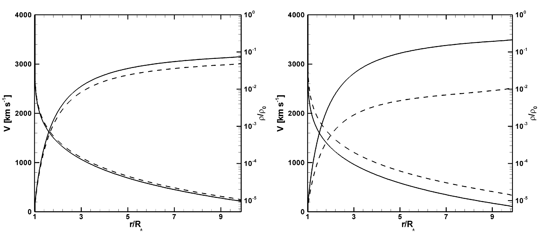
Figure 1: Left: The effect of continuum driving on a sub-Eddington, line-driven wind for $\,{\Gamma_{e}}=0.1$. The solid lines depict the wind parameters for the CAK force only, the dashed lines show the joint effect of both CAK line driving and continuum scattering. Clearly, the influence of the continuum term is negligeable. Right: The same variables , but for $\,{\Gamma_{e}}=0.5$. Here the difference caused by continuum driving is significantly more pronounced.

2 Sub-Eddington limit

As long as a star does not exceed the Eddington limit, continuum interaction alone cannot drive a stellar wind. However, it does influence the parameters of a (primarily) line-driven wind. Figure 1 demonstrates the influence of continuum driving on the stellar wind parameters. For these simulations we use the CAK line driving formalism described in ud-Doula & Owocki (2002), including both the finite disk correction factor and the modified gravity scaling of the line force (eq. [19] of OGS04 ). For the same stellar parameters ($50~{}\,{\rm M}_{\odot}$, $25~{}\,{\rm R}_{\odot}$, 50 000 K) and CAK parameters (${\bar{Q}=2.0\times 10^{3}}$, ${\alpha=2/3}$) but two different Eddington parameters ($\,{\Gamma_{e}}=L_{\star}/L_{\rm Edd}=0.1$ and 0.5,) we simulate the stellar wind with and without the continuum driving term.

Note that unlike the purely continuum-driven winds in the next section, these simulations do not contain any porosity effect. Namely, the continuum driving term in the equation of motion is simply:

$$g_{\rm cont}~{}=~{}\kappa_{e}\frac{F_{\rm rad}}{c},$$ (1)

with the continuum opacity $\kappa_{e}$ set to $0.3$ g/cm². These parameters give us an Eddington luminosity of ${L_{\rm Edd}=4\pi GcM/\kappa_{e}=8.33\times 10^{39}}$ erg/s. Figure 1 shows both the density (relative to the density at the stellar surface) and wind velocity as a function of radius for these two simulations. Clearly, for a low Eddington factor, the effect of continuum interaction on the wind parameters is negligeable. However, once the star approaches the Eddington limit, continuum driving increases the mass loss rate and decreases the terminal velocity. For $\,{\Gamma_{e}}=0.1$ the mass loss rate increases from $1.80\times 10^{-6}\,{{\rm M}_{\odot}~{}{\rm yr}^{-1}}$ to $1.92\times 10^{-6}\,{{\rm M}_{\odot}~{}{\rm yr}^{-1}}$ because of continuum driving. For $\,{\Gamma_{e}}=0.5$, these numbers are $2.18\times 10^{-6}\,{{\rm M}_{\odot}~{}{\rm yr}^{-1}}$ and $3.22\times 10^{-6}\,{{\rm M}_{\odot}~{}{\rm yr}^{-1}}$ respectively.

3 Analytical approximation

3.1 Wind velocity

For a radiatively driven outflow from a stellar surface, irrespective of the specific driving mechanism involved, the equation of motion can be written as

$$\biggl{[}1-\frac{a^{2}}{v^{2}}\biggr{]}v\frac{dv}{dr}~{}=~{}-\frac{GM_{\star}}{r^{2}}+\,{g_{\rm rad}}+\frac{2a^{2}}{r}-\frac{{\rm d}a^{2}}{{\rm d}r},$$ (2)

with $a$ the isothermal sound speed, $\,{g_{\rm rad}}$ the radiative acceleration and ${GM_{\star}}/{r^{2}}$ the inward gravitational acceleration. The last two terms on the right hand side are the result of the gas pressure gradient. In most cases they be neglected as their contribution to the velocity is usually negligeable next to the gravitational and radiative acceleration terms (OGS04, ). This assumption becomes incorrect only in those situations where the terminal velocity of the wind is close to the sound speed. If we neglect these gas pressure terms, we can rewrite equation (2) in a dimensionless form,

$$\biggl{[}1-\frac{w_{s}}{w}\biggr{]}w^{\prime}~{}=~{}-1+\,{\Gamma_{e}},$$ (3)

with $w=(v/\,{v_{\rm esc}})^{2}$, $w_{s}=(a/\,{v_{\rm esc}})^{2}$ and $\,{\Gamma_{e}}=\,{g_{\rm rad}}r^{2}/GM_{\star}$. Note that $\,{v_{\rm esc}}$ is defined as the escape velocity at the surface of the star $R_{\star}$ rather than as a local escape velocity. The gravitationally scaled inertial acceleration,

$$w^{\prime}~{}=~{}\frac{r^{2}v{\rm d}v/{\rm d}r}{GM_{\star}},$$ (4)

can be written in terms of the inverse radius coordinate $x\equiv 1-R_{\star}/r$, so that $w^{\prime}={\rm d}w/{\rm d}x$. This inverse radius coordinate makes for a more practical coordinate system than the radius itself, since it scales with the gravitational potential.

Since the escape velocity of a massive star is typically at least an order of magnitude larger than the local isothermal sound speed, we can in many cases neglect the bracketed term. For the porous atmosphere, OGS04 introduced a dimensionless parameter $k_{b}=\kappa_{\rm eff}/\kappa$, which gives the effective opacity of the local clumped medium vs. the opacity of the medium if it were completely homogeneous. Like OGS04 , we assume that the distribution $(f)$ of optical depths of the individual clumps can be described by a truncated power law,

$$\tau\frac{{\rm d}f}{{\rm d}\tau}~{}=~{}\frac{1}{\Gamma(\alpha_{p})}\biggl{(}\frac{\tau}{\tau_{0}}\biggr{)}^{\alpha_{p}}e^{-\tau/\tau_{0}},$$ (5)

with $\alpha_{p}\geq 0$ being the power-index and $\tau_{0}$ the optical depth of the thickest clump. Here $\Gamma(\alpha_{p})$ is the gamma function, rather than the Eddington parameter. This gives us:

$$k_{b}~{}=~{}\frac{(1+\tau_{0})^{1-\alpha_{p}}-1}{(1-\alpha_{p})\tau_{0}}.$$ (6)

For the full derivation see OGS04 .

As long as the clump characteristics are fixed, the optical depth $\tau_{0}$ scales with the density as,

$$\tau_{0}=\rho/\rho_{0},$$ (7)

where $\rho_{0}$ is the critical density at which the thickest blob has unit optical depth. This is calculated by

$$\rho_{0}~{}=~{}\frac{1}{\kappa h_{0}},$$ (8)

with $\kappa$ the continuum opacity and $h_{0}$ the porosity length of the thickest clump; the porosity length $h$ is defined as $L^{3}/l^{2}$, with $L$ being the typical separation between clumps and $l$ the size of the clump.

We thus rewrite eq. (3) by substituting,

$$\,{\Gamma_{e}}\longrightarrow\,{\Gamma_{e}}k_{b}(\tau_{0}),$$ (9)

for the Eddington parameter $\,{\Gamma_{e}}=L_{\star}/L_{\rm Edd}$. The scaled velocity gradient thus takes the form,

$$w^{\prime}(x)~{}=~{}\frac{\,{\Gamma_{e}}k_{b}[\tau_{0}(x)]-1}{1-w_{s}/w}\,.$$ (10)

This is a first-order differential equation that can be integrated using standard numerical techniques, starting from the sonic-point initial condition $w(x=0)=w_{s}$, where the vanishing of both the numerator and denominator on the right-hand side requires application of L’Hopital’s rule to evaluate the initial gradient,

$$w^{\prime}_{s}\equiv w^{\prime}(x=0)=\frac{\alpha_{p}}{4}\,\left[1+\sqrt{1+32w_{s}/\alpha_{p}}\right]\,.$$ (11)

By introducing the porosity term into the equation of motion, we have made the radiative acceleration dependent on the density and therefore on the radius. Under these circumstances, the radiative acceleration is only able to drive matter away from the star in the outermost layers of the star, producing a steady wind that can last as long as the star remains about the Eddington limit. In effect, porosity regulates the mass loss to a level that can be sustained in a nearly steady way throughout an LBV outburst. Here again the word “outburst” has to be interpreted in context. LBV outbursts can last years, which, though short compared to stellar evolutionary time, is quite long compared to a SN explosion. Most importantly, this is much longer than a typically dynamical flow time (ca. a free fall time, $R/\,{v_{\rm esc}}$, or a wind expansion time, $R/v_{\infty}$). As such, the mass loss can be well modeled in terms of steady-state wind solutions that assume the luminosity, etc. are constant over such dynamical timescales.

3.2 Mass loss rate

The mass loss rate induced by continuum driving is directly related to the luminosity of the star and the power index $\alpha_{p}$. The generic mass loss rate that follows from the porosity is

$$\dot{M}~{}=~{}\biggl{(}\frac{\rho_{\star}}{\rho_{0}}\biggr{)}\biggl{(}\frac{H}{h_{0}}\biggr{)}\frac{L_{\rm Edd}}{ac},$$ (12)

with $H$ the gravitational scale height of the gas at the sonic point. The sonic point density, $\rho_{\star}$, can be found through condition

$$\,{\Gamma_{e}}k_{b}~{}=~{}1.$$ (13)

For the simple case $\alpha_{p}=1/2$, this has the explicit solution

$$\biggl{(}\frac{\rho_{\star}}{\rho_{0}}\biggr{)}=4\,{\Gamma_{e}}\,(\,{\Gamma_{e}}-1)~{}~{}~{};~{}~{}~{}\alpha_{p}=\frac{1}{2}$$ (14)

which leads to an explicit expression for the mass loss rate (cf. eqn. (77) in OGS04 ),

$$\dot{M}=4(\,{\Gamma_{e}}-1)\frac{L_{\star}}{\eta_{0}ac}~{}~{}~{};~{}~{}~{}\alpha_{p}=\frac{1}{2}\,,$$ (15)

with ${\eta_{0}\equiv h_{0}/H}$. For more general cases, OGS04 also give explicit approximations for the expected mass loss rate, but in quoting values for this “analytic porosity model” below, we choose the more accurate approach of solving eqn. (13) implicitly, and using the resulting $\rho_{\star}$ to compute the associated mass loss rate from eq. (12).

4 Numerical method

For our numerical simulations we use the ZEUS hydrodynamics code (Stone & Norman, 1992; Clark, 1996). We do our computations on a 1D spherical grid with an inflow boundary in the center and outflow at the outer boundary. Continuum driving is modeled through an acceleration term $\,{\Gamma_{e}}k_{b}\,{g_{\rm grav}}$ added to the radial component of the equation of motion (see also, van Marle et al. (2008a)).

We start our simulation by initializing a 1D radial grid with matter moving away from the origin with a power law velocity distribution. At the inner boundary, we specify an inflow density, higher than the critical density $\rho_{s}$ to ensure that the sonic point (where the wind velocity equals the isothermal sound speed) is inside the grid. This inflow density remains constant during the simulation. The inflow velocity is time-dependent, and recalculated at each timestep such that the velocity gradient over the boundary is equal to the velocity gradient immediately above the boundary radius. Such “floating” boundary conditions allow approach to a stable, steady, flow solution, and have been successfully used for line-driven-wind simulations in both one (Owocki, Castor & Rybicki, 1988) and two dimensions (Owocki, Cranmer & Blondin, 1994).

The radial grid is not evenly spaced, but rather chosen in such a fashion that the individual grid size at the sonic point is always smaller than the local scale height.

For our simulations we assume that the gas is isothermal with a temperature of 50 000 K, which implies an isothermal sound speed of approximately $20~{}\,{\rm km~{}s^{-1}}$. The opacity of the gas is set to 0.4 gr/cm² (Thompson scattering opacity for pure hydrogen) and $\eta_{0}$ to 1. The radius and mass of the central star are set to 50 $\,{\rm R}_{\odot}$ and 50 $\,{\rm M}_{\odot}$ respectively. A star such as this has an Eddington luminosity of $6.24\times 10^{39}$ erg/s.

The grid extends from the stellar surface to a distance of ten times the stellar radius.

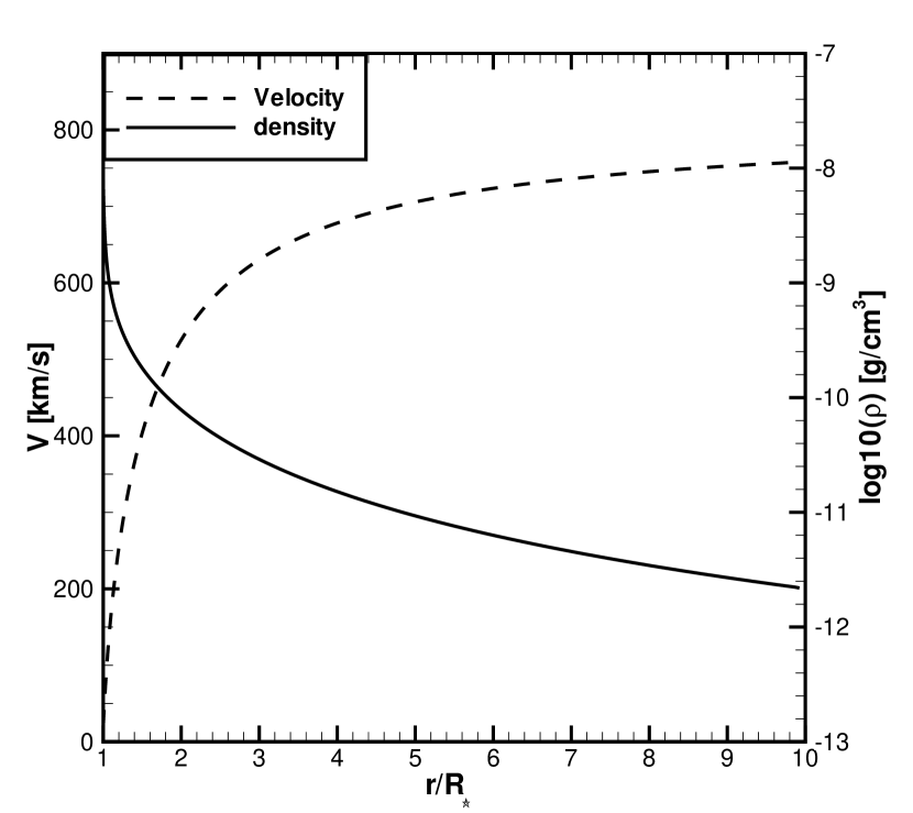
Figure 2: Wind velocity and density as a function of radius for a continuum-driven wind. On the horizontal axis, the local radius divided by the sonic point radius. Independent parameters: $\,{\Gamma_{e}}=3$, $\alpha_{p}=0.5$, $w_{\star}=0.001$

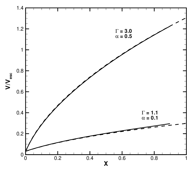
Figure 3: Wind velocity in units of the sonic point escape radius plotted versus the dimensionless radial coordinate $x=1-R_{sonic}/r$, comparing results for the analytical solution (dashed curves) and numerical simulation (solid curves) for a continuum-driven wind. The upper curves show results for the same parameters as figure 2, with $\,{\Gamma_{e}}=3$ and $\alpha_{p}=0.5$, while the lower curves are for the marginal super-Eddington case $\,{\Gamma_{e}}=1.1$, with $\alpha_{p}=0.1$. The agreement between numerical and analytical solutions is quite good, with only a slightly stronger differences for the $\,{\Gamma_{e}}=1.1$ case.

5 Results

A grid of 30 models was calculated, encompassing a parameter space of $0.1\leq\alpha_{p}\leq 0.8$ and $1.1\leq\,{\Gamma_{e}}\leq 6.0$. Stellar mass, radius surface temperature, opacity and clumping parameter $\eta_{0}$ were kept constant. A typical result for these calculations is shown in figure 2, which shows the density and wind velocity as a function of distance from the star.

$\,{\Gamma_{e}}$	$\alpha_{p}$	$\dot{M}_{an}$	$\dot{M}_{num}$	$\dot{M}_{an}/\dot{M}_{num}$	v/$\,{v_{\rm esc}}$
		$\,{\rm M}_{\odot}yr^{-1}$	$\,{\rm M}_{\odot}yr^{-1}$
6.0	0.8	4.86$\times 10^{-2}$	4.87$\times 10^{-2}$	0.997	1.93
6.0	0.5	1.98$\times 10^{-1}$	1.99$\times 10^{-1}$	0.997	1.80
6.0	0.3	2.09	2.10	0.994	1.50
6.0	0.2	3.92$\times 10^{1}$	3.99$\times 10^{1}$	0.982	1.13
6.0	0.1	2.87$\times 10^{5}$	3.00$\times 10^{5}$	0.956	0.655
4.0	0.8	2.43$\times 10^{-2}$	2.44$\times 10^{-2}$	0.995	1.53
4.0	0.5	7.94$\times 10^{-2}$	7.97$\times 10^{-2}$	0.996	1.47
4.0	0.3	5.23$\times 10^{-1}$	5.28$\times 10^{-1}$	0.991	1.31
4.0	0.2	5.13	5.23	0.981	1.08
4.0	0.1	4.97$\times 10^{3}$	5.21$\times 10^{3}$	0.954	0.655
3.0	0.8	1.42$\times 10^{-2}$	1.42$\times 10^{-2}$	0.997	1.26
3.0	0.5	3.97$\times 10^{-2}$	4.00$\times 10^{-2}$	0.992	1.23
3.0	0.3	1.91$\times 10^{-1}$	1.93$\times 10^{-1}$	0.990	1.14
3.0	0.2	1.20	1.22	0.985	1.00
3.0	0.1	2.80$\times 10^{2}$	2.92$\times 10^{2}$	0.959	0.654
2.0	0.8	5.83$\times 10^{-3}$	5.92$\times 10^{-3}$	0.984	0.907
2.0	0.5	1.32$\times 10^{-2}$	1.34$\times 10^{-2}$	0.987	0.894
2.0	0.3	4.20$\times 10^{-2}$	4.27$\times 10^{-2}$	0.983	0.862
2.0	0.2	1.47$\times 10^{-1}$	1.50$\times 10^{-1}$	0.980	0.812
2.0	0.1	4.83	5.06	0.955	0.633
1.5	0.8	2.53$\times 10^{-3}$	2.57$\times 10^{-3}$	0.984	0.643
1.5	0.5	4.96$\times 10^{-3}$	5.09$\times 10^{-3}$	0.974	0.643
1.5	0.3	1.19$\times 10^{-2}$	1.22$\times 10^{-2}$	0.978	0.632
1.5	0.2	2.87$\times 10^{-2}$	2.95$\times 10^{-2}$	0.973	0.616
1.5	0.1	2.61$\times 10^{-1}$	2.72$\times 10^{-1}$	0.958	0.551
1.1	0.8	4.33$\times 10^{-4}$	4.88$\times 10^{-4}$	0.888	0.301
1.1	0.5	7.27$\times 10^{-4}$	8.10$\times 10^{-4}$	0.898	0.300
1.1	0.3	1.32$\times 10^{-3}$	1.48$\times 10^{-3}$	0.892	0.299
1.1	0.2	2.20$\times 10^{-3}$	2.47$\times 10^{-3}$	0.891	0.298
1.1	0.1	6.08$\times 10^{-3}$	6.81$\times 10^{-3}$	0.892	0.293

Table 1: For parameters $\,{\Gamma_{e}}$ and $\alpha_{p}$ given in the first two columns, comparison of the mass loss rates predicted by the analytic porosity model (column 3) vs. those obtained in full numerical simulations (column 4), with the fifth column giving the ratio, analytical/numerical. The agreement is remarkably good, but with modest, ca. 10% differences for lower $\alpha_{p}$ or $\,{\Gamma_{e}}$ near unity. The last column gives the ratio between the terminal velocity and the escape speed from the sonic radius for the numerical models.

Table 1 compares mass loss rates for the numerical and analytical solutions for a sample of model parameters $\,{\Gamma_{e}}$ and $\alpha_{p}$. As noted above, the analytical mass loss rate is computed from eqn. (12) using the sonic point density derived from implicit solution of eqn. (13). The comparison shows that the analytical and numerical results coincide very well, with maximum differences of about 10% for $\,{\Gamma_{e}}$ near unity and small $\alpha_{p}$.

The wind velocity can be approximated semi-analytically by integrating equation (10). The results again match the numerical simulation quite well, as plotted in figure 3.

The match is partcularly good for the standard parameter set used in figure 2, with $\,{\Gamma_{e}}=3$ and $\alpha_{p}=0.5$. For the marginal super-Eddington model $\,{\Gamma_{e}}=1.1$ with small power index $\alpha_{p}=0.1$, which represents an almost pathogical case, the differences are greater, but still quite modest.

The complete results of the parameter study are shown in fig. 4, which shows the mass loss rate and terminal wind velocity for all simulations. As expected, the mass loss rate increases with $\,{\Gamma_{e}}$ and decreases with $\alpha_{p}$ as predicted in § 3. The terminal wind velocity increases both with $\,{\Gamma_{e}}$ and with $\alpha_{p}$. This is hardly surprising. A high $\,{\Gamma_{e}}$ means a strong radiative acceleration, which will lead to a higher velocity. A high $\alpha_{p}$ means a weaker coupling between matter and radiation. This decreases the mass loss rate, which for a given total available energy means an increase in velocity.

Mass loss rates in general are very high, though one should remember that photon-tiring was not included in these simulations. Although photon tiring does not change the mass loss rate at the stellar surface, it can prevent that part of the mass escapes the stellar gravity. Wind velocities are usually on the order of the escape velocity.

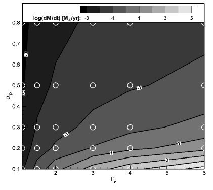
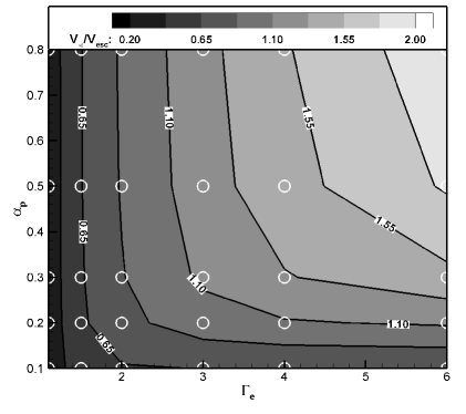
Figure 4: Left: Total mass loss rate in solar masses per year as a function of $\,{\Gamma_{e}}$ and $\alpha_{p}$. As predicted in the analytical approximations (see §3) the mass loss rate increases with $\,{\Gamma_{e}}$ but decreases with $\alpha_{p}$. Right: Terminal wind velocity divided by escape velocity as a function of $\,{\Gamma_{e}}$ and $\alpha_{p}$. The wind velocity increases with both $\,{\Gamma_{e}}$ and $\alpha_{p}$. The white circles indicate the actual datapoints, taken from table 1.

6 Photon tiring

One of the most interesting aspects of continuum-driven winds is their high mass loss rates, which gives rise to the phenomenon of “photon tired winds” suggested by Owocki & Gayley (1997). That is, winds in which the energy required to drive the gas out of the gravitational well is comparable or even larger than the energy available in the radiation field. In §6.1 we briefly cover the analytical description of these winds, and then continue with a numerical study of the case in which there is sufficient energy in the radiation field. The opposite limit, which gives rise to non-stationary solutions will be dealt in the subsequent publication.

6.1 Analytical approximation

If the stellar wind is driven by radiation, conservation of energy limits the maximum mechanical luminosity of the star to the radiative luminosity. This effect is known as photon tiring and was not included in the simulations described in the previous section.

The maximum amount of mass that can be driven of by radiation is the mass loss rate for which the mechanical luminosity of the wind matches the radiative luminosity,

$$\frac{1}{2}\dot{M}\,{v_{\rm esc}}^{2}~{}\leq~{}L_{\rm tir}~{}=~{}L_{\star},$$ (16)

with $L_{\star}$ the radiative luminosity of the star. This sets the upper limit for the mass loss rate to,

$$\dot{M}_{\rm tir}~{}=~{}\frac{2L_{\star}}{\,{v_{\rm esc}}^{2}}.$$ (17)

Note that this is the same for both line driving and continuum driving, and is unrelated to the composition of the stellar atmosphere. It is a fundamental property of the star. From this limit we calculate the photon tiring number $m$,

$$m~{}=~{}\frac{\dot{M}}{\dot{M}_{\rm tir}}.$$ (18)

As long as ${m\ll 1}$, photon tiring has no significant influence on the wind properties, but when ${m\lesssim 1}$ the situation changes. The radiation field of the star becomes depleted as much of its energy is used to drive the matter, leaving less energy available to drive the outer layers of the wind. The mass loss rate at the surface remains the same since it is set by the local radiative acceleration, but the wind velocity will decrease.

This will also influence observations, since radiative energy that is used to drive the wind will no longer be part of the visible radiation output of the star. For stars with line-driven winds, this is hardly worth considering. Even a Wolf-Rayet star with a powerful wind loses only a few percent of its luminosity to the wind. For continuum-driven winds, the effect can become quite significant.

Should $m$ actually exceed unity, the radiation field loses all its energy. As a result, the matter that leaves the stellar surface will not be able to reach the escape velocity and start to fall back onto the star. This will make it impossible to obtain a steady state solution.

A analytic analysis of the photon tiring effect was done by OGS04 , predicting that while the mass loss rate would remain the same, the velocity of the wind would drop. The new equation for the wind velocity becomes:

$$w^{\prime}(x)~{}=~{}\frac{\kappa_{\rm eff}[\tau_{0}(x)]}{\kappa}\,{\Gamma_{e}}[1-m(w+x)]-1.$$ (19)

Note that $\,{\Gamma_{e}}$ is no longer a constant but decreases with the radius and the velocity. The photon tiring number can be found by combining equations (15) and (18). For the special case where $\alpha_{p}=1/2$ this implies that,

$$m~{}=~{}0.13\frac{\,{\Gamma_{e}}-1}{\eta_{0}a_{20}}\frac{M_{\star}}{\,{\rm M}_{\odot}}\frac{\,{\rm R}_{\odot}}{R_{\star}},$$ (20)

with $a_{20}$ the sound speed in units of $20~{}{\rm km/s}$. The implications of this equation are quite clear. The relative effect of photon tiring increases with $\,{\Gamma_{e}}$ and decreases with the porosity length. This is to be expected, as a larger $\,{\Gamma_{e}}$ means an increase in mass loss rate, and therefore an increase in the amount of energy necessary to lift the material. A larger $\eta_{0}$ means a decrease in coupling between radiation and matter, such that the effect of photon tiring diminishes. The same is true for an increase in $\alpha_{p}$, so we can expect the effect of photon tiring to diminish with higher $\alpha_{p}$.

6.2 Numerical method

We calculate the effect of photon tiring by calculating the work integral along the radial gridline and subtracting the result from the total luminosity of the star. This provides us with the luminosity available at each radial grid point, which can then be used to accelerate the wind during the next time step.

The work integral is given by:

$$W{} =~{}\int_{R\star}^{r}\dot{m}(r)\,{g_{\rm rad}}{\rm d}r,$$ (21)

$$=~{}4\pi\int_{R\star}^{r}\rho(r)r^{2}v(r)\,{g_{\rm rad}}{\rm d}r.$$

Therefore, the effective luminosity at a given radius equals:

$$L{} =~{}L_{\star}-W,$$ (22)

$$=~{}L_{\star}-4\pi\int_{R\star}^{r}\rho(r)r^{2}v(r)\,{g_{\rm rad}}{\rm d}r$$

(van Marle et al., 2008a). Using this value for the luminosity, rather than the stellar luminosity used in the simulations described in §5, a new set of simulations was made for the same range of $\,{\Gamma_{e}}$ values and $\alpha_{p}=0.5$. All other parameters were kept the same as in §5.

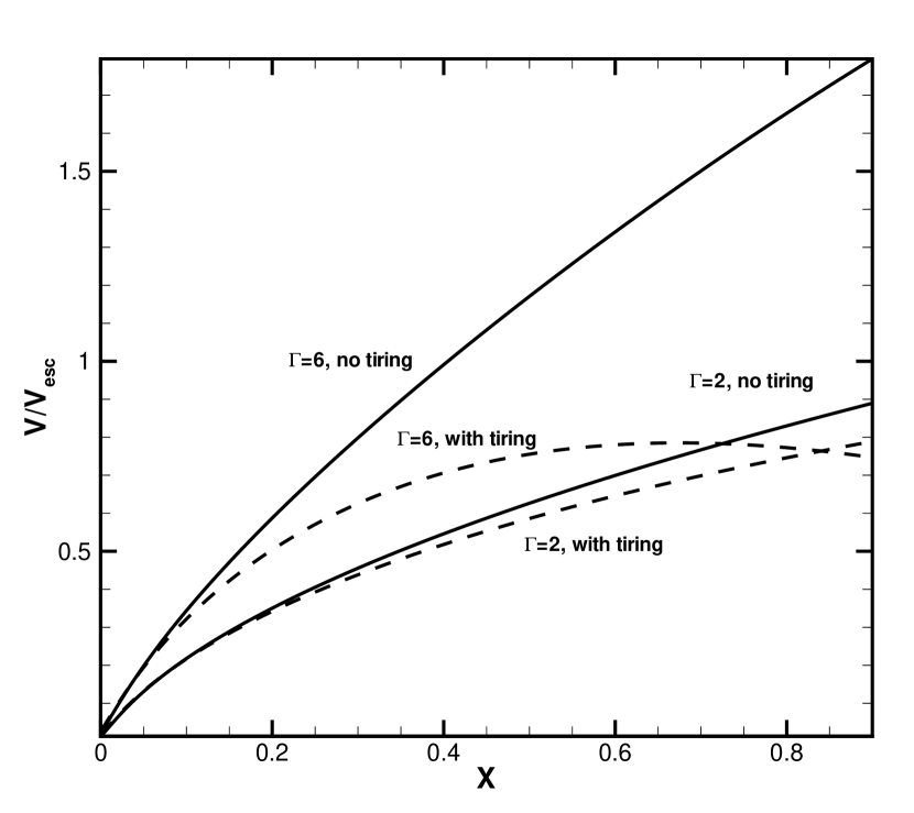
Figure 5: The effect of photon tiring on the wind velocity (I). Clearly, the effect is much larger for larger $\,{\Gamma_{e}}$.

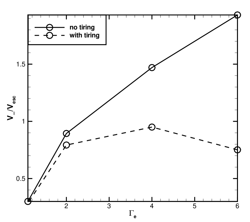
Figure 6: The effect of photon tiring on the wind velocity (II). This graph depicts the terminal velocity as a function of $\,{\Gamma_{e}}$ for simulations with and without photon tiring included. The effect clearly increases with $\,{\Gamma_{e}}$.

6.3 Numerical results

The effect of photon tiring is demonstrated in figure 5. For $\,{\Gamma_{e}}=2$, the effect is small, whereas for $\,{\Gamma_{e}}=6$ the effect is very large. Also, for the larger value of $\,{\Gamma_{e}}$, the velocity decreases beyond a certain radius. This corresponds to the radius where the luminosity falls below the Eddington luminosity. Note that the mass loss rate is independent of the tiring parameter and will therefore not change if photon tiring is included. This implies that the density of the wind increases, since the velocity decreases due to the photon tiring effect. It therefore also implies that the optical depth of the wind is higher as well.

In figure 6, one can see a comparison between the values of the terminal velocity obtained with and without photon tiring. The influence of photon tiring clearly increases with $\,{\Gamma_{e}}$. For large $\,{\Gamma_{e}}$, the terminal velocity itself actually decreases. It is clear from these results that for larger values of $\,{\Gamma_{e}}$ the photon tiring effect must be included in the numerical simulations, or the results will quickly become unphysical.

7 Discussion

A series of numerical simulations was carried out in order to test the analytical approximations for the porosity length formalism of continuum driving, published by OGS04 . The numerical results coincide well with the analytical results and demonstrate that this mechanism allows for powerful radiation-driven winds. This effect can explain the mass loss rates and wind velocities observed in Luminous Blue Variables such as $\eta$ Carinae.

The simulations also confirm that the photon tiring effect plays an important role in continuum driving as it places an upper limit on the mass loss rate. The effects of actually crossing the photon tiring limit have not yet been explored. This situation is much more complicated, since the simulations will no longer be able to reach a steady state solution. Ideally, such simulations should be done in two, or even three dimensions, to investigate the effect of interactions between different layers of the stellar wind as they move back and forth. Note that at this point we cannot predict how the star itself would react to such a situation. All our simulations have been done under the assumption that stellar parameters do not change significantly over time. It is possible that conditions in the outer layers of the star would change to reduce the driving force.

Porosity reduced continuum driving can also be important for the winds of other super-Eddington objects such as Novae (Shaviv, 2001b), accretion disks (Begelman, 2006) and transients like M85OT2006-1 (Kulkarni et al., 2007).

In a companion paper, (van Marle, Owocki & Shaviv, 2008b), we explore the situation where the star exceeds the photon tiring limit. We also intend eventually to generalize the simulations to multiple dimensions and explore the influence of stellar rotation on continuum-driven winds.

References

- Arons (1992) Arons, J., 1992, ApJ, 388, 561
- Begelman (2006) Begelman, M. C., 2002, ApJ, 643, 1065
- Clark (1996) Clark, D. A., 1996, ApJ, 457,291
- Davidson & Humphreys (1997) Davidson, K., & Humphreys, R. M., 1997, ARA&A, 35, 1
- Joss, Salpeter & Ostriker (1973) Joss, P., Salpeter, E., and Ostriker, J., 1973, ApJ, 181, 429
- Kulkarni et al. (2007) Kulkarni, S. et al., 2007, Nat, 447, 458
- Owocki, Castor & Rybicki (1988) Owocki, S. P., Castor, J. I. & Rybicki, G. B., 1988, ApJ, 335, 914
- Owocki, Cranmer & Blondin (1994) Owocki, S. P., Cranmer, S. R. & Blondin, J. M., 1994, ApJ, 424, 887
- Owocki & Gayley (1997) Owocki, S. P., & Gayley, K. G., 1997, Luminous Blue Variables: Massive Stars in Transition, 120, 121
- (10) Owocki, S. P., Gayley, K. G. & Shaviv, N. J., 2004, ApJ, 616, 525
- Owocki & van Marle (2008) Owocki, S. P. & van Marle, A. J., 2008, Conference proceedings, Massive Stars as Cosmic Engines, IAU Symp 250, ed. F. Bresolin, P. A. Crowther, & J. Puls, arXiv:0801.2519
- Shaviv (1998) Shaviv, N. J., 1998, ApJ, 494, L193
- Shaviv (2000) Shaviv, N. J., 2000, ApJ, 532, L137
- Shaviv (2001a) Shaviv, N. J., 2001a, ApJ, 549, 1093
- Shaviv (2001b) Shaviv, N. J., 2001b, MNRAS, 326, 126
- Smith (2002) Smith, N., 2002, MNRAS, 337, 1252
- Smith & Owocki (2006) Smith, N. & Owocki, S. P., 2006, ApJ, 645, L45
- Stone & Norman (1992) Stone, J. M. & Norman, M.L., 1992, ApJS, 80, 753
- ud-Doula & Owocki (2002) ud-Doula, A. & Owocki, S. P., 2002, ApJ, 576, 413
- van Marle et al. (2008a) van Marle, A. J., Owocki, S. P. & Shaviv, N. J., 2008a, proceedings of: First Stars III, Eds. B. O’Shea, T. Abel, A. Heger, AIPC, 990, 250
- van Marle, Owocki & Shaviv (2008b) van Marle, A. J., Owocki, S. P. & Shaviv, N. J., 2008, in preparation
- Vink & de Koter (2005) Vink, J. S. & de Koter, A., 2005, A&A, 442, 587