Analytical Tight-binding Approach for Ballistic Transport
through Armchair Graphene Ribbons:
Exact Solutions for Propagation through
Step-like and Barrier-like Potentials

Abstract

Based on a tight-binding approximation, we present analytical solutions for the wavefunction and propagation velocity of an electron in armchair graphene ribbons. The derived expressions are used for computing the transmission coefficients through step-like and barrier-like potentials. Our analytical solutions predict a new kind of transmission resonances for one-mode propagation in semiconducting ribbons. Contrary to the Klein paradox in graphene, this approach shows that backscattering for gapless mode is possible. In consistence with a higher order $\bf{k\cdot p}$ method, the backscattering probabilities vary with the square of the applied potential in the low-energy limit. We also demonstrate that gapless-mode propagation through a potential step in armchair ribbons can be described by the same through-step relation as that for an undimerized 1D chain of identical atoms.

I Introduction

Recently graphene sheet, a monolayer of covalent-bond carbon atoms forming a dense honeycomb crystal, has been obtained experimentally Geim and Novoselov (2007); Novoselov et al. (2004). Even at room temperature submicron graphene structures act as a high-mobility electron or hole conductors Geim and Novoselov (2007). This phenomenon has brought to life a promising field of carbon-based nanoelectronics, where graphene ribbons (GRs) could be used as connections in nanodevices.

The presence of armchair- and zigzag-shaped edges in graphene has strong implications for the spectrum of $\pi$-electrons Brey and Fertig (2006); Fujita et al. (1996); Nakada et al. (1996); Wakabayashi et al. (1999); Malysheva and Onipko (2008) and drastically changes the conducting properties of GRs. Especially, a zigzag edge provides localized edge states close to the Fermi level ($E_{F}=0$), which leads to the metallic type of conductivity. In contrast, any localized state does not appear in an armchair GR. An armchair GR can be easily made to be either metallic or semiconducting by controlling the width of the current channel.

Most of the intriguing electronic properties of GRs were first predicted by the tight-binding model Fujita et al. (1996); Nakada et al. (1996); Wakabayashi et al. (1999); Ezawa (2006); Robinson and Schomerus (2007); Schomerus (2007); Peres et al. (2006). These features are also well reproduced in the $\bf{k\cdot p}$ method Ando et al. (1998); Ando (2002) based on the decomposition of linear Schrödinger equations in the vicinity of zero-energy point. The commonly used $\bf{k\cdot p}$ equation is a two-dimensional analog of the relativistic Dirac equation Geim and Novoselov (2007); Brey and Fertig (2006); Ando (2002); Tworzydlo et al. (2006), which is a certain approximation of general tight-binding Schrödinger equations. The continuum Dirac description of the electronic states near $E=E_{F}$ has been shown to be quite accurate by comparing with a numerical solution in the nearest-neighbor tight-binding model Brey and Fertig (2006); Tworzydlo et al. (2006). Particularly, in the framework of the Dirac approach, perfect electron transmission is predicted through any high and wide potential barriers, known as the Klein paradox in graphene Katsnelson et al. (2006).

Recent analytical studies based on the relativistic Dirac equation have considered transmission through barriers Katsnelson et al. (2006), graphene wells Wakabayashi et al. (2007); Katsnelson (2006), double-barriers Pereira et al. (2007), quantum dots Silvestrov and Efetov (2007), superlattices Barbier et al. (2008), and $n-p$ junctions Cheianov and Fal’ko (2006). However, transport properties of these structures in the tight-binding model has not been analyzed systematically yet. Considerable attention has been paid to the effects of conductance quantization in GRs in the absence of scattering, where the quantization steps clearly indicate the number of propagating states crossing the Fermi level Peres et al. (2006).

In this paper, we develop an exact model of electron transport through armchair GRs based on the nearest-neighbor tight-binding approximation. (In contrast to the zigzag GRs, the armchair GR spectrum does not have a special band of edge states complicating the description.) We obtain simple analytical expressions for normalized wavefunctions and propagation velocity of an electron wave in armchair ribbons. No similar explicit solutions have been obtained for armchair GRs yet. In a tight-binding study by Zheng Zheng et al. (2007) of the electronic structure in armchair ribbons, the derived analytical form of wavefunction has not been used for describing charge transport in GRs.

On the basis of the analytical solutions for the wavefunction and propagation velocity of an electron in an infinite armchair GR, we describe the scattering problem through step-like and barrier-like profiles of site energy along the ribbon in closed form. Solving the corresponding equations for the scattering amplitudes, we obtain exact transmission coefficients in the atomistic (tight-binding) model analytically. For the energy region close to the Fermi level we compare our analytical expressions with their analogs obtained in the continuous (Dirac) model Katsnelson et al. (2006). Our general conclusion is that the validity of the relativistic approach based on the standard $\bf{k\cdot p}$ equation Ando (2002) is overestimated for the description of charge transport in armchair GRs. Specifically, for one-mode propagation in semimetal GRs, the deviation of transmission coefficients $T$ from the unity near the zero-energy point is proportional to the square of the step (barrier) magnitude, which contradicts the known Klein paradox in graphene Katsnelson et al. (2006). It is worth noting that similar deviations of transmission coefficients are intrinsic for the extended $\bf{k\cdot p}$ equation, based on higher order $\bf{k\cdot p}$ terms in the low-energy limit. Such high-order approximations lead to predicting small backscattering due to the effects of trigonal warping Ando et al. (1998) of the bands, destroying perfect transmission in the channel.

The paper is organized as follows. In the framework of the nearest-neighbor tight-binding formalism we calculate energy dispersion (Sec.II) and eigenstates (Sec. III) of electrons in the honeycomb graphene lattice. The lattice, in contrast to Ref. Zheng et al. (2007), is considered as a set of rectangular elementary cells of four nonequivalent atoms (Fig. 1). This assumption simplifies the description of electron transport processes in GRs in the presence of step-like or barrier-like site-energy profiles. Following Ref. Akhmerov and Beenakker (2008), in Section IV we derive boundary conditions for infinite GRs with armchair edges. By using a combination of early found eigenstates of the honeycomb lattice, we obtain normalized wave solutions for electrons in armchair GRs and formulate the quantization law for the transverse component $k^{m}$ of the wave vector. As a result, the full $\pi$-electron band spectra of graphene ribbon breaks into a set of subbands, whose features are discussed in Section V.

In Section VI, we find the group velocity and propagation direction of an electron in an armchair ribbon. It is shown that the group velocity is proportional to $\sin\theta$, where $\theta$ is the electron phase shift between two neighboring unit cells of the ribbon. In sections VII and VIII, the transmission probabilities through step-like and barrier-like potentials are calculated. Based on the exact solutions, in Section IX, we demonstrate that the transmission coefficients exhibit the new kind of resonance occurring when $\cos\theta=\cos\bar{\theta}$, where $\bar{\theta}$ is the inter-cell electron phase shift in the region where the potential exists. The number and positions of the transmission resonances are shown to be different in the regions $k^{m}<2\pi/3$ and $k^{m}>2\pi/3$. As for one-mode propagation in semimetal GRs ($k^{m}=2\pi/3$), our theory predicts no unit propagation. In Section X, by expanding the expressions for $\cos\theta$, $\cos\bar{\theta}$ in the vicinity of $E=0$, we explain why the Klein paradox does not hold in armchair GRs.

In Sec. XI, we discuss through-step and through-barrier probabilities and provide some examples. Conclusions are presented in Sec. XII. Appendices A (on electron flux in the tight-binding model) and B (on through-step transmission in a linear chain of identical atoms) describe some theoretical tools used in the paper. Appendix C contains some technical details related to obtaining our approximate solution from the Dirac solution Katsnelson et al. (2006).

II Dispersion relation for honeycomb graphene lattice

We consider the graphene honeycomb lattice as a set of rectangular elementary cells of four atoms $\alpha=l,\lambda,\rho,r$ (see Figure 1). By taking the tight-binding representation for molecular orbitals

$$|\Psi\rangle=\sum_{n,m=-\infty}^{\infty}\sum_{\alpha}\psi_{n,m,\alpha}|n,m,\alpha\rangle,$$

we come to the set of linear Schrödinger equations

$$\left\{\!\!\begin{array}[]{l}-E\psi_{n,m,l}=\psi_{n,m,\lambda}+\psi_{n,m+1,\lambda}+\psi_{n-1,m,r},\\ -E\psi_{n,m,\lambda}=\psi_{n,m,l}+\psi_{n,m,\rho}+\psi_{n,m-1,l},\\ -E\psi_{n,m,\rho}=\psi_{n,m,\lambda}+\psi_{n,m,r}+\psi_{n,m-1,r},\\ -E\psi_{n,m,r}=\psi_{n,m,\rho}+\psi_{n,m+1,\rho}+\psi_{n+1,m,l},\end{array}\right.$$ (1)

with respect to wave function components $\psi_{n,m,\alpha}=\langle\Psi|n,m,\alpha\rangle$. Here $|n,m,\alpha\rangle$ is $2{\rm p}_{z}$ orbital of $\alpha$-th atom in $\{n,m\}$-elementary cell, $E\equiv E/|\beta|$ is the electron energy in units of $|\beta|$, $\beta<0$ is a transfer integral between the nearest-neighbor carbon atoms. Site-energies of carbons equal zero and serve as a reference.

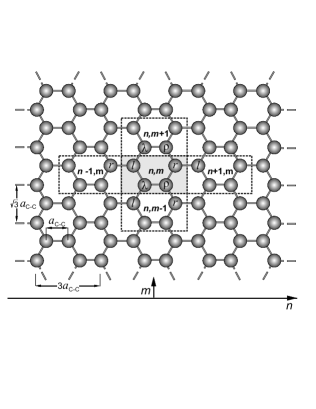
Figure 1: Sketch of 2D honeycomb lattice. The central shadowed block corresponds to an elementary cell $\{n,m\}$ consisting of 4 carbon atoms, labeled as $l,\lambda,\rho,r$. The lengths $3a_{\rm C-C}$ and $\sqrt{3}a_{\rm C-C}$ are the translation periods in $n$ and $m$ directions, $a_{\rm C-C}$ is ${\rm C-C}$ bond length.

We look for a solution of Eq. (1) in the form

$$\psi_{n,m,\alpha}=\phi_{\alpha}e^{ik^{n}n+ik^{m}m},\quad\alpha=l,\lambda,\rho,r,$$ (2)

where the dimensionless wave numbers $k^{n}(\equiv 3k_{x}a_{\rm C-C})$, $k^{m}(\equiv\sqrt{3}k_{y}a_{\rm C-C})$, and co-factors $\phi_{\alpha}$ are unknown coefficients, $k_{x}$ and $k_{y}$ are the components of the wave vector along $n$ and $m$ directions respectively. The lengths $3a_{\rm C-C}$ and $\sqrt{3}a_{\rm C-C}$ are the translation periods of the graphene sheet as depicted on the Fig. 1, where $a_{\rm C-C}$ is the C-C bond length.

Plugging in the solutions (2) into the system (1) gives the system of linear equations

$$\left\{\!\!\begin{array}[]{l}E\phi_{l}+\left(1+e^{ik^{m}}\right)\phi_{\lambda}+e^{-ik^{n}}\phi_{r}=0,\\ \left(1+e^{-ik^{m}}\right)\phi_{l}+E\phi_{\lambda}+\phi_{\rho}=0,\\ \phi_{\lambda}+E\phi_{\rho}+\left(1+e^{-ik^{m}}\right)\phi_{r}=0,\\ e^{ik^{n}}\phi_{l}+\left(1+e^{ik^{m}}\right)\phi_{\rho}+E\phi_{r}=0.\end{array}\right.$$ (3)

A nontrivial solution of Eq. (3) demands a zero determinant. It leads to the dispersion relation

$$\cos{k^{n}}=f(E,k^{m}),\qquad f(E,k^{m})=\frac{\left[E^{2}-1-4\cos^{2}\frac{k^{m}}{2}\right]^{2}}{8\cos^{2}\frac{k^{m}}{2}}-1,$$ (4)

defining the non-dimensional wave number $k^{n}$ in terms of $k^{m}$ and electron energy $E$. It follows from Eq.(4) that

$$E^{2}=1\pm 4\cos\frac{k^{m}}{2}\cos\frac{k^{n}}{2}+4\cos^{2}\frac{k^{m}}{2},$$ (5)

where index $\pm$ distinguishes two branches of the dispersion relation.

III Wave solution in graphene lattice

If the relation (4) holds, system (3) becomes degenerated, and we can express the coefficients $\phi_{l}$, $\phi_{\lambda}$, $\phi_{\rho}$ in terms of $\phi_{r}$, omitting the fourth equation in (3). The result can be written as follows

$$\phi_{\alpha}=C\,\widetilde{\phi}_{\alpha},\qquad\alpha=l,\lambda,\rho,r,$$ (6)

where

$$\widetilde{\phi}_{l}=-\frac{\left(E^{2}-1\right)e^{-ik^{n}}+4\cos^{2}\frac{k^{m}}{2}}{E\left(E^{2}-1-4\cos^{2}\frac{k^{m}}{2}\right)},\qquad\widetilde{\phi}_{\lambda}=\frac{\left(1+e^{-ik^{m}}\right)\left(1+e^{-ik^{n}}\right)}{E^{2}-1-4\cos^{2}\frac{k^{m}}{2}},$$

$$\widetilde{\phi}_{\rho}=-\frac{\left(1+e^{-ik^{m}}\right)\left(E^{2}+e^{-ik^{n}}-4\cos^{2}\frac{k^{m}}{2}\right)}{E\left(E^{2}-1-4\cos^{2}\frac{k^{m}}{2}\right)},\qquad\widetilde{\phi}_{r}=1.$$

Exploiting the energy dispersion relation (4), one can see that $|\widetilde{\phi}_{\alpha}|=1$ for the real-valued $k^{n}$. Introducing a new function

$$e^{i\theta}=-\frac{E^{2}-1+4e^{ik^{n}}\cos^{2}\frac{k^{m}}{2}}{E\left(E^{2}-1-4\cos^{2}\frac{k^{m}}{2}\right)}=-\frac{1\pm 2\cos\frac{k^{m}}{2}\,e^{ik^{n}/2}}{E},$$ (7)

we can get

$$\widetilde{\phi}_{l}=e^{i(\theta-k^{n})},\quad\widetilde{\phi}_{\lambda}=\pm e^{-i(k^{m}+k^{n})/2},\quad\widetilde{\phi}_{\rho}=\mp e^{-i(k^{m}+k^{n})/2+i\theta},\quad\widetilde{\phi}_{r}=1.$$ (8)

The choice of upper/lower signs in (7), (8) is determined by the sign in (5). Plugging in Eq. (8) into Eq. (6), and then the resulting expression into (2) gives the expressions for electron eigenstates in the honeycomb lattice

$$\psi_{n,m,\alpha}(k^{n},k^{m})=C\left\{\!\!\begin{array}[]{ll}e^{ik^{n}(n-1)+ik^{m}m+i\theta},&\alpha=l,\\ \pm e^{ik^{n}(n-1/2)+ik^{m}(m-1/2)},&\alpha=\lambda,\\ \mp e^{ik^{n}(n-1/2)+ik^{m}(m-1/2)+i\theta},&\alpha=\rho,\\ e^{ik^{n}n+ik^{m}m},&\alpha=r.\end{array}\right.$$ (9)

IV Wave solution for armchair GRs

Unlike the 2D honeycomb lattice, the electron wave function components $\psi_{n,m,\alpha}$ in GRs with armchair edges (see Figure 2) are the solution to the linear Schrödinger equations (1) only for inner elementary cells ($1<m\leq{\cal N}$). For boundary cells with $m=1$ or $m={\cal N}+1$, one needs to take into account that boundary carbons have only two neighbors (see Fig. 2).

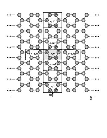
Figure 2: Sketch of infinite graphene ribbon with armchair edges. The solid-framed block is the unit cell $n$ of GR.

It demands the wave function to vanish on the set of absent sites Malysheva and Onipko (2008); Akhmerov and Beenakker (2008)^,

$$\psi_{n,0,l}=0,\quad\psi_{n,0,r}=0,\quad\psi_{n,{\cal N}+1,l}=0,\quad\psi_{n,{\cal N}+1,r}=0.$$ (10)

Similar boundary conditions were used in Refs Robinson and Schomerus (2007); Zheng et al. (2007).

To satisfy the relations (10), we represent the solution as a linear combination of the states (9),

$$\psi_{n,m,\alpha}(k^{n})=\psi_{n,m,\alpha}(k^{n},k^{m})-\psi_{n,m,\alpha}(k^{n},-k^{m}).$$

Since the definition (7) implies that $\theta(-k^{m})=\theta(k^{m})$, we finally obtain

$$\psi_{n,m,\alpha}(k^{n})=C^{\prime}\left\{\!\!\begin{array}[]{ll}e^{ik^{n}(n-1)+i\theta}\,\sin k^{m}m,&\alpha=l,\\ \pm e^{ik^{n}(n-1/2)}\,\sin k^{m}(m-1/2),&\alpha=\lambda,\\ \mp e^{ik^{n}(n-1/2)+i\theta}\,\sin k^{m}(m-1/2),&\alpha=\rho,\\ e^{ik^{n}n}\,\sin k^{m}m,&\alpha=r,\end{array}\right.$$ (11)

where

$$k^{m}\equiv k^{m}_{j}=\frac{\pi j}{{\cal N}+1},\qquad j=1,2,\ldots,{\cal N},$$ (12)

is the set of discretized transversal wave numbers, and the unknown constant $C^{\prime}(\equiv 2iC)$ can be found from the normalization condition over a unit cell of the armchair GR,

$$\sum_{m=1}^{{\cal N}}\left\{\left|\psi_{n,m,l}\right|^{2}+\left|\psi_{n,m,r}\right|^{2}\right\}+\sum_{m=1}^{{\cal N}+1}\left\{\left|\psi_{n,m,\lambda}\right|^{2}+\left|\psi_{n,m,\rho}\right|^{2}\right\}=1.$$

Then we finally get $C^{\prime}=[2({\cal N}+1)]^{-1/2}$.

V Band spectra of armchair GRs

Due to the transverse momentum quantization (12), the full $\pi$-electron band spectra of an armchair GR breaks into a set of subbands connected with each mode $j$ independently. Given $E$ and $k^{m}=k^{m}_{j}$, the dispersion relation (4) allows us to establish some important peculiarities of the $j$-th part of the band spectra. Following the theory of a one-dimensional crystal Onipko et al. (1997) with an arbitrary electronic structure of the elementary cell, each $j$-th band of graphene electron spectra includes 4 subbands, symmetrically disposed with respect to $E=0$. Real values of longitudinal wave number $k^{n}\in[0,\pi]$ define the region of propagating electron states (when $|f(E,k^{m}_{j})|<1$ in Eq.(4)). The cases $f(E,k^{m}_{j})>1$ and $f(E,k^{m}_{j})<-1$ are related to the complex values of $k^{m}=i\delta$ and $k^{m}=\pi+i\delta$, respectively. They refer to the forbidden zones – the gaps between neighboring electron subbands and the regions above the highest subband and below the lowest one. The subband boundaries correspond to $k^{m}=0$ or $k^{m}=\pi$ and satisfy the solutions to $f(E,k^{m}_{j})=1$ or $f(E,k^{m}_{j})=-1$, respectively. Since Eq.(4) defines only one $k^{m}$ for each energy level $E$, the subbands of the $j$th band cannot overlap, however, they may touch each other along the frontiers with the same $k^{m}(=0,\pi)$.

The results of the band spectrum modeling for armchair GRs with ${\cal N}=10-12$ are represented in Figure 3. Similar shapes are observed for GRs with arbitrary number ${\cal N}$.

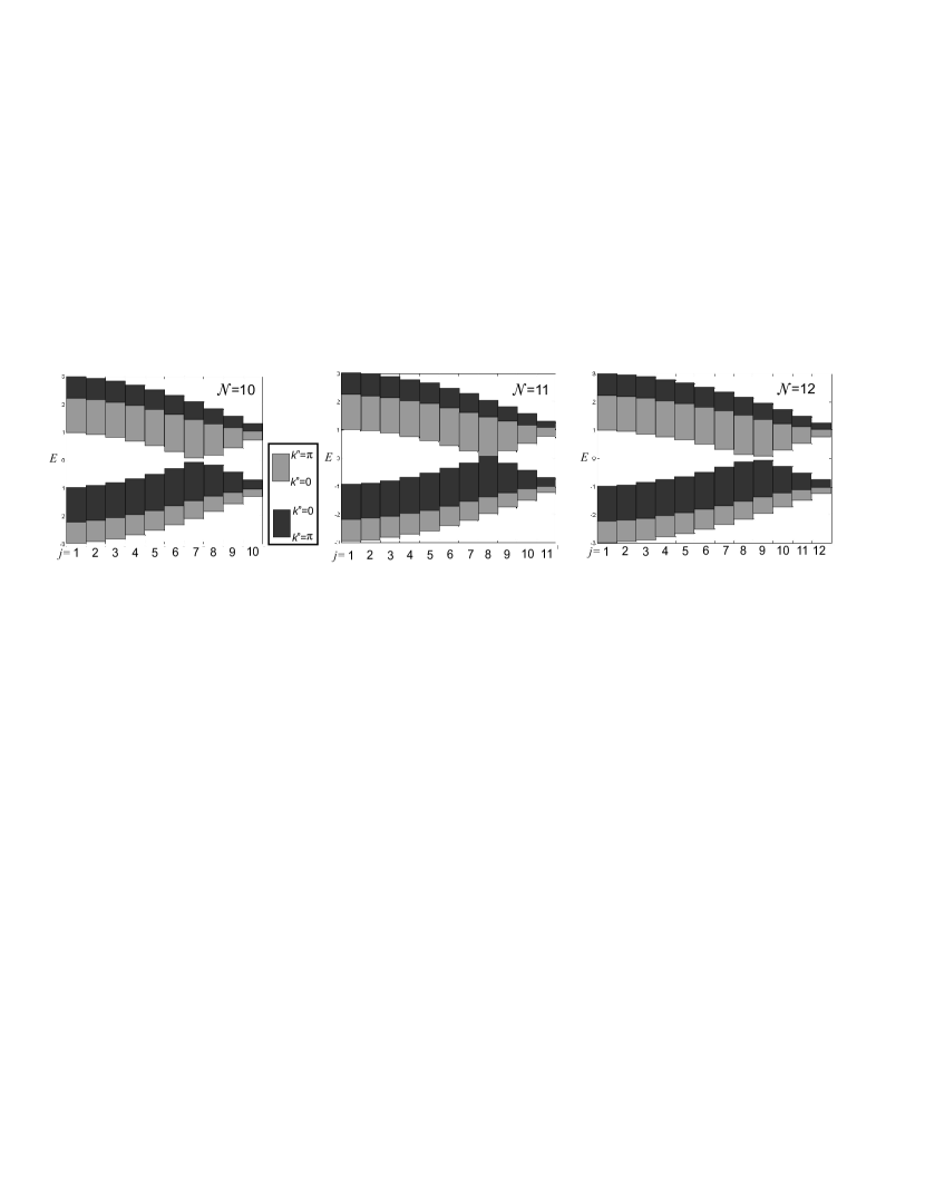
Figure 3: Examples of energy bands for armchair graphene ribbons with ${\cal N}=10-12$. The transverse momentum quantization results in subband series connected with each mode $j$ independently. Gray (black) rectangles mark subbands, whose bottom corresponds to $k^{n}=0$ ($k^{n}=\pi$) and whose top – to $k^{n}=\pi$ ($k^{n}=0$), as depicted in the framed panel. The border between black and gray rectangles in the positive- and negative-energy spectra determines the subband connecting $k^{n}=\pi$ frontiers, this is a degenerated solution to $f(E,k^{m}_{j})=-1$. The fundamental gap of a graphene ribbon is the minimal gap value $\Delta$ between the valence and conduction bands among all modes $j=1,\ldots,{\cal N}$.

The common features of the band spectra are: (I) bands are bounded by the energy interval $|E|\leq 3$; (II) the band structure is symmetric with respect to $E=0$; (III) if the number ${\cal N}+1$ is divisible by 3, the mode $j=2({\cal N}+1)/3$ (or $k^{m}_{j}=2\pi/3$) does not possess the energetic gap between positive- and negative-energy bands, and, therefore, it possesses the semimetal type of electron conductivity Brey and Fertig (2006); Malysheva and Onipko (2008); Robinson and Schomerus (2007); Zheng et al. (2007). For other $j$-modes there is a gap

$$\Delta=2\left|1-2\cos\frac{k^{m}}{2}\right|$$ (13)

between positive- and negative-energy subbands, which corresponds to a semiconducting ribbon whose gap decreases with increasing $\cal N$.

VI Propagation velocity

To obtain propagation velocity of the wave, we plug in the solution (11) into the relation (A2) for the electron flux $J$. Then $J=|\beta|\sin\theta/2\hbar$. Using the definition (7) and the first derivative of the dispersion relation (4) with respect to $E$, one can get

$$J=-\frac{|\beta|}{\hbar}\,\frac{2\sin k^{n}\cos^{2}\frac{k^{m}}{2}}{E\left(E^{2}-1-4\cos^{2}\frac{k^{m}}{2}\right)}=\frac{|\beta|}{\hbar}\,\frac{dE}{dk^{n}}.$$

Representing the flux $J$ as $(|\beta|/\hbar)v(k^{n})$, where $v(k^{n})$ is the dimensionless group velocity, we finally obtain

$$v(k^{n})=\frac{dE}{dk^{n}}=\frac{\sin\theta}{2}.$$ (14)

The sign of $v$ in Eq. (14) determines the moving direction of the propagating wave (11). For a subband $\left(=_{0}^{\pi}\right)$, whose bottom corresponds to $k^{n}=0$ and top to $k^{n}=\pi$ (see Fig. 3), the wave number $k^{n}$ increases along with $E$ ($dE/dk^{n}>0$). Therefore, $v>0$ and the state (11) describes the right-moving mode.

Similarly, in a subband of type $\left(=^{0}_{\pi}\right)$, we have $dE/dk^{n}<0$, and the wave solution (11) propagates to the left. Replacing $k^{n}$ with $-k^{n}$ in (7), (11), we obtain the expression describing a right-moving mode in these subbands

$$\psi_{n,m,\alpha}(-k^{n})=C^{\prime}\left\{\!\!\begin{array}[]{ll}e^{-ik^{n}(n-1)-i\theta}\,\sin k^{m}m,&\alpha=l,\\ \pm e^{-ik^{n}(n-1/2)}\,\sin k^{m}(m-1/2),&\alpha=\lambda,\\ \mp e^{-ik^{n}(n-1/2)-i\theta}\,\sin k^{m}(m-1/2),&\alpha=\rho,\\ e^{-ik^{n}n}\,\sin k^{m}m,&\alpha=r.\end{array}\right.$$ (15)

From (11) and (15), one can understand the physical meaning of the quantity $\theta$. Expressing $\psi_{n+1,m,l}(\pm k^{n})$ via $\psi_{n,m,r}(\pm k^{n})$, we get $\psi_{n+1,m,l}(\pm k^{n})=e^{\pm i\theta}\psi_{n,m,r}(\pm k^{n})$, i.e., an electron, propagating through the corresponding subbands, gains phase shift $\pm\theta$ between two neighboring unit cells of GR. The phase shift $\theta$ plays an important role in electron transmission through the ribbons, as discussed below. Also note that $\sin\theta>0$ inside the $\left(=_{0}^{\pi}\right)$-subbands and $\sin\theta<0$ in the subbands $\left(=^{0}_{\pi}\right)$, which is also seen from the relation (14).

The derived analytical form of the wavefunctions (11), (15) and the expression (14) for propagation velocity will be used below to investigate transport properties of armchair GRs in the presence of step-like or barrier-like potentials.

VII Transmission probability through a potential step

In this section, we derive the transmission coefficient for an electron with energy $E$, transverse and longitudinal wave numbers $k^{m}$, $k^{n}$, meeting the electrostatic potential

$$V(n)=\left\{\!\!\begin{array}[]{ll}0,&n\leq 0,\\ V_{0},&n\geq 1,\end{array}\right.$$

in an armchair ribbon. We denote the wavefunction by $\psi^{{}^{\rm left}}_{n,m,\alpha}$ for $n\leq 0$ and $\psi^{{}^{\rm right}}_{n,m,\alpha}$ for $n\geq 1$. Let $U_{0}\equiv eV_{0}/|\beta|$.

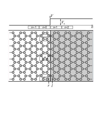
Figure 4: Sketch of a graphene ribbon with armchair edges modified by a step-like potential. Unit cells with $n\leq 0$ and $n\geq 1$ belong to the left and right leads of GR, respectively.

The Schrödinger equations for all atoms in both leads are used to obtain the probabilities of electron scattering through the potential step. The comparison of these equations near the interface between two regions ($n=0,1$) allows us to write down the matching conditions²⁶ as follows

$$\psi^{{}^{\rm left}}_{0,m,r}=\psi^{{}^{\rm right}}_{0,m,r},\quad\psi^{{}^{\rm left}}_{1,m,l}=\psi^{{}^{\rm right}}_{1,m,l},\qquad m=1,\ldots,{\cal N}.$$ (16)

Similar conditions for the tight-binding model were used in Ref. Schomerus (2007) and for the Dirac equation in Refs. Tworzydlo et al. (2006); Katsnelson et al. (2006); Katsnelson (2006).

Since the matching conditions (16) do not mix the modes, we need to sew only the $j$-th solutions in each region under study. Wave solutions, describing incident and reflected electron waves in the left lead, can be constructed from the states (11) and (15). For the right region, one needs to take into account the shift of site energies produced by the applied potential. Introducing additional notation for longitudinal wave number $\bar{k}^{n}$, phase $\bar{\theta}$ and group velocity $\bar{v}(\bar{k}^{n})$ in the right lead,

$$\bar{k}^{n}\equiv k^{n}(E\rightarrow E-U_{0}),\quad\bar{\theta}\equiv\theta(E\rightarrow E-U_{0},k^{n}\rightarrow\bar{k}^{n}),\quad\bar{v}(\bar{k}^{n})\equiv\frac{\sin\bar{\theta}}{2},$$ (17)

we first consider the case of propagation through the $\left(=_{0}^{\pi}\right)$-subbands in both regions, as depicted on the a-panel of Fig. 5.

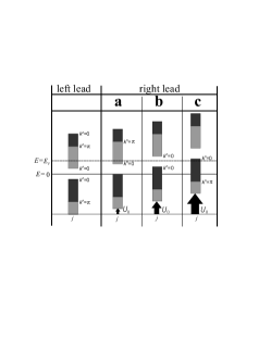
Figure 5: Three possible types of electron subband disposition in the right region. The Fermi level is assumed to be located in a $\left(=_{0}^{\pi}\right)$-subband of the left lead and incident wave is described by the solution (11). a) Electron propagates through a $\left(=_{0}^{\pi}\right)$-subband in the right region; b) the Fermi level belongs to the band-gap of the right lead, which results in total reflection; c) electron propagates through a $\left(=^{0}_{\pi}\right)$-subband in the right region. This case corresponds to the solution (15) for an outgoing wave in the lead.

The solutions describing the incident and reflected electron waves in the left lead and the outgoing wave in the right region should be taken in the following form

$$\psi^{{}^{\rm left}}_{n,m,l}=\left[e^{ik^{n}(n-1)+i\theta}+re^{-ik^{n}(n-1)-i\theta}\right]\sin k^{m}_{j}m,\quad\psi^{{}^{\rm left}}_{n,m,r}=\left[e^{ik^{n}n}+re^{-ik^{n}n}\right]\sin k^{m}_{j}m,$$ (18)

$$\psi^{{}^{\rm right}}_{n,m,l}=te^{i\bar{k}^{n}(n-1)+i\bar{\theta}}\sin k^{m}_{j}m,\quad\psi^{{}^{\rm right}}_{n,m,r}=te^{i\bar{k}^{n}n}\sin k^{m}_{j}m,$$ (19)

where $r$ and $t$ are the amplitudes of the reflected and transmitted waves excited by the incident wave with transverse mode $j$. (We omit the factor $C^{\prime}$ for simplicity.) After plugging in 18), (19) into the conditions (16), we get the following two equations

$$\left\{\!\!\begin{array}[]{l}1+r=t,\\ e^{i\theta}+re^{-i\theta}=te^{i\bar{\theta}}.\end{array}\right.$$

Their solution is

$$r=-\frac{e^{i\bar{\theta}}-e^{i\theta}}{e^{i\bar{\theta}}-e^{-i\theta}},\qquad t=\frac{2i\sin\theta}{e^{i\bar{\theta}}-e^{-i\theta}}.$$ (20)

The reflection and transmission probabilities $R$ and $T$ can be directly found from the scattering amplitudes $r,t$, using their definitions: $R=|r|^{2}$ and $T=|t|^{2}\bar{v}(\bar{k}^{n})/v(k^{n})=|t|^{2}\sin\bar{\theta}/\sin\theta$. In this way, we obtain the expression for an electron propagating via $\left(=_{0}^{\pi}\right)$-subbands in both leads

$$T=\frac{4\sin\theta\,\sin\bar{\theta}}{4\sin\theta\,\sin\bar{\theta}+\left(\sin\bar{\theta}-\sin\theta\right)^{2}+\left(\cos\bar{\theta}-\cos\theta\right)^{2}}.$$

The b-panel of Figure 5 corresponds to the case when the electron energy belongs to the forbidden band in the right region (it is impossible for one-mode propagation through a semimetal ribbon with a zero-gap, $k^{m}_{j}=2\pi/3$). In this case, the wave number $\bar{k}^{n}$ takes imaginary values, and the expression for $t$ in (20) is to be omitted. At the same time, for imaginary-valued $\bar{k}^{n}$ the expression for $e^{i\bar{\theta}}$ becomes real, which results in $R=1$ after using the $r$-solution from (20).

For an electron moving through a $\left(=^{0}_{\pi}\right)$-subband in the right lead, the c-panel of Figure 5, we use the solution (15) for an outgoing wave (see the definitions (17)). Thus, we obtain

$$T=\frac{-4\sin\theta\,\sin\bar{\theta}}{-4\sin\theta\,\sin\bar{\theta}+\left(\sin\bar{\theta}+\sin\theta\right)^{2}+\left(\cos\bar{\theta}-\cos\theta\right)^{2}},$$

where $\sin\bar{\theta}<0$, as stated in Sec.VI. In a similar way, one can determine the transmission coefficient for an electron propagating through arbitrary subbands in the left and right leads

$$T^{\rm step}=\frac{4|\sin\theta\,\sin\bar{\theta}|}{4|\sin\theta\,\sin\bar{\theta}|+\left(|\sin\bar{\theta}|-|\sin\theta|\right)^{2}+\left(\cos\bar{\theta}-\cos\theta\right)^{2}}.$$ (21)

The common relation (21) must be supplemented with the expressions for $\cos\theta$, $\cos\bar{\theta}$ determined from (7) and (17). Then, from the energy dispersion (4), we finally obtain

$$\cos\theta=g(E,k^{m}),\qquad\cos\bar{\theta}=g(E-U_{0},k^{m}),$$ (22)

where the function $g$ is described by the simple relation

$$g(E,k^{m})=-\frac{E^{2}+1-4\cos^{2}\frac{k^{m}}{2}}{2E}.$$ (23)

The analytical expression (21) with the definitions (22), (23) is one of the central points of this paper since it makes it possible to compute the transmission coefficient through a potential step without recourse to the initial dispersion relation (4).

It is worth noting how similar the solution (21) to the relation (B4) is, though the relation (B4) is for through-step transmission coefficient in the 1D undimerized chain of identical atoms. In other words, the inter-cell variables $\theta$, $\bar{\theta}$ for GRs act as wave numbers $k$, $\bar{k}$ in the linear chain model, whose unit cell degenerates to a zero-sized atom. We’ll return to this issue in Sec. IX.

VIII Transmission coefficient through a potential barrier

To obtain the exact expression for the electron transmission probability through a potential barrier

$$V(n)=\left\{\!\!\begin{array}[]{ll}0,&n\leq 0,\\ V_{0},&1\leq n\leq N,\\ 0,&n\geq N+1,\end{array}\right.$$

(see Fig. 6), we denote the wavefunction by $\psi^{{}^{\rm left}}_{n,m,\alpha}$ for the left lead ($n\leq 0$), $\psi^{{}^{\rm in}}_{n,m,\alpha}$ for the ”in” region ($1\leq n\leq N$) perturbed by the potential, $\psi^{{}^{\rm right}}_{n,m,\alpha}$ for the right lead ($n\geq N+1$), and keep the same notation for the disturbed region, as in the previous section.

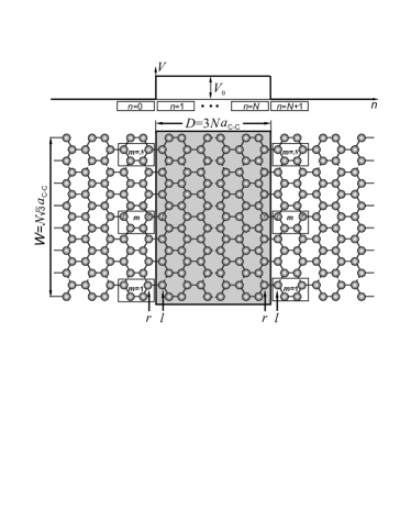
Figure 6: Sketch of a graphene ribbon with armchair edges modified by the barrier-like potential. $W$ and $D$ are the ribbon width and length of the disturbed region, respectively.

By analogy with the matching conditions (16), we need to have the following relations satisfied

$$\begin{array}[]{ll}\psi^{{}^{\rm left}}_{0,m,r}=\psi^{{}^{\rm in}}_{0,m,r},&\psi^{{}^{\rm left}}_{1,m,l}=\psi^{{}^{\rm in}}_{1,m,l},\\ \psi^{{}^{\rm in}}_{N,m,r}=\psi^{{}^{\rm right}}_{N,m,r},&\psi^{{}^{\rm in}}_{N+1,m,l}=\psi^{{}^{\rm right}}_{N+1,m,l}.\end{array}$$ (24)

As before, the solutions are determined using the states (11) and (15).

For an electron propagating through a $\left(=_{0}^{\pi}\right)$ subband in the left lead the wavefunction expressions are presented by (18). The outgoing wave in the right lead is constructed from the state (11),

$$\phi^{{\rm right}}_{n,m,\alpha}=t\sin(k^{m}_{j}m)\,\left\{\!\!\begin{array}[]{ll}e^{ik^{n}(n-1)+i\theta},&\alpha=l,\\ e^{ik^{n}n},&\alpha=r.\end{array}\right.$$

For the in-region we determine a solution

$$\psi^{{\rm in}}_{n,m,\alpha}=\sin(k^{m}_{j}m)\left\{\!\!\begin{array}[]{ll}\left(ae^{i\bar{k}^{n}(n-1)+i\bar{\theta}}+be^{-i\bar{k}^{n}(n-1)-i\bar{\theta}}\right),&\alpha=l,\\ \left(ae^{i\bar{k}^{n}n}+be^{-i\bar{k}^{n}n}\right),&\alpha=r,\end{array}\right.$$

where $a$ and $b$ are additional unknown constants. The solution does not depend on the subband type of propagation in the disturbed region. The case of tunneling through a gap, with $\bar{k}^{n}$ imaginary, is not considered in the paper.

Using the matching conditions (24), we obtain the following four equations with four unknowns $r$, $t$, $a$ and $b$

$$\left\{\begin{array}[]{l}a+b=1+r,\\ e^{i\theta}+re^{-i\theta}=ae^{i\bar{\theta}}+be^{-i\bar{\theta}},\\ t\,e^{ik^{n}N}=ae^{i\bar{k}^{n}N}+be^{-i\bar{k}^{n}N},\\ ae^{i\bar{k}^{n}N+i\bar{\theta}}+be^{-i\bar{k}^{n}N-i\bar{\theta}}=te^{ik^{n}N+i\theta}.\end{array}\right.$$ (26)

Solving (26) with respect to $t$, we obtain

$$t=-\frac{2ig_{\rm nd}\sin\theta}{\left(g_{\rm d}-e^{-i\theta}\right)^{2}-g^{2}_{\rm nd}}\,e^{-ik^{n}N-i\theta},$$

where the functions

$$g_{\rm d}=\frac{\sin\bar{k}^{n}N}{\sin(\bar{k}^{n}N+\bar{\theta})},\qquad g_{\rm nd}=\frac{\sin\bar{\theta}}{\sin(\bar{k}^{n}N+\bar{\theta})}$$ (27)

depend only on the ”disturbed” variables $\bar{k}^{n}$ and $\bar{\theta}$. Since, by definition, $T=|t|^{2}$, the through-barrier transmission probability can be written in the following compact form²⁶

$$T^{\rm bar}=\frac{\sin^{2}\theta\,\sin^{2}\bar{\theta}}{\sin^{2}\theta\sin^{2}\bar{\theta}+\left(\cos\theta-\cos\bar{\theta}\right)^{2}\sin^{2}(\bar{k}^{n}N)}.$$ (28)

It is easy to verify that the transmission coefficient (28) remains unchanged for propagation through a $\left(=^{0}_{\pi}\right)$-subband in external (left and right) leads.

As follows from Eq. (28), the unit transmission occurs under the coincidence of $\cos\theta$ and $\cos\bar{\theta}$. This can be viewed as a new type of resonance, which differs from the familiar resonance condition $\sin(\bar{k}^{n}N)=0$. Some of its properties are studied in the next section.

IX Unit propagation condition

The transmission coefficients (21) and (28) through step-like and barrier-like potentials exhibit the unit propagation at $\theta$s such that $\cos\theta=\cos\bar{\theta}$, which are the roots of the equation

$$g(E,k^{m})=g(E-U_{0},k^{m}),$$ (29)

(see the definitions (22)). Particularly, Eq.(29) has no solution for a function $g(E,k^{m})$ that is monotonic with respect to $E$, except when $U_{0}=0$, the usual condition of the unit transmission.

For the case of one-mode propagation in semimetal GRs ($k^{m}=2\pi/3$) the relation (23) reduces to the simple linear dependence

$$g(E,k^{m})=-E/2,$$ (30)

which corresponds to the absence of perfect transmission. In cases of one-mode propagation in semiconducting GRs ($k^{m}\neq 2\pi/3$), due to the oddness of $g$ with respect to $E$, we confine our attention to the properties of $g(E,k^{m})$ inside the positive-energy region $E>0$. Differentiating $g(E,k^{m})$ with respect to $E$,

$$\frac{dg(E,k^{m})}{dE}\equiv-\frac{1}{2}+\frac{1-4\cos^{2}\frac{k^{m}}{2}}{2E^{2}}=0,\qquad d^{2}g/dE^{2}>0,$$

one can compute the point where the function attains its minimum value

$$E=E_{min}(k^{m})=\sqrt{1-4\cos^{2}\frac{k^{m}}{2}},$$ (31)

only for transverse wave numbers in the region $2\pi/3<k^{m}\leq\pi$. For the case when $0<k^{m}<2\pi/3$, we obtain $dg/dE\neq 0$ and $d^{2}g/dE^{2}<0$. Hence $g(E,k^{m})$ is convex and monotone decreasing. Figure 7 presents the in-band behaviour of $g(E,k^{m})$ with respect to $E$ for the above mentioned $k^{m}$-domains: $k^{m}=2\pi/3-0.1(<2\pi/3)$, $k^{m}=2\pi/3$, and $k^{m}=2\pi/3+0.1(>2\pi/3)$.

As follows from the relation (29), the transmission probabilities (21) and (28) reach unity at the points where the curve $g(E,k^{m})$ crosses $g(E-U_{0},k^{m})$. Such intersections are possible even for $U_{0}\ll 1$ in the region $2\pi/3<k^{m}\leq\pi$ (see Figure 7), where the resonance occurs near the energy level (31). In the case when $0<k^{m}<2\pi/3$, unit propagation takes place if the value of $U_{0}$ exceeds the energy gap $\Delta$.

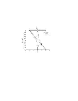
Figure 7: Behaviour of $g(E,k^{m})$ inside the positive- and negative-energy bands for $k^{m}=2\pi/3$ (solid line) and $k^{m}=2\pi/3\mp 0.1$. The shaded rectangles represent the band positions for the transverse wave number $k^{m}=2\pi/3-0.1$, where $\Delta$ is the energy gap for given $k^{m}$.

To show this, we plug in the relation (23) into Eq. (29) and get

$$E(E-U_{0})=x,\qquad x=1-4\cos^{2}\frac{k^{m}}{2}.$$ (32)

The unit transmission points are real-valued roots of the Eq. (32),

$$E^{\rm res}=U_{0}/2\pm\sqrt{(U_{0}/2)^{2}+x}.$$ (33)

In the interval $0<k^{m}<2\pi/3$, $x$ is negative, and the transmission resonances exist only if $|U_{0}|$ exceeds $2|x|^{1/2}$. Expressing $x$ in terms of the energy gap $\Delta$ (see Eq.(13)), we obtain the following inequality for transmission resonances in this region

$$|U_{0}|\geq 4\sqrt{\Delta(\Delta+1)}.$$ (34)

The energies of the transmission resonances versus $U_{0}$ are plotted in Figure 8. If $2\pi/3<k^{m}\leq\pi$, the indicated region $|U_{0}|\leq 1$ contains two resonances, one of which belongs to the valence band, and another to the conduction band. In the case when $0<k^{m}<2\pi/3$, two unit transmissions are observed if the condition (34) holds. The resonance positions depend on the sign of $U_{0}$. Both of them belong to the valence band if $U_{0}>0$ and to the conduction band if $U_{0}<0$.

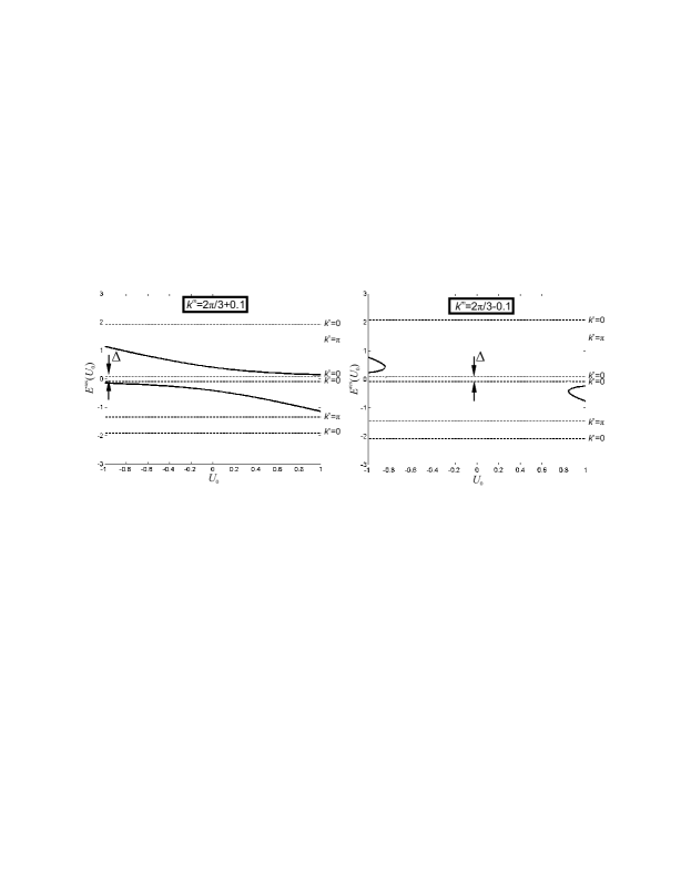
Figure 8: Resonance energies $E^{\rm res}$ (solid lines) versus $U_{0}$ for transverse wave numbers $k^{m}=2\pi/3\pm 0.1$. Dashed horizontal lines correspond to the boundaries of the positive- and negative energy subbands for the left region, where $\Delta$ is the energy gap for given $k^{m}$.

The case of one-mode propagation in semimetal ribbons ($k^{m}=2\pi/3$) deserves additional attention. The linear dependence of $g(E,k^{m})$ with respect to $E$ (given by Eq. (30)), makes unit propagation impossible. This shows that the Klein paradox Katsnelson et al. (2006) does not hold in armchair GRs. Specifically, plugging in (22) and (30) into (21) produces

$$T=\frac{4\sqrt{(4-E^{2})[4-(E-U_{0})^{2}]}}{\left(\sqrt{4-E^{2}}+\sqrt{4-(E-U_{0})^{2}}\right)^{2}+U_{0}^{2}},$$ (35)

which can be reduced to

$$T\approx 1-U_{0}^{2}/16$$ (36)

for $E=0$ and $|U_{0}|\ll 1$.

It is worth noting that the through-step expression (35) coincides with its analog for electron transmission through a potential step in an undimerized linear chain of identical atoms (see Appendix B). Specifically, the through-step coefficient (35) in the vicinity of the neutrality point $E=0$ is exactly the same as the transmission coefficient through a step potential formed in the linear chain when the electron energy is located near the corresponding band center.

X Low-energy limit

Most theoretical studies on the electronic properties of all-carbon honeycomb lattices are based on the $\bf{k\cdot p}$ approximation in the vicinity of the zero-energy point, leading to the two-dimensional analog of the relativistic Dirac equation Geim and Novoselov (2007); Ando (2002); Brey and Fertig (2006); Katsnelson et al. (2006). Rewriting the energy dispersion (5)

$$E^{2}=\left(1\pm 2\cos\frac{k^{m}}{2}\right)^{2}\mp 4\cos\frac{k^{m}}{2}\left(1-\cos\frac{k^{n}}{2}\right),$$

we see that in the low-energy limit only the branch

$$E^{2}=\left(1-2\cos\frac{k^{m}}{2}\right)^{2}+4\cos\frac{k^{m}}{2}\left(1-\cos\frac{k^{n}}{2}\right)$$ (37)

of the dispersion relation takes part in electron transport. In terms of the deviation of ${\mathbf{k}}=(k^{n},k^{m})$ from the zero-energy point $(0,2\pi/3)$,

$$k^{n}=3k_{x}a_{\rm C-C},\qquad k^{m}=2\pi/3+\sqrt{3}k_{y}a_{\rm C-C},$$

we can expand (37) into series $|k_{x(y)}|a_{\rm C-C}\ll 1$ up to and including the quadratic terms. Then

$$E(k_{x},k_{y})=\pm\frac{3a_{\rm C-C}}{2}\sqrt{k_{x}^{2}+k_{y}^{2}},$$ (38)

which is similar to the cone-like form of electron dispersion Geim and Novoselov (2007); Ando (2002); Malysheva and Onipko (2008). In the same way, the formula (7) for inter-cell electron phase shift $\theta$ reduces to

$$e^{i\theta}=-\frac{1-2\cos\frac{k^{m}}{2}\,e^{ik^{n}/2}}{E}=i\,{\rm sgn}(E)\,\frac{k_{x}+ik_{y}}{\sqrt{k_{x}^{2}+k_{y}^{2}}}+O(k_{x},k_{y})+\ldots\,,$$ (39)

where

$$O(k_{x},k_{y})=-\frac{a_{\rm C-C}}{4}\,{\rm sgn}(E)\,\frac{3k_{x}^{2}+6ik_{x}k_{y}+k_{y}^{2}}{\sqrt{k_{x}^{2}+k_{y}^{2}}}.$$ (40)

Retaining only the first term in Eq. (39), we come to

$$e^{i\theta}=i\,{\rm sgn}(E)\,e^{i\phi},\qquad\phi=\tan^{-1}\frac{k_{y}}{k_{x}},$$ (41)

where $\phi$ is the known phase factor from low-energy theory Katsnelson et al. (2006); Katsnelson (2006). Expressing the transmission coefficients (21) and (28) in terms of $\phi$, $\bar{\phi}\equiv\phi(k_{x}\rightarrow\bar{k}_{x})$, we obtain the following approximate expressions

$$T^{\rm step}_{\rm appr}=\frac{4|\cos\phi\,\cos\bar{\phi}|}{\left(|\cos\bar{\phi}|+|\cos\phi|\right)^{2}+\left[{\rm sgn}(E-U_{0})\,\sin\bar{\phi}-{\rm sgn}(E)\,\sin\phi\right]^{2}},$$ (42)

$$T^{\rm bar}_{\rm appr}=\frac{\cos^{2}\phi\cos^{2}\bar{\phi}}{\cos^{2}\phi\cos^{2}\bar{\phi}+\left[{\rm sgn}(E-U_{0})\sin\bar{\phi}-{\rm sgn}(E)\sin\phi\right]^{2}\sin^{2}(\bar{k}_{x}D)},$$ (43)

for step-like and barrier-like potentials in the low-energy limit. The length $D=3a_{\rm C-C}N$ in (43) is the width of the barrier, as depicted in Figure 6.

The through-barrier coefficient (43) coincidents with the expression Katsnelson et al. (2006) obtained in the framework of the Dirac approach (see details in Appendix C). This coincidence is not surprising. However, no ”Dirac” analog of the through-step coefficient (42) has been obtained so far.

Eqs.(42) and (43) show that step-like and barrier-like potentials become transparent in the case of the so-called ”normal incidence”, $k_{y}=0$ (or $\phi=\bar{\phi}=0$), which produces the Klein paradox in graphene Katsnelson et al. (2006). However, such transparency of potentials does not occur if exact tight-binding solutions are written in the low-energy limit. Indeed, the expression for $\cos\theta$ is determined by the general expansion (39),

$$\cos\theta=-\frac{{\rm sgn}(E)}{\sqrt{k_{x}^{2}+k_{y}^{2}}}\left[k_{y}+\frac{a_{\rm C-C}}{4}\,\left(3k_{x}^{2}+k_{y}^{2}\right)+\ldots\,\right].$$ (44)

At $k_{y}=0$, the first term in (44) vanishes and the expression for $\cos\theta$ is described by the next non-vanishing term $O(k_{x},k_{y})$,

$$\cos\theta=-\frac{3}{4}\,{\rm sgn}(E)k_{x}a_{\rm C-C}=-\frac{E}{2},\qquad|E|\ll 1.$$ (45)

Inclusion of the next expansion terms in the expressions for $\cos\theta$ and $\cos\bar{\theta}$ resembles extending the standard $\bf{k\cdot p}$ method by including higher order $\bf{k\cdot p}$ terms (see Ref. Ando et al. (1998) and Eqs. (2.2) and (4.1) therein). For instance, the effect of small backscattering in graphene structures was predicted for the first time within the framework of the extended model Ando et al. (1998). Thus, we conclude that the relativistic approach based on the standard $\bf{k\cdot p}$ scheme should not be applied without amendments for describing electron transport through the gapless modes. The next non-vanishing term of the expansion (44) ”disables” the Klein paradox: the expression $(\cos\theta-\cos\bar{\theta})^{2}$ entering Eqs. (21) and (28) becomes quadratic on $U_{0}$, which results in the same order deviation of the exact transmission coefficients (21) and (28) from unity (see Eq. (36)).

Evidently, since $|k_{y}|$ increases proportionally to $|k^{m}-2\pi/3|$, we can restrict attention only to the first term in (44) if $|k_{y}|$ is large enough, which makes the analytical solutions (21) and (28) similar to the approximate dependencies (42) and (43) for the Dirac formalism.

XI Modeling and discussion

Now we compare the exact tight-binding solutions (21) and (28) with the approximate expressions (42) and (43). Figure 9 represents $U_{0}$-dependence of the through-step transmission coefficients (21) and (42) for three different values of $k^{m}$: (a) $k^{m}=2\pi/3-0.018$, (b) $k^{m}=2\pi/3$, and (c) $k^{m}=2\pi/3+0.018$. We assume the electron energy $E$ is fixed: (a,c) $E=E_{F}=0.02$ and (b) $E=E_{F}=0$. Simple estimations show that this choice leads to single-mode propagation in graphene ribbons having (a) ${\cal N}=58$, (b) ${\cal N}=59$, and (c) ${\cal N}=60$ elementary cells in the transverse direction. These curves are very closed to each other when $|U_{0}|<0.1$, as depicted in Fig. 9. Thus, the approximation (42) for the low-voltage region is numerically indistinguishable from the exact solution (21).

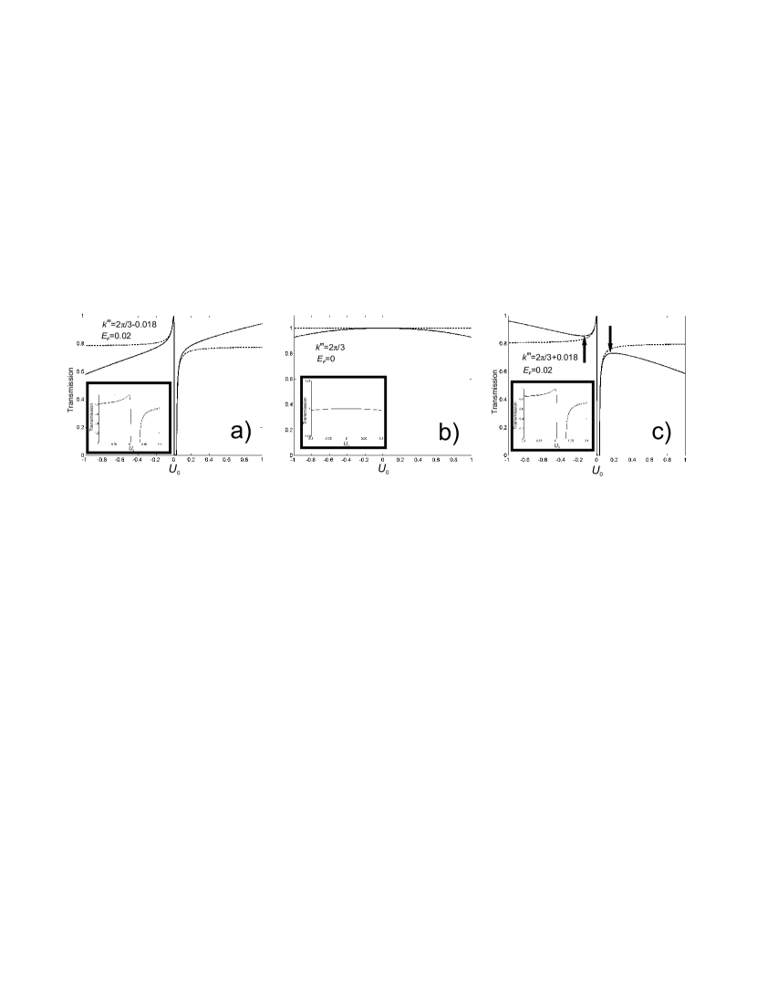
Figure 9: Through-step transmission coefficients versus the applied potential energy $U_{0}$ for three different transverse wave numbers $k^{m}$: a) $k^{m}=2\pi/3-0.018$ and $E_{F}=0.02$; b) $k^{m}=2\pi/3$, $E_{F}=0$; c) $k^{m}=2\pi/3+0.018$, $E_{F}=0.02$. Solid lines correspond to the exact solution (21), dashed lines to the approximate dependence (42). The inserts show the same curves in the low-voltage region $|U_{0}|<0.1$. Two arrows point to the peak and dip of the exact transmission coefficient (21).

When $|U_{0}|<1$, the exact tight-binding solution (21) for $k^{m}=2\pi/3+0.018$, unlike the approximate solution (42), reveals two extreme points, as indicated in the Figure 9c. The existence of such transmission peculiarities follows from the definition (22) an the following chain of identities

$$\frac{dT}{dU_{0}}=\frac{dT}{d\bar{\theta}}\,\frac{d\bar{\theta}}{dU_{0}}=\frac{dT}{d\cos\bar{\theta}}\,\frac{d\cos\bar{\theta}}{dU_{0}}=\frac{dT}{d\cos\bar{\theta}}\,\frac{dg(E-U_{0})}{dU_{0}}=-\frac{dT}{d\cos\bar{\theta}}\,\left.\frac{dg(E)}{dE}\right|_{E\rightarrow E-U_{0}}.$$

Thus, the additional peak and dip of the transmission coefficient are the extreme points of $g(E,k^{m}>2\pi/3)$, $\pm\sqrt{1-4\cos^{2}(k^{m}/2)}$, as discussed in Sec. IX.

It is also important that the exact dependence (21) for $k^{m}\neq 2\pi/3$ predicts unit transmission at applied electrostatic energy $U^{res}_{0}=E_{F}-x/E_{F}$, which is the solution to (32) with respect to $U_{0}$. However, in the case under consideration these resonances are out of the indicated region: $U^{res}_{0}>1$ for $k^{m}<2\pi/3$, and $U^{res}_{0}<-1$ if $k^{m}>2\pi/3$.

Figure 10 depicts the through-barrier transmission coefficients (28) and (43) for the same values of $k^{m}$ and $E_{F}$, as Fig. 9.

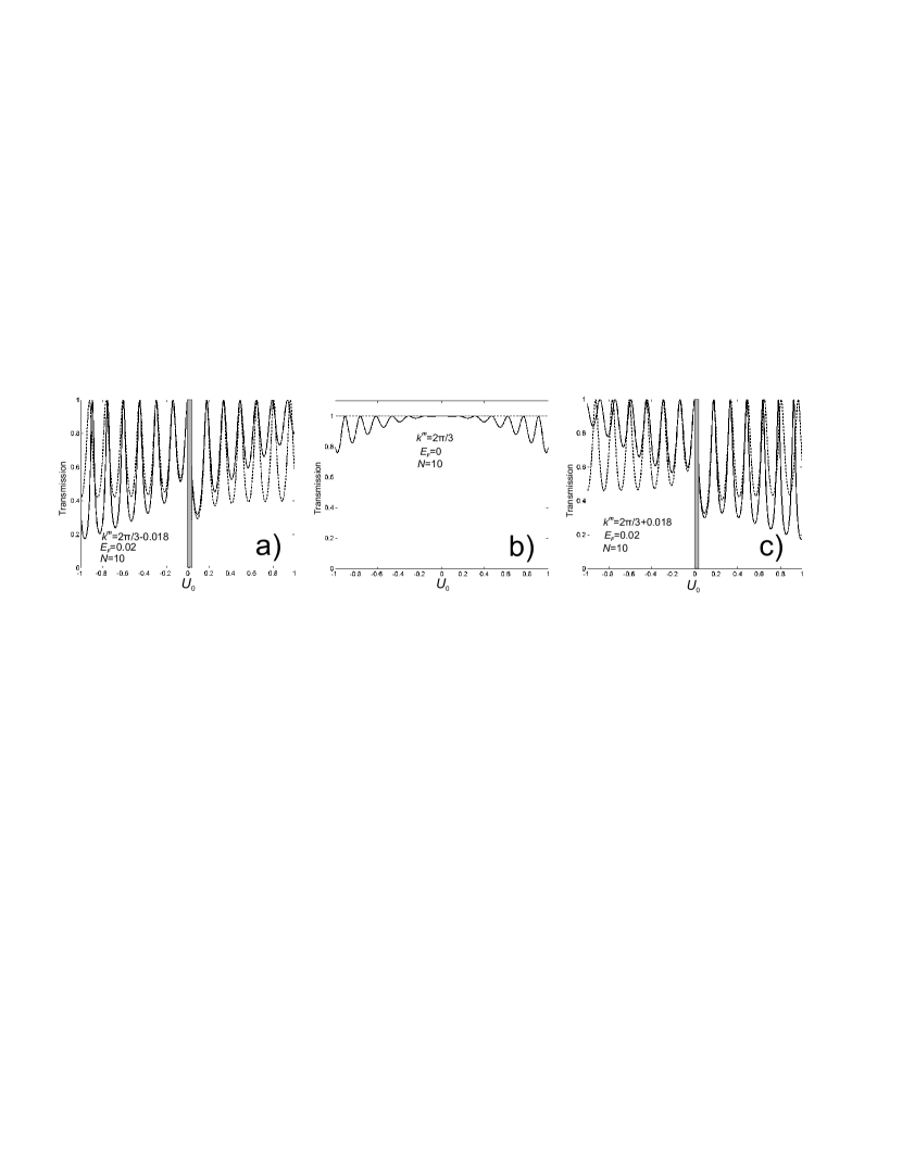
Figure 10: Through-barrier transmission coefficients (28) (solid line) and (43) (dashed line) versus $U_{0}$ calculated for a) $k^{m}=2\pi/3-0.018$ and $E_{F}=0.02$; b) $k^{m}=2\pi/3$, $E_{F}=0$; c) $k^{m}=2\pi/3+0.018$, $E_{F}=0.02$. The grey rectangle is the region of tunneling through a gap which is not studied here.

To make the curves more distinguishable, we consider a narrow barrier, $N=10$. One can see the series of pronounced peaks associated with the resonance conditions $\bar{k}^{n}N\equiv\bar{k}_{x}D=\pi l$ ($l=0,1,\ldots$). A visual comparison of the approximation (43) with the exact solution (28) shows that they are closed to each other in the low-voltage region. However, there are some discrepancies in the resonance positions, especially in the depth of dips outside the low-voltage region. Discrepancies of this kind are also observed between the exact and approximate through-step solutions (21) and (42) over the entire $U_{0}$-region. Formally, if the barrier-induced system is considered as a combination of two scatterers – interfaces between the external and disturbed leads, the through-barrier probability $T^{\rm bar}$ can be written down in terms of the through-step transmission $T^{\rm step}$. The probability $T^{\rm bar}$ varies within the interval defined by (32) from Ref. Klimenko and Onipko (2006)

$$\left(\frac{T^{\rm step}}{2-T^{\rm step}}\right)^{2}\leq T^{\rm bar}\leq 1,$$

which can also be observed from the behaviour of the corresponding through-step coefficient depicted in Fig. 9.

Obviously, as $|k^{m}-2\pi/3|$ increases the exact (tight-binding) and approximate solutions for through-step and through-barrier transmissions in the low-voltage region ($|U_{0}|\ll 1$) are closer to each other. This also follows from Sec. X, specifically from the expansion (44).

Now we consider propagation through a gapless band ($k^{m}=2\pi/3$). Despite visual coincidence of the exact tight-binding solutions with unity in the low-voltage region (Figs. 9b and 10b) the dependences (21) and (28) do not reveal unit propagation for the whole low-voltage region. Thus, the Klein paradox, which strongly predicts that $T=1$ for one-mode propagation through any high and wide potential barriers in semimetal ribbons, fails since the through-step and through-barrier coefficients $T^{{\rm step}({\rm bar})}$ differ from unity though the corresponding deviations are indistinguishable at experimentally reliable values $|U_{0}|\ll 1$.

XII Conclusions

In the framework of the tight-binding model, we present a full and closed description of electron transport in armchair GRs. Starting with the tight-binding Schrödinger equations for a 2D honeycomb lattice, we identify the boundary conditions, wave function and propagation velocity of an electron in armchair GRs. We obtain analytical expressions for the through-step and through-barrier transmission coefficients and demonstrate that new type transmission resonances exist. Such resonances occur when $\cos\theta=\cos\bar{\theta}$, where $\theta$ and $\bar{\theta}$ are the inter-cell electron phase shifts in the corresponding regions. We show that the number and positions of the resonances are strongly dependent on the electron transverse wave number $k^{m}$. In particular, at $k^{m}=2\pi/3$ (propagation through a gapless band), the resonances are absent, and the through-step transmission coefficient reduces to the relation known for through-step propagation in a linear chain of identical atoms. For the low-energy limit, the deviation of the through-step transmission coefficient from unity is proportional to the square of applied potential energy. A similar deviation is also observed for the through-barrier transmission coefficient.

The discrepancy between our tight-binding result and the Klein paradox in graphene becomes evident as a result of expanding the expressions for $\cos\theta$ and $\cos\bar{\theta}$ in the vicinity of the zero-energy point. We show that in the low-energy limit these expressions come to negligibly small terms, which are ignored in the well-known $\bf{k\cdot p}$ method leading to the relativistic Dirac equation. These negligibly small terms ”destroy” unit propagation and produce a small backscattering proportional to $U_{0}^{2}$.

The presented analytical results are in complete agreement with the results of the numerical computations made in the paper.

Appendix A Computation of electron flux

In this appendix, we compute the flux related to electron wave propagation in armchair graphene ribbons. We start with the set of non-stationary Schrödinger equations

$$\begin{array}[]{ll}\left\{\!\!\begin{array}[]{ll}\dot{\psi}_{n,m,l}=-\frac{i\beta}{\hbar}\left[\psi_{n,m,\lambda}+\psi_{n,m+1,\lambda}+\psi_{n-1,m,r}\right],\\ \dot{\psi}_{n,m,\lambda}=-\frac{i\beta}{\hbar}\left[\psi_{n,m,l}+\psi_{n,m,\rho}+(1-\delta_{m,1})\psi_{n,m-1,l}\right],\\ \dot{\psi}_{n,m,\rho}=-\frac{i\beta}{\hbar}\left[\psi_{n,m,\lambda}+\psi_{n,m,r}+(1-\delta_{m,1})\psi_{n,m-1,r}\right],\\ \dot{\psi}_{n,m,r}=-\frac{i\beta}{\hbar}\left[\psi_{n,m,\rho}+\psi_{n,m+1,\rho}+\psi_{n+1,m,l}\right],\end{array}\right.&1\leq m\leq{\cal N},\\ \left\{\!\!\begin{array}[]{l}\dot{\psi}_{n,{\cal N}+1,\lambda}=-\frac{i\beta}{\hbar}\left(\psi_{n,{\cal N}+1,\rho}+\psi_{n,{\cal N},l}\right),\\ \dot{\psi}_{n,{\cal N}+1,\rho}=-\frac{i\beta}{\hbar}\left(\psi_{n,{\cal N}+1,\lambda}+\psi_{n,{\cal N},r}\right).\end{array}\right.&\end{array}$$

Multiplying the equations for $\dot{\psi}_{n,m,\alpha}$ by $\psi^{*}_{n,m,\alpha}$ ($m=1,\ldots,{\cal N}+1$) and adding the obtained relations to the complex conjugated counterparts, and then summing them up over all carbon atoms in unit cell $n$, we get the following

$$\frac{d}{dt}\left[\sum_{m=1}^{{\cal N}}\left\{\left|\psi_{n,m,l}\right|^{2}+\left|\psi_{n,m,r}\right|^{2}\right\}+\sum_{m=1}^{{\cal N}+1}\left\{\left|\psi_{n,m,\lambda}\right|^{2}+\left|\psi_{n,m,\rho}\right|^{2}\right\}\right]=J^{left}+J^{right},$$

where

$$J^{left}=-\frac{i\beta}{\hbar}\sum_{m=1}^{{\cal N}}\left[\psi_{n-1,m,r}\psi^{*}_{n,m,l}-\psi^{*}_{n-1,m,r}\psi_{n,m,l}\right],$$

and

$$J^{right}=-\frac{i\beta}{\hbar}\sum_{m=1}^{{\cal N}}\left[\psi_{n+1,m,l}\psi^{*}_{n,m,r}-\psi^{*}_{n+1,m,l}\psi_{n,m,r}\right].$$

The left side of Eq.(A1) is the rate of change of the electron probability in unit cell $n$. The right side of the equation gives the flux entering to the unit cell. Thus, the flux $J$ outgoing from unit cell $n$ to the right direction equals

$$J=-J^{right}=\frac{i\beta}{\hbar}\sum_{m=1}^{{\cal N}}\left[\psi_{n+1,m,l}\psi^{*}_{n,m,r}-\psi^{*}_{n+1,m,l}\psi_{n,m,r}\right].$$

This formula is used in the main text.

Appendix B Through-step transmission in a linear chain of atoms

In this section, we calculate the through-step transmission coefficient for electron moving in a linear chain of identical atoms (see Fig. 11). For the sake of convenience, we keep the same notation for $E\equiv E/|\beta|$ and $U_{0}=eV_{0}/|\beta|$.

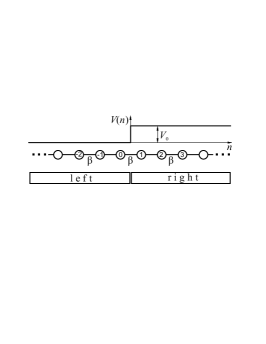
Figure 11: Model of the linear chain of atoms coupled by the electron-transfer integral $\beta$. As in the main text, atoms with $n\leq 0$ correspond to the left lead, and $n\geq 1$ – to the right lead.

Following Fig. 11, we need to determine the solution to the following system of linear Schrödinger equations

$$\left\{\!\!\begin{array}[]{l}-E\psi^{{}^{\rm left}}_{n}=\psi^{{}^{\rm left}}_{n-1}+\psi^{{}^{\rm left}}_{n+1},\quad n<0,\\ -E\psi^{{}^{\rm left}}_{0}=\psi^{{}^{\rm left}}_{-1}+\psi^{{}^{\rm right}}_{1},\\ (U_{0}-E)\psi^{{}^{\rm right}}_{1}=\psi^{{}^{\rm left}}_{0}+\psi^{{}^{\rm right}}_{2},\\ (U_{0}-E)\psi^{{}^{\rm right}}_{n}=\psi^{{}^{\rm right}}_{n-1}+\psi^{{}^{\rm right}}_{n+1},\quad n>1,\end{array}\right.$$

where

$$\psi^{{}^{\rm left}}_{n}=e^{ikn}+re^{-ikn},\qquad\psi^{{}^{\rm right}}_{n}=te^{i\bar{k}n},$$

$r$ and $t$ are the amplitudes of the reflected and transmitted waves, respectively, $k$ and $\bar{k}$ are the non-dimensional wave numbers in the left and right regions. One can see that the first and forth equations in (B1) are satisfied identically if

$$\cos k=-\frac{E}{2},\qquad\cos\bar{k}=-\frac{E-U_{0}}{2}.$$

Plugging in (B2) into the second and third equations from (B1) gives the system of two linear equations

$$1+r=t,\qquad e^{ik}+e^{-ik}\,r=e^{i\bar{k}}\,t.$$

The solution to the system is

$$r=-\frac{e^{i\bar{k}}-e^{ik}}{e^{i\bar{k}}-e^{-ik}},\qquad t=\frac{2i\sin k}{e^{i\bar{k}}-e^{-ik}}.$$

Thus, the transmission coefficient determined as $T=|t|^{2}\sin\bar{k}/\sin k$ can be represented as

$$T=\frac{4\sin k\,\sin\bar{k}}{4\sin k\,\sin\bar{k}+\left(\sin\bar{k}-\sin k\right)^{2}+\left(\cos\bar{k}-\cos k\right)^{2}}.$$

Since the values of $\sin k$ and $\sin\bar{k}$ are positive in the corresponding bands ($0\leq(k,\bar{k})\leq\pi$) one can come to an expression similar to (35) for the transmission coefficient.

Therefore, independently on the Fermi position inside the band, electron propagation through a potential step in a graphene ribbon is described by the same through-step relation as in an undimerized 1D chain with the same ratio $U_{0}=eV_{0}/|\beta|$.

Appendix C Relativistic Dirac solution for the electron reflection probability through a potential barrier.

The reflection amplitude from a potential barrier obtained through the Dirac formalism is described by Eq. (3) in Ref. Katsnelson et al. (2006)

$$r=\frac{2ie^{i\phi}\sin(\bar{k}_{x}D)\,[\sin\phi-ss^{\prime}\sin\bar{\phi}]}{ss^{\prime}\left[e^{-i\bar{k}_{x}D}\cos(\phi+\bar{\phi})+e^{i\bar{k}_{x}D}\cos(\phi-\bar{\phi})\right]-2i\sin(\bar{k}_{x}D)},$$

where $s={\rm sgn}(E)$ and $s^{\prime}={\rm sgn}(E-U_{0})$. Equivalently,

$$r=\frac{ie^{i\phi}\sin(\bar{k}_{x}D)\,[\sin\phi-ss^{\prime}\sin\bar{\phi}]}{ss^{\prime}\cos(\bar{k}_{x}D)\cos\phi\cos\bar{\phi}+i\sin(\bar{k}_{x}D)[ss^{\prime}\sin\phi\sin\bar{\phi}-1]}.$$

Since

$$(1-ss^{\prime}\sin\phi\sin\bar{\phi})^{2}=(\sin\phi-ss^{\prime}\sin\bar{\phi})^{2}+\cos^{2}\phi\cos^{2}\bar{\phi},$$

the reflection probability $R=|r|^{2}$ is given by

$$R=\frac{\sin^{2}(\bar{k}_{x}D)\,[\sin\phi-ss^{\prime}\sin\bar{\phi}]^{2}}{\cos^{2}\phi\cos^{2}\bar{\phi}+\sin^{2}(\bar{k}_{x}D)[\sin\phi-ss^{\prime}\sin\bar{\phi}]^{2}}.$$

Thus, the transmission probability $T=1-R$ through the potential barrier is exactly the same as our approximate relation (43).

References

• Geim and Novoselov (2007) A. K. Geim and K. S. Novoselov, Nature materials 6, 183 (2007).
• Novoselov et al. (2004) K. S. Novoselov, A. K. Geim, S. V. Morozov, D. Jiang, Y. Zhang, S. Dubonos, I. V. Grigorieva, and A. A. Firsov, Science 306, 666 (2004).
• Brey and Fertig (2006) L. Brey and H. A. Fertig, Phys. Rev. B 73, 235411 (2006).
• Fujita et al. (1996) M. Fujita, K. Wakabayashi, K. Nakada, and K. Kusakabe, J. Phys. Soc. Japan 65, 1920 (1996).
• Nakada et al. (1996) K. Nakada, M. Fujita, G. Dresselhaus, and M. S. Dresselhaus, Phys. Rev. B 54, 17954 (1996).
• Wakabayashi et al. (1999) K. Wakabayashi, M. Fujita, H. Ajiki, and M. Sigrist, Phys. Rev. B 59, 8271 (1999).
• Malysheva and Onipko (2008) L. Malysheva and A. Onipko, Phys. Rev. Lett. 100, 186806 (2008).
• Ezawa (2006) M. Ezawa, Phys. Rev. B 73, 045432 (2006).
• Robinson and Schomerus (2007) J. P. Robinson and H. Schomerus, Phys. Rev. B 76, 115430 (2007).
• Schomerus (2007) H. Schomerus, Phys. Rev. B 76, 045433 (2007).
• Peres et al. (2006) N. M. R. Peres, A. H.  Castro Neto, and F. Guinea, Phys. Rev. B 73, 195411 (2006).
• Ando et al. (1998) T. Ando, T. Nakanishi, and R. Saito, J. Phys. Soc. Japan 67, 2857 (1998).
• Ando (2002) T. Ando, J. Phys. Soc. Japan 74, 777 (2002).
• Tworzydlo et al. (2006) J. Tworzydlo, B. Trauzettel, M. Titov, A. Rycerz, and C. W. J. Beenakker, Phys. Rev. Lett. 96, 246802 (2006).
• Katsnelson et al. (2006) M. I. Katsnelson, K. S. Novoselov, and A. K. Geim, Nature Physics 2, 620 (2006).
• Wakabayashi et al. (2007) K. Wakabayashi, Y. Takane, and M. Sigrist, Phys. Rev. Lett. 99, 036601 (2007).
• Katsnelson (2006) M. I. Katsnelson, Eur. Phys. J. B 51, 157 (2006).
• Pereira et al. (2007) J. M. Pereira, P. Vasilopoulos, and F. M. Peeters, Appl. Phys. Lett. 90, 132122 (2007).
• Silvestrov and Efetov (2007) P. G. Silvestrov and K. B. Efetov, Phys. Rev. Lett. 98, 016802 (2007).
• Barbier et al. (2008) M. Barbier, F. M. Peeters, P. Vasilopoulos, and J. M. Pereira, Phys. Rev. B 77, 115446 (2008).
• Cheianov and Fal’ko (2006) V. V. Cheianov and V. I. Fal’ko, Phys. Rev. B 74, 041403(R) (2006).
• Zheng et al. (2007) H. Zheng, Z. F. Wang, T. Luo, Q. W. Shi, and J. Chen, Phys. Rev. B 75, 165414 (2007).
• Akhmerov and Beenakker (2008) A. R. Akhmerov and C. W. J. Beenakker, Phys. Rev. B 77, 085423 (2008).
• Onipko et al. (1997) A. Onipko, Y. Klymenko, , and L. Malysheva, J. Chem. Phys 107, 5032 (1997).
• Klimenko and Onipko (2006) Y. A. Klimenko and A. I. Onipko, Low Temp. Phys. 20(9), 721 (2006).