Geometry reconstruction of fluorescence detectors revisited
Abstract
The experimental technique of fluorescence light observation is used in current and planned air shower experiments that aim at understanding the origin of ultra-high energy cosmic rays. In the fluorescence technique, the geometry of the shower is reconstructed from the correlation between arrival time and incident angle of the signals detected by the telescope. The calculation of the expected light arrival time used so far in shower reconstruction codes is based on several assumptions. Particularly, it is assumed that fluorescence photons are produced instantaneously during the passage of the shower front and that the fluorescence photons propagate on a straight line with vacuum speed of light towards the telescope. We investigate the validity of these assumptions, how to correct them, and the impact on reconstruction parameters when adopting realistic conditions. Depending on the relative orientation of the shower to the telescope, corrections can reach 100 ns in expected light arrival time, 0.1∘ in arrival direction and 5 g cm-2 in depth of shower maximum. The findings are relevant also for the case of “hybrid” observations where the shower is registered simultaneously by fluorescence and surface detectors.
v2.0
1 Introduction
Understanding the origin and nature of ultra-high energy (UHE) cosmic rays above eV is a major challenge of astroparticle physics [1]. These cosmic rays are studied by detecting the atmospheric showers they initiate. Current and planned air shower experiments [2, 3, 4, 5, 6] use the technique of fluorescence light observation: shower particles deposit energy in the atmosphere through ionisational energy loss. Part of this energy (of order ) is emitted isotropically at near-UV wavelengths in de-excitation processes. These fluorescence photons can be detected by appropriate telescope systems operating in clear nights. Typically, pixel cameras with 25100 ns timing resolution are used, where an individual pixel covers a field of view of about 11.5∘ in diameter (see e.g. Ref. [2]). The signal (light flux per time) is registered as a function of the viewing direction of the pixels.
The first step to reconstruct the primary parameters of an observed air shower is given by the determination of the shower geometry. An accurate geometry reconstruction is, for instance, decisive for directional source searches; but it is also a prerequisite for reconstructing other important shower parameters such as the primary energy or the depth of shower maximum. We note that also the shower energies obtained from Auger ground array data are calibrated by the fluorescence telescopes [7].
The determination of the shower geometry is commonly performed in two steps in the fluorescence technique [9]. First, the “shower-detector-plane” (SDP) is determined as the plane spanned by the (signal-weighted) viewing directions of the triggered camera pixels (Fig. 1). Next, the geometry of the shower within this SDP is reconstructed based on the correlation between arrival time of the signals and viewing angle of the pixels projected into the SDP. The measured time-angle correlation is compared to the one expected for different shower geometries, and the best-fit geometry is determined. For the calculation of the expected time-angle correlation, the following function is in use (following e.g. Ref. [8, 9, 10]):
| (1) |
where is the arrival time of the photons at camera pixel (usually, a signal-weighted average arrival time is taken from the time sequence observed in a pixel), is the time at which the shower axis vector passes the closest point to the telescope at a distance , is the vacuum speed of light, is the angle of incidence of the shower axis within the SDP, and is the viewing angle of pixel within the SDP (see also Fig. 1). Comparing the expected correlation to the observed one ( for triggered pixels), the best-fit parameters , and in Eq. (1) are found by a -minimization. Together with the SDP derived previously, the shower geometry is then fully determined and can also be expressed in terms of shower impact point, arrival direction, and ground impact time.
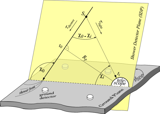
Eq. (1) is derived as follows. Assuming the fluorescence light to be emitted by a point-like object moving at along the shower axis vector, the shower propagation time from point to the point at reference time on the shower axis (Fig. 1) can be expressed as
| (2) |
Next, assuming the fluorescence photons to propagate on straight lines with , the light propagation time from to the telescope is
| (3) |
With Eqs. (2) and (3), and assuming an instantaneous emission of the fluorescence photons at , the expected arrival time (relative to the time of closest approach of the shower to the telescope) of fluorescence photons at a pixel viewing at an angle becomes
| (4) | |||||
which equals Eq. (1).
Thus, the derivation of Eq. (1) for calculating the expected time-angle correlation is based on the following assumptions:
-
•
the spatial structure and the propagation of the shower disk can be approximated by a point-like object moving at ,
-
•
the fluorescence light is produced instantaneously,
-
•
the fluorescence light propagates with ,
-
•
the fluorescence light propagates on a straight line.
In this article, we investigate the validity of these assumptions. The impact of the corrections on reconstruction parameters is studied. The results are relevant both for observations with fluorescence telescopes alone and for “hybrid” observations where the shower is registered by fluorescence and surface detectors.
2 Analysis of individual effects
We discuss step-by-step the individual effects given by
-
•
the spatial structure and speed of the shower disk (instead of a point-like object moving with ),
-
•
the delayed (instead of instantaneous) fluorescence light emission,
-
•
the reduced propagation speed of light (instead of ),
-
•
the bending of light (instead of straight-line propagation).
2.1 Spatial structure and speed of shower disk
To check the assumption of the shower propagating as a point-like object with on a straight line, one may first regard the fastest particles during the cascading process. Assuming, as a rough estimate, an elasticity of 50% per interaction, the energy of the leading particle in a hadronic air shower is after interactions for a primary particle of energy and mass . For (the depth of shower maximum in units of the hadronic interaction length), the energy of the leading particle is for primary protons and of order for primary iron. Hence, eV for primary energies eV around shower maximum, which is the most relevant portion of the shower development for fluorescence light observations. In this case, the accumulated time delay of the leading particles with respect to an imaginary shower front moving with from the first interaction to is 1 ns. This is negligible compared to current timing resolutions of giant shower detectors. Lateral deflections of these particles due to transverse momenta in interactions or deflection in the Earth’s magnetic field are also sufficiently small (below 1 m).111 Time delay and lateral deflection of the leading particles may become non-negligible in case of considerably smaller or larger (the latter being rather relevant for ground array observations of near-horizontal showers). For the case of UHE shower observations by fluorescence telescopes we conclude that the fastest shower particles can in reasonable approximation be assumed to move on a straight line along the shower axis with .
The main contribution to the fluorescence signal in the shower, however, is due to lower-energy secondaries, particularly electrons and positrons between 0.1 MeV and several 100 MeV [11].222Note that for the energy transfer from MeV electrons to fluorescence photons, the production of even lower-energy (e.g. keV) electrons is important (for instance, the cross-section for exciting the main molecular bands (cf. Section 2.2) has a sharp peak at about 20 eV electron energy). However, the additional delay from this intermediate step is ns and, thus, negligible for this analysis [12]. These have larger lateral displacements from the shower axis and larger longitudinal time delays with respect to the shower front.
Concerning the lateral width of the fluorescence shower beam, about 80% of the total fluorescence signal is produced within 75 m around the shower axis [11]. The impact of the finite shower width on the fluorescence reconstruction and how to correct it, was previously studied in detail [13]. It was shown in Ref. [13] that choosing too small a photon collection angle around the shower axis during reconstruction can lead to a signal loss and underestimation of the primary energy in nearby showers.
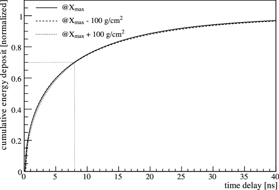
Here we study the longitudinal time delay of secondaries using the CORSIKA code [14]. In Fig. 2 the time delay of secondaries, weighted according to their contribution to the energy release into air and thus to the fluorescence signal, after the arrival time of the first particles is shown (1019 eV shower at maximum, for particles closer than 75 m from the axis; results are practically identical for primary proton and iron showers). One can note a sharp initial increase of the cumulative distribution (about 50% of energy is deposited within the first 34 ns after the fastest particle), with a long tail towards larger delays. The average time delay is 8 ns, corresponding to a shower “thickness” of a few meters, which is in reasonable agreement with measurements of particle delays in air showers (see e.g. Ref. [15]). As can also be seen in Fig. 2, the distribution of time delays changes only marginally with the shower development stage.
The delay of secondaries with respect to the fastest shower particles results in a small constant time offset of the observed shower compared to the assumption of the shower moving with . This might be less relevant for observations with fluorescence telescopes alone, since in this case, only the relative timing between the pixels is used to determine the spatial shower geometry. For hybrid observations, however, usually the arrival time of the first particle in the ground detector is taken, while in fluorescence telescopes, usually an average time from a fit to the signal viewed by a pixel is used. Then, comparing the timing signals from ground and fluorescence detectors, the small shift due to the finite shower thickness should be taken into account.333For ground detectors located at larger distances from the shower axis, the curvature of the shower front needs to be accounted for in addition. The precise value of the delay will depend on the specific procedure of signal extraction applied during reconstruction. As a rough estimate, the delay is of order 6 ns.
To summarize, the leading particles in 1018 eV showers can be considered to propagate along the shower axis with , and one can set with given by Eq. (2). Compared to these particles, the secondaries relevant for the fluorescence light are slightly delayed due to the finite shower thickness by , i.e. this term has to be added on the r.h.s. of Eq. (4).
2.2 Fluorescence light production
During propagation, the shower particles excite and ionize air molecules. Fluorescence light is then emitted by de-excitation and recombination. Most of the fluorescence light originates from transitions from the second positive system (2P) of molecular nitrogen N2 and the first negative system (1N) of ionized nitrogen molecules [8].
Typical excitation times are of the order ns [17] and negligible for current fluorescence telescopes. De-excitation times, in turn, can exceed 30 ns. Depending on the local atmospheric conditions and on the specific transition system, quenching processes (radiationless transitions by collisions with other molecules) can substantially reduce the mean de-excitation time of the radiative processes.
The total reciprocal lifetime of an electronic vibrational state can be expressed as a function of pressure and temperature as (see e.g. Ref. [18] and references therein)
| (5) |
Here, is the reciprocal intrinsic lifetime defined as the sum of all constant transition probabilities and is a reference pressure for a given gas mixture defined as the pressure where the collisional deactivation constant equals the reciprocal intrinsic lifetime [18].
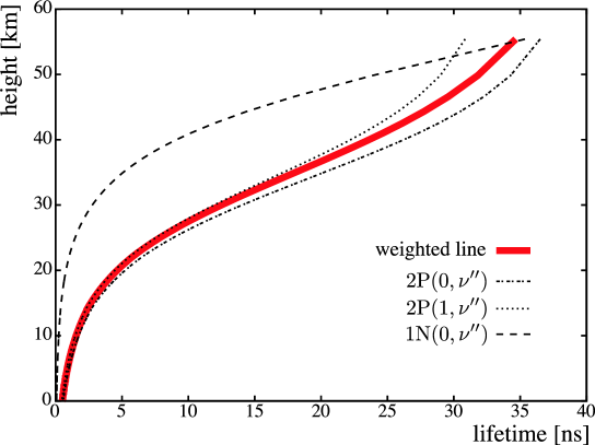
Fig. 3 shows the calculated lifetimes as a function of height for the three main sets of bands 2P, 2P and 1N, assuming dry air ( N2, O2 and Ar) and temperature profiles corresponding to the typical conditions at the Auger Observatory [19]. Also shown is the averaged lifetime, weighting the emission bands according to their relative (altitude dependent) intensities. The width of the weighted line indicates the effect of an arbitrary temperature variation of 40 K to show the minor dependence of the averaged lifetime on reasonable variations of the actual atmospheric conditions. At very high altitudes of 3040 km, the averaged lifetime is 1525 ns. With decreasing altitude, the quenching effect reduces the lifetime; thus, in general, the delay of fluorescence light emission with respect to the passing shower front is a differential effect that changes during the shower development (smaller delay deeper in the atmosphere).444Anecdotally, this means the front of fluorescence light emission can move with an apparent velocity larger than through the atmosphere. At heights below 20 km where showers are typically observed by ground-based observatories, lifetimes of a few ns are reached.
2.3 Reduced speed of light
The propagation speed of light is reduced compared to the vacuum case by the local index of refraction of air . The change of with wavelength is small (3%) [20] within the fluorescence window of about 300400 nm. Following Ref. [21], the index of refraction can be parametrized as a function of altitude as
| (7) |
with the atmospheric density profile ; and are the reference values at sea level. The propagation time of refracted light over a small line element is then given by and for propagation between two points at altitudes and () by
| (8) |
with being the zenith angle of the propagation direction of light.
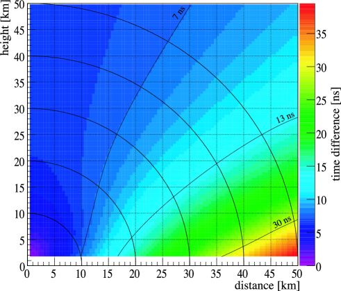
In Fig. 4, the difference of light arrival times (between the cases of vacuum and reduced speed of light) is shown as a function of the location of emission point with respect to a telescope. The parametrization of is taken from Ref. [19] for the example of the southern Auger Observatory. As expected, for fixed distance between emission point and telescope, time differences grow for propagation closer to ground due to the larger value of . Differences of 2025 ns or more can occur. For a single air shower, the effect changes along the longitudinal shower path, depending also on the relative orientation of shower axis and telescope. For instance, the time difference along the shower path typically varies less for showers pointing towards the telescope.
In Eq. (4), is replaced by . For convenience, one can express using Eq. (3) by replacing with , defined as the effective speed of refracted light along the path of length between emission point and telescope.
2.4 Bending of light
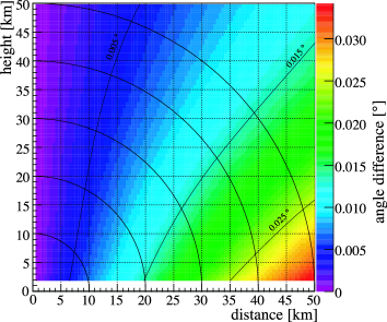
Due to refraction, the emitted light propagates on a bent trajectory. In turn, the direction of the incidence angle of the observed light does not point towards the real emission point, see Fig. 5 (right). More specifically, the zenith angle of down-going light is continuously reduced during propagation.555We consider here only the case of a stable atmosphere with a standard decrease of and with height as given by Eq. (7) and Ref. [19]. We note, however, that the path of refracted light can become more complicated for specific atmospheric conditions such as atmospheric inversion, or in case of a strongly radiating ground leading to a local heating of air. The impact of the latter on the fluorescence technique might be reduced due to the fact that observations are only performed well (12 h) after / before sunset; also, the shower path very close to ground usually is below the field of view of the telescope (1∘ elevation of lower edge of field of view). The zenith angle difference between the observed light direction (towards the apparent emission point) and the straight-line direction (towards the real emission point) has been calculated from ray tracing with from Eq. (7); it is shown in Fig. 5 (left) as a function of the position of the emission point in the atmosphere relative to the telescope. As an example, an angular difference of 0.02∘ implies a 12 m upward shift of the apparent emission point for a vertical shower at 30 km distance which corresponds to a 40 ns shift in time. These shifts change over the longitudinal viewing direction towards an air shower. In case of hybrid observations where timing signals of fluorescence and ground detectors are combined, the impact time on ground estimated from the telescopes will be delayed compared to the actual one.
For a vertical shower, or, more generally, for showers with (cf. Fig. 1), in Eq. (4) is just reduced by , as the refracted light direction still points towards the actual shower axis. In general, however, this effect slightly shifts the refracted light signals out of the actual SDP, and this shift usually changes along the shower path. Thus, the apparent SDP (which, in fact need not be a “plane” anymore) may slightly be tilted compared to the real one. To still permit the practical approach of fitting the best shower geometry within a plane only (instead of testing the full phase space), the projected shift is taken as a correction. Thus, in Eq. (4), is replaced by where denotes the effective viewing direction of pixel due to refraction. To account for the possible slight tilt of the apparent SDP, which is expected to be no larger than (few times) 0.01∘, the best-fit SDP might be found in an iterative procedure.
Finally, we note that the additional time delay due to the increased, bent path length compared to the straight-line connection (see sketch in Fig. 5) is 1 ns and can thus be neglected.

3 Impact on shower reconstruction
Taking the discussed effects into account, Eq. (1) is finally replaced by
| (9) |
The index indicates that these quantities, for a given shower geometry, depend on the viewing direction of pixel . One caveat, as discussed in Sec. 2.4, is that the bending of light slightly changes the apparent SDP (within which the angles and are defined). It is worthwhile to note that all correction terms depend only on shower geometry but not on shower physics such as the primary particle type, which facilitates their application in shower reconstruction codes. can, to a good degree, be treated as a constant; depends on the altitude of the emission point; and and depend on the locations of emission point and telescope.
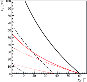
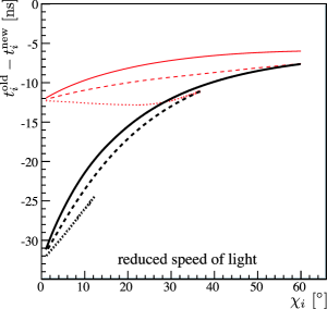
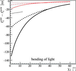
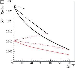
The time shifts introduced by the various effects along the viewing direction towards the shower are displayed in Fig. 6 for different shower geometries. The distance between impact point and telescope were fixed to 15 km (thin line) and 40 km (thick line), and for each distance three different shower inclinations of are considered. Here, for simplicity is taken such that is identical to the shower zenith angle. In this case, the effect from light bending is minimized concerning the change of the SDP and maximized concerning .
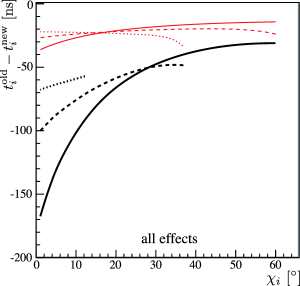
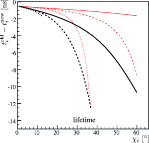
In Fig. 6 (a), the overall shapes of vs. are given, which differ for the different geometries. The shift of the arrival times, compared to the previous approach, is shown in Fig. 6 (b) when taking all effects into account. The contributions from the individual effects are provided in Figs. 6 (c)(e). For the bending of light, in Fig. 6 (f), also the shift between apparent and effective viewing angle is given. One sees that the time delays are geometry dependent and can reach, and even exceed, 50100 ns.
One also sees in Fig. 6 that the time delays change along the shower track in an individual event. When reconstructing the shower as a whole, the fitting procedure then minimizes the overall by adjusting simultaneously , and . To investigate the effective impact of the corrections on the final reconstruction parameters, events were generated using CORSIKA [14] with the hadronic interaction model QGSJET 01 [16]. The shower sample consists of proton induced showers with energies of , and eV and zenith angles of 0, 45 and 60 deg (100 events per combination with random azimuth angles). The detector simulation and the event reconstruction was performed using the Auger software package described in [22, 23]. These data were reconstructed with and without accounting for the discussed effects; or, more specifically, using once Eq. (1) and once Eq. (9) in the reconstruction, and comparing the differences.
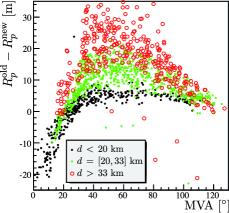
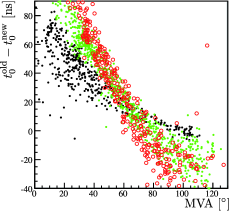
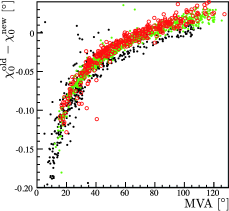
As the time delays from individual parts of the shower were found to depend on distance and relative orientation of the shower to the telescope, we plot in Fig. 7 the change in the parameters , and as a function of the minimum viewing angle (MVA), divided in different distance bins. The MVA is defined as the smallest angle under which the reconstructed air shower is seen by the telescope. Some dependence on MVA and distance can indeed be seen, as expected also from projection effects (for instance, a given angular offset in viewing direction leads to a larger shift along the shower axis for showers pointing towards the telescope than for vertical showers), or from an accumulation of certain effects with distance (such as the time delay due to the reduced speed of light). The actual impact of the corrections on an individual event is more complex, however, and has some dependence also on parameters other than geometry. For instance, the shower track of a higher-energy event can be observed out to larger altitudes due to the increased light output, such that these parts of the shower track can also contribute to the geometry fit. Thus, an a posteriori correction of the geometry parameters determined with Eq. (1) is not straightforward and would neglect individual event properties.
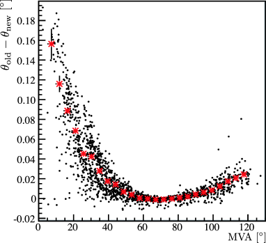
For values of the MVA larger than 4050∘, deviations up to about 15 m (in ), 30 ns (in ), and 0.04∘ (in ) are observed. Differences in are typically larger in case of more distant showers. At smaller values of the MVA (showers pointing towards the telescope), also larger deviations are possible, e.g. shifts in of 0.1∘ or more. In terms of differences in arrival directions (the relevant quantity for directional source searches), differences are typically around 0.05∘, but can exceed 0.1∘. A systematic shift can be noted to slightly overestimate the shower zenith angles when neglecting the discussed effects, see Fig. 8. Shifts in energy are usually small ( 0.51% on average). Reconstructed values for the depth of shower maximum are typically changed by 23 g cm-2, with a trend of the corrected values being increased, and with larger corrections (5 g cm-2 and more) towards smaller values of MVA.
4 Conclusion
The assumptions used in the “classical” function of Eq. (1) for reconstructing the shower geometry from fluorescence light observations were investigated. The finite shower thickness leads to an energy deposition in air by secondaries which is delayed, compared to the shower front, by about 56 ns (with some dependence on the specific light collection algorithm employed). The emission of fluorescence light is further delayed due to the finite lifetime of the transitions which, due to quenching, is altitude dependent. Typical values are a few nanoseconds up to 20 km height, and 15 ns for heights above 30 km. The propagation speed of light is reduced by the index of refraction of air. The delay, compared to a propagation with vacuum speed of light, depends on the locations of emission point and telescope, and can exceed 2025 ns. Finally, another effect of refraction is the bending of light, which also depends on the locations of emission point and telescope. Angular differences between the apparent and actual emission point of 0.02∘ can occur, which may correspond to time shifts of several 10 ns. This effect can also lead to a slight tilt of the SDP.
All these corrections can be considered as geometrical ones, i.e. they are independent of specific properties of the individual showers other than their geometry. The corrected function for geometry reconstruction is given in Eq. (9). Compared to the previous approach, which assumed maximum propagation speed of both light and particles as well as no other delays, the effects of delayed timing (including the effect of bending of light) accumulate. In total, differences of up to 100 ns in estimated light arrival time are possible. Air shower experiments with comparable, or better, time resolution should take these effects into account. This refers both to data reconstruction and to implementing these effects in the showerdetector simulation. In terms of overall shower reconstruction parameters, corrections are typically 0.030.05∘ in arrival direction (with a systematic trend of overestimating the zenith angle when neglecting the effect), 0.51% in energy and 23 g cm-2 in , but may in some cases exceed 0.1∘ and 5 g cm-2. This is to be compared to typical reconstruction accuracies of 0.6∘ (directional resolution) [24] and 11 g cm-2 (systematic uncertainty) [25] in case of Auger hybrid events.
The increase in computing time for event reconstruction is modest, particularly when applying the corresponding corrections only when approaching convergence in the minimization process (increase of 20% or less, depending on implementation). Some of the effects investigated in this work might be relevant also for shower detection techniques other than fluorescence telescope observations at ultra-high energy, e.g. Cherenkov light observations of air showers.
Acknowledgements:
We would like to thank our Colleagues from the Pierre Auger Collaboration for many fruitful discussions, in particular Fernando Arqueros, Jose Bellido, Bruce Dawson, Philip Wahrlich and the members of the Auger group at the University of Wuppertal. Figs. 7 and 8 were produced using Auger software packages [22, 23]. This work was partially supported by the German Ministry for Research and Education (Grant 05 CU5PX1/6).
References
- [1] M. Nagano, A.A. Watson, Rev. Mod. Phys. 72, 689 (2000); “Ultimate energy particles in the Universe,” eds. M. Boratav and G. Sigl, C.R. Physique 5, Elsevier, Paris (2004); J. Cronin, Nucl. Phys. B, Proc. Suppl. 138 (2005), 465
- [2] J. Abraham et al., P. Auger Collaboration, Nucl. Instrum. Meth. A 523, 50 (2004)
- [3] R.U. Abbasi et al., Phys. Lett. B 619, 271 (2005)
- [4] M. Fukushima et al., Prog. Theor. Phys. Suppl. 151, 206 (2003)
- [5] http://www.euso-mission.org
- [6] http://owl.gsfc.nasa.gov
- [7] M. Roth for the Pierre Auger Collaboration, Proc. 30th Intern. Cosmic Ray Conf., Merida (2007); arXiv:0706.2096 [astro-ph]
- [8] A. N. Bunner, “Cosmic Ray Detection by Atmospheric Fluorescence,” Ph.D. thesis, Graduate School of Cornell University, (1967)
- [9] R. M. Baltrusaitis et al., Nucl. Instrum. Meth. A 240, 410 (1985)
- [10] P. Sokolsky, “Introduction to Ultrahigh Energy Cosmic Ray Physics,” Addison-Wesley, Redwood City, USA (1989)
- [11] M. Risse and D. Heck, Astropart. Phys. 20, 661 (2004)
- [12] F. Arqueros, private communication (2008)
- [13] D. Góra et al., Astropart. Phys. 24, 484 (2006)
- [14] D. Heck et al., Reports FZKA 6019 & 6097, Forschungszentrum Karlsruhe (1998)
- [15] G. Agnetta et al., Astropart. Phys. 6, 301 (1997)
- [16] N.N. Kalmykov, S.S. Ostapchenko, A.I. Pavlov, Nucl. Phys. B (Proc. Suppl.) 52B, 17 (1997)
- [17] T. Waldenmaier, “Spectral resolved measurement of the nitrogen fluorescence yield in air induced by electrons,” FZKA-7209, Forschungszentrum Karlsruhe, (2006)
- [18] T. Waldenmaier et al., Astropart. Phys. 29, 205 (2008)
- [19] B. Keilhauer et al. [Pierre Auger Collaboration], arXiv:astro-ph/0507275.
- [20] K. Bernlöhr, Astropart. Phys. 12, 255 (2000)
- [21] R. C. Weast (ed.), “Handbook of Chemistry and Physics,” 51st edition (Chemical Rubber Co., 1963) p. E-231
- [22] S. Argiro et al., Nucl. Instr. Meth. A580, 1485 (2007)
- [23] L. Prado et al., Nucl. Instr. Meth. A545, 632 (2005)
- [24] C. Bonifazi for the Pierre Auger Collaboration, Proc. 29th Intern. Cosmic Ray Conf., Pune, 7, 17 (2005)
- [25] M. Unger for the Pierre Auger Collaboration, Proc. 30th Intern. Cosmic Ray Conf., Merida (2007); arXiv:0706.1495 [astro-ph]