Quantum chaos; semiclassical methods Decoherence; open systems; quantum statistical methods Quantum information

Quantum chaotic system as a model of decohering environment

Abstract

As a model of decohering environment, we show that quantum chaotic system behave equivalently as many-body system. An approximate formula for time-evolution of the reduced density matrix of a system interacting with a quantum chaotic environment is derived. This theoretical formulation is substantiated by numerical study of decoherence of two qubits interacting with a quantum chaotic environment modeled by chaotic kicked top. Like many-body model of environment, quantum chaotic system is efficient decoherer, and it can generate entanglement between the two qubits which have no direct interaction.

Interaction of a quantum system with environment creates correlations between the states of the system and of the environment. These correlations destroy the superposition of the system states - a phenomenon known as decoherence [1]. This phenomenon is believed to be responsible for quantum to classical transition. Decoherence is also a major obstacle for designing quantum computational and informational protocol [2]. Therefore, a deeper understanding of the phenomenon is required to address the fundamental question like quantum-classical transition and, to develop quantum computational protocol.

In general, the environment is modeled by many-body system, e.g. infinitely many harmonic oscillators in thermal equilibrium (Feynman-Vernon or Caldeira-Leggett model) [3], spin-boson model [4], chaotic spin-chain [5], etc. In another approach, random matrix model of the environment is used [6, 7]. Random matrix theory has well known connections with quantum chaotic systems. Hence, some studies have concentrated on the possibility of having quantum dissipation and decoherence due to the interaction with chaotic degrees of freedom [8]. Recently, as a model of decohering environment, single particle quantum chaotic system has been considered [9]. This paper shows that the kicked rotator, a well studied model of chaotic system, can reproduce the decohering effects of a many-body environment. In comparison to complex many-body system, this simple deterministic system is very convenient for numerical as well as analytical studies of decoherence. Hence, single particle quantum chaotic system warrants a special attention as a model of decohering environment.

In this Letter, we establish direct equivalence of single particle quantum chaotic environment and Caldeira-Leggett type model of many-body environment by providing a rigorous but straightforward treatment. We keep our results vis-a-vis a recent study in which decoherence in a quantum system is investigated under the influence of a collection of harmonic oscillators environment [10]. Our derivation first assumes weak interaction between the system and the environment. Using the interaction strength as a small parameter, we perform perturbative theory calculation. By exponentiating the perturbative expansion, we get an approximate formula for the non-perturbative strong interaction effect of the environment on the system. The approximate formula is then justified by numerical evidences. In numerics, we study decoherence of two noninteracting qubits which are individually interacting with a common quantum chaotic environment. We use chaotic kicked top, a very well studied model of quantum chaotic system [11], as the environment.

Most general form of the Hamiltonian of a system $S$, interacting with an environment $E$, is $H=H_{S}+H_{E}+H_{SE}$, where $H_{S}$ and $H_{E}$ are the Hamiltonians of the system and the environment, respectively, and $H_{SE}$ is the system-environment coupling Hamiltonian. We assume throughout this Letter that the decoherence time is much smaller than the system characteristic time. Hence we can neglect any dynamics of the isolated system and can discard $H_{S}$. We consider kicked quantum chaotic system as a model of the environment, so the general form of the time-dependent system-environment Hamiltonian is : $H(t)=I_{S}\otimes H_{E}(t)+H_{I}(t)$ where $H_{E}(t)=H_{1}+H_{2}\sum_{n}\delta(t-n)$ and $H_{I}(t)=\alpha V_{S}\otimes V_{E}$; $V_{S}$ and $V_{E}$ are the coupling agents of the system and the environment, respectively. Parameter $\alpha$ determines the strength of the interaction. We now assume that $V_{E}$ commutes with $H_{1}$. This is a very natural assumption as it separates environment dynamics from the system-environment interaction. The corresponding time-evolution operator $U$ in between two consecutive kicks is: $U=U_{I}U_{0}=U_{I}(I_{S}\otimes U_{E})$, where the coupling part $U_{I}=\exp(-i\alpha V_{S}\otimes V_{E})$, $I_{S}$ is a unit matrix which indicates the absence of any dynamics in the system, and $U_{E}=\exp(-iH_{1})\exp(-iH_{2})$. Further, we assume that the initial joint state of the system-environment is an unentangled pure state of the form $|\Psi_{SE}(0)\rangle=|\psi_{S}(0)\rangle\otimes|\psi_{E}(0)\rangle$. We measure decoherence of the system by its loss of purity $P(n)\equiv\mbox{Tr}_{S}[\rho_{S}(n)^{2}]$ which varies from $1$, for pure state, to $1/N_{S}$ for completely mixed state, $N_{S}$ being the Hilbert space dimension of $S$. And $\rho_{S}(n)\equiv\mbox{Tr}_{E}|\Psi_{SE}(n)\rangle\langle\Psi_{SE}(n)|$ is the system reduced density matrix (RDM), where $|\Psi_{SE}(n)\rangle$ is the joint state of the system and the environment at time $n$.

We are interested to study entanglement between the two non-interacting qubits due to their interaction with a common chaotic environment. Following Wootters, the entanglement is measured by computing the concurrence $C[\rho_{S}(n)]=\max(\Lambda,\,0)$, where $\Lambda\equiv\sqrt{\lambda_{1}}-\sqrt{\lambda_{2}}-\sqrt{\lambda_{3}}-\sqrt{\lambda_{4}}$ and $\lambda_{i}$’s are the eigenvalues of the matrix $R(n)=\rho_{S}(n)\widetilde{\rho_{S}(n)}$; $\widetilde{\rho_{S}(n)}\equiv(\sigma_{y}\otimes\sigma_{y})\rho_{S}(n)^{\star}(\sigma_{y}\otimes\sigma_{y})$, $\rho_{S}(n)^{\star}$ being the complex conjugation of $\rho_{S}(n)$ in the computational basis $\{|00\rangle,|01\rangle,|10\rangle,|11\rangle\}$ [12]. The concurrence varies from $0$, for separable state, to $1$ for maximally entangled state.

Our perturbation theory approach is reminiscent of the method followed by Tanaka et. al. in the context of entanglement production between two coupled chaotic systems [13]. We define the interaction picture of the joint density matrix $\overline{\rho_{SE}}(n)\equiv U_{0}(n)^{\dagger}\rho_{SE}(n)U_{0}(n)$, and of any arbitrary operator $O(n)\equiv U_{0}(n)^{\dagger}OU_{0}(n)$, where $U_{0}(n)\equiv(I_{S}\otimes U_{E})^{n}$, and $O(n)$ represents the free evolution of $O$. Thus, the time evolution of $\overline{\rho_{SE}}(n)$ is determined by the mapping : $\overline{\rho_{SE}}(n)=U_{I}(n)\overline{\rho_{SE}}(n-1)U_{I}(n)^{\dagger}$. The perturbative expansion for $U_{I}(n)$ is :

$$U_{I}(n)=1-i\alpha V(n)-\frac{1}{2}\alpha^{2}V(n)^{2}+\mathcal{O}(\alpha^{3}),$$ (1)

where $V(n)\equiv V_{S}(n)\otimes V_{E}(n)$, $V_{S}(n)$ and $V_{E}(n)$ are as usual free evolutions of $V_{S}$ and $V_{E}$, respectively. We introduce the eigenvalues and the eigenvectors of $V_{S}$ as $V_{S}|s\rangle=\lambda_{s}|s\rangle$. By tracing out the environment, we obtain perturbative expansion of RDM of the system $S$ at time $n$ in the eigenbasis of $V_{S}$ upto $\mathcal{O}(\alpha^{2})$ as :

$$\left[\rho_{S}(n)\right]_{ss^{\prime}}\simeq\left[1-i\,\alpha(\lambda_{s}-\lambda_{s^{\prime}})g(n)-\frac{1}{2}\alpha^{2}(\lambda_{s}-\lambda_{s^{\prime}})^{2}g(n)^{2}\right.$$

$$-\alpha^{2}(\lambda_{s}-\lambda_{s^{\prime}})^{2}f(n)\biggl{.}-i\,\alpha^{2}(\lambda_{s}^{2}-\lambda_{s^{\prime}}^{2})\phi(n)\biggl{]}\left[\rho_{S}(0)\right]_{ss^{\prime}},$$ (2)

where $g(n)\equiv\sum_{l=1}^{n}\langle V_{E}(l)\rangle$, and

$$f(n) \equiv \mbox{Re}\,\Phi(n)~{};~{}\phi(n)\equiv\mbox{Im}\,\Phi(n),$$

$$\Phi(n) \equiv \frac{1}{2}\sum_{l=1}^{n}\Bigl{\langle}V_{E}(l)^{2}\Bigr{\rangle}+\sum_{l=2}^{n}\sum_{l^{\prime}=1}^{l-1}\Bigl{\langle}V_{E}(l)V_{E}(l^{\prime})\Bigr{\rangle}$$ (3)

$$- \frac{1}{2}\left(\sum_{l=1}^{n}\Bigl{\langle}V_{E}(l)\Bigr{\rangle}\right)^{2}.$$

Here, $\langle\,\bullet\,\rangle\equiv\mbox{Tr}\{\rho_{E}(0)\,\bullet\}$ is an average over the environment. We extend the range of validity of the perturbative expansion by exponentiating Eq. (Quantum chaotic system as a model of decohering environment)

$$\left[\rho_{S}(n)\right]_{ss^{\prime}}\simeq\exp\bigl{[}-\, i\,\alpha(\lambda_{s}-\lambda_{s^{\prime}})g(n)-\alpha^{2}(\lambda_{s}-\lambda_{s^{\prime}})^{2}f(n)\bigr{.}$$

$$\bigl{.}-\,i\,\alpha^{2}(\lambda_{s}^{2}-\lambda_{s^{\prime}}^{2})\phi(n)\bigr{]}\left[\rho_{S}(0)\right]_{ss^{\prime}},$$ (4)

and our numerics suggest that this expression works well even in strong coupling regime. The same approximation was also taken in random matrix study of quantum fidelity decay [14], which later justified by supersymmetry calculation [15]. This approximation is also verified in experimental study of fidelity decay in quantum chaotic system [16].

The most important term in Eq. (Quantum chaotic system as a model of decohering environment) is the function $f(n)$, which is responsible for the decay of the off-diagonal terms of the RDM, leading to the loss of coherence of the system. Hence, we call the function $f(n)$ as “decoherence function”. We get rid of the term $g(n)$ by redefining $V_{E}(l)\equiv V_{E}(l)-\bigl{\langle}V_{E}(l)\bigr{\rangle}$. Then Eq. (Quantum chaotic system as a model of decohering environment) will be exactly identical to the expression obtained for the environment consisting of a collection of harmonic oscillators [17]. However, it does not prove the equivalence of both the expressions. In order to do so, we have to show that the decoherence function $f(n)$ is equivalent to the decoherence function of Ref. [10].

In the following, we closely look at the properties of the decoherence function $f(n)$. From the definition of $f(n)$ given in Eq. (Quantum chaotic system as a model of decohering environment), and after doing some algebra, we get:

$$f(n)=\frac{1}{2}\sum_{l=1}^{n}\sum_{l^{\prime}=1}^{n}C_{E}(l,l^{\prime}),$$ (5)

where $C_{E}(l,l^{\prime})$ is the correlation function of the uncoupled chaotic environment given by

$$C_{E}(l,l^{\prime})=\bigl{\langle}V_{E}(l)V_{E}(l^{\prime})\bigr{\rangle}-\bigl{\langle}V_{E}(l)\bigr{\rangle}\bigl{\langle}V_{E}(l^{\prime})\bigr{\rangle}.$$ (6)

Here we assume that the environment is strongly chaotic, and the phase space of its underlying classical system is bounded. Following Ref. [13], we assume further phenomenological properties of $C_{E}(l,l^{\prime})$ : (1) In strongly chaotic regime, the distribution function quickly becomes uniform in the phase space, hence $C_{E}(l,l)=\bigl{\langle}V_{E}(l)^{2}\bigr{\rangle}-\bigl{\langle}V_{E}(l)\bigr{\rangle}^{2}$ becomes almost constant within a very short time. So we assume $C_{E}(l,l)\simeq C_{0}$ for all time. (2) $C_{E}(l,l^{\prime})$ exponentially decays with the time-interval $|l-l^{\prime}|$ with an exponent $\gamma$, i.e., $C_{E}(l,l^{\prime})\simeq C_{0}\exp(-\gamma|l-l^{\prime}|)$. Substituting this in Eq. (5), and performing the summations we get [13]:

$$f(n)\simeq\frac{1}{2}C_{0}\left[n\coth\left(\frac{\gamma}{2}\right)-\frac{1-\exp(-\gamma n)}{\sinh\gamma-1}\right].$$ (7)

Hence, the rate of change of $f(n)$ with time $n$ is :

$$\frac{\Delta f(n)}{\Delta n}\simeq\frac{1}{2}C_{0}\left[\coth\left(\frac{\gamma}{2}\right)-\frac{\gamma\exp(-\gamma n)}{\sinh\gamma-1}\right].$$ (8)

At the beginning, when $n$ is very small,

$$\frac{\Delta f(n)}{\Delta n}\simeq\frac{1}{2}\left(\frac{C_{0}\gamma^{2}}{\sinh\gamma-1}\right)\,n+\mbox{const.}\,,$$ (9)

i.e., $f(n)$ evolves quadratically with time ($f(n)\propto n^{2}$). On the other hand, when $n$ is very large,

$$\frac{\Delta f(n)}{\Delta n}\simeq\frac{1}{2}C_{0}\coth\left(\frac{\gamma}{2}\right).$$ (10)

This suggests long time linear behavior of $f(n)$. Here we identify two distinct time-dependent regimes of the decoherence function $f(n)$ : short time quadratic evolution, and long time linear evolution. Identical behavior of the decoherence function is reported for the the environment consisting of a collection of harmonic oscillators [10]. Thus we finally arrive at our goal, and prove that quantum chaotic system and a collection of harmonic oscillators behave equivalently as a model of decohering environment.

We now substantiate our results with numerics. Here we consider chaotic kicked top as the model of environment. The total Hamiltonian is $H(t)=H_{I}(t)+H_{E}(t)$ where $H_{I}(t)$ is the system-environment interaction Hamiltonian, and $H_{E}(t)$ is the kicked top Hamiltonian. As the environment, following version of the kicked top model is used:

$$H_{E}(t)=\left(\beta J_{z}+\frac{k}{2j}J_{z}^{2}\right)+\frac{\pi}{2}J_{y}\sum_{n}\delta(t-n),$$ (11)

where $J_{i}$ is the $i$-th component of the angular momentum operator of the top, $j$ is the size of the spin (here, $j=100$), $k$ is the parameter which decides chaoticity in the system. The most popular version of the kicked top model does not contain the $\beta$-term. We introduce this extra term to remove the parity symmetry $RH(t)R^{-1}=H(t)$, where $R=\exp(i\pi J_{y})$. The Hilbert space dimension of the kicked top is $N=2j+1=201$. We set the chaotic parameter at $k=99.0$ which corresponds to classically strongly chaotic system, and the parameter $\beta$ at $0.47$. The interaction Hamiltonian between the two qubits and the kicked top is:

$$H_{I}(t)=\alpha h_{s}\otimes J_{z}.$$ (12)

The parameter $\alpha$ determines the system-environment coupling strength. The system consists of two non-interacting qubits, and its coupling agent is $h_{s}=S_{z}^{(1)}\otimes I^{(2)}+I^{(1)}\otimes S_{z}^{(2)}$, where $S_{z}^{(i)}=\sigma_{z}^{(i)}/2$ and $\sigma_{z}^{(i)}$ is third Pauli matrix. Hence, the computational basis states $\{|00\rangle,|01\rangle,|10\rangle,|11\rangle\}$ are also the eigenbasis of $h_{s}$ with eigenvalues $\{-1,0,0,1\}$. The states $|01\rangle$ and $|10\rangle$ are the degenerate eigenstates of $h_{s}$. Note that, according to Eq. (Quantum chaotic system as a model of decohering environment), the off-diagonal terms of the system state, corresponding to this degenerate subspace, will not decay with time.

Decoherence of the system is studied for two different initial states : (1) a Bell state $|\phi_{s}\rangle=\frac{1}{\sqrt{2}}\bigl{(}|00\rangle-|11\rangle\bigr{)}$, and (2) a product state $|\phi_{s}\rangle=\frac{1}{\sqrt{2}}\bigl{(}|0\rangle-|1\rangle\bigr{)}\otimes\frac{1}{\sqrt{2}}\bigl{(}|0\rangle+|1\rangle\bigr{)}$. For all numerical studies, a generalized $SU(2)$ coherent state [11] is used as initial state for the kicked top environment.

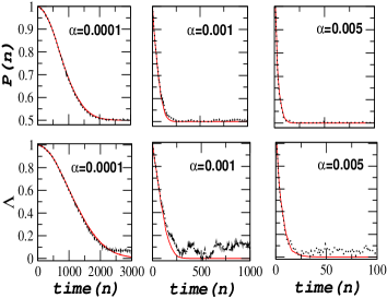
Figure 1: (Color online) Evolution of the system purity $P(n)$, and the parameter $\Lambda$ determines the entanglement in the system are plotted for three different system-environment coupling strengths $\alpha=0.0001,0.001,0.005$. Here the initial state is the Bell state (see the text). The dotted line is the exact numerical calculation, whereas the solid line is the theoretical estimation. We estimate $P(n)$ and $\Lambda$ from the approximate formula of the RDM $\rho_{S}$ of the system given in Eq. (Quantum chaotic system as a model of decohering environment).

Fig. 1 presents the result for the Bell state case. In the computational basis, diagonal elements of the initial density matrix $\rho_{S}(0)$ are $(1/2,0,0,1/2)$, and two off-diagonal elements have non-zero values : $\langle 00|\rho_{S}(0)|11\rangle=\langle 11|\rho_{S}(0)|00\rangle=-1/2$. These off-diagonal elements are not the part of the degenerate subspace, and therefore they decay in time. So in the asymptotic limit : $\rho_{S}\simeq\mbox{diag}\,(1/2,0,0,1/2)$, the purity $P$ and $\Lambda$ of this RDM are $1/2$ and $0$, respectively. In Fig. 1, we see that the purity $P$ and $\Lambda$ have reached very close to these asymptotic values. The rate, at which these two quantities have reached the asymptotic values, is determined by the coupling strength $\alpha$. As expected, for weaker coupling the rate is slower than stronger coupling. The most important fact is that our approximate formula for the RDM derived from the perturbation theory, is not only working well for the weak coupling case but also agrees very well for the stronger coupling cases.

Fig. 2 presents the result for the product state case. Initially $\Lambda=0$, and then it becomes negative till $n=1142$ for $\alpha=0.0001$, $n=81$ for $\alpha=0.001$, and $n=4$ for $\alpha=0.005$. Upto this time, entanglement between two qubits determined by the concurrence was zero. After that, there is a time interval when $\Lambda>0$, and the two qubits become entangled due to their common interaction with the chaotic environment. This shows that, like many-body environment [18], quantum chaotic environment can also generate entanglement between two non-interacting qubits which have no entanglement initially. In the asymptotic limit, diagonal elements of $\rho_{S}$ : $(1/4,1/4,-1/4,-1.4)$, and the off-diagonal elements : $\langle 01|\rho_{S}|10\rangle=\langle 10|\rho_{S}|01\rangle=-1/4$ corresponding to the degenerate subspace, survive from decoherence. Therefore, in this limit, the purity $P=3/8=0.375$, and $\Lambda=0$. Figure shows again a good agreement between the numerics and the theory.

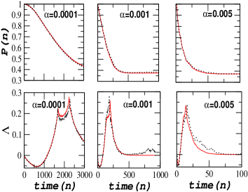
Figure 2: (Color online) Evolution of $P(n)$ and $\Lambda$ are plotted. Here initial state is the product state. Other parameters and descriptions are same as in Fig. 1.

Our theoretical formulation establishes the equivalence between quantum chaotic environment and many-body environment by showing the equivalence between their decoherence function $f(n)$. Therefore, it is very important to investigate $f(n)$ of the kicked top carefully. In Fig. 3, we plot the evolution of the decoherence function of the kicked top. Our numerical experiment suggests that the phenomenological formula for $f(n)$ given in Eq. (7) is not an exact formula for all time $n$. It describes short time quadratic and long time linear behavior well. So instead of fitting the numerics by the phenomenological formula, we interpolate it with a simple function $f(n)=an+bn^{2}$, a combination of a linear and a quadratic term. The interpolation (solid line of Fig. 3) gives $a\simeq 0.1776$ and $b\simeq 1.1561\times 10^{-3}$. We expect the parameter $a$ to be equal to the coefficient of the linear term of Eq. (7), i.e. $\frac{1}{2}C_{0}\coth(\gamma/2)$. For the chaotic kicked top, $C_{0}=\bigl{\langle}J_{z}(l)^{2}\bigr{\rangle}-\bigl{\langle}J_{z}(l)\bigr{\rangle}^{2}\simeq 1/3$. In addition, in strong chaos regime, the parameter $\gamma$ is very large which leads to $\coth(\gamma/2)\simeq 1$. Hence, the coefficient of the linear term of Eq. (7) is approximately equal to $1/6$, which is very close to the value obtained for the parameter $a$, i.e., $a\simeq 0.1776$. Thus we show that the decoherence function of the chaotic kicked top has the properties which are similar to the properties of any other model of decohering environment.

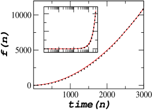
Figure 3: (Color online) Evolution of the decoherence function $f(n)$ of the kicked top. The dotted line is the exact numerics, and the solid line is the theoretical estimation. Inset is showing the same in semi-logarithmic scale, where the time-axis is in logarithmic scale.

In conclusion, as a model of decohering environment, we establish the equivalence between quantum chaotic system and any other many-body systems. This is an important result, which suggests that instead of complex many-body system one can use a simple chaotic system as a model of environment. Consequently, analytical investigations of environment induced decoherence would be easier, and from numerical point of view as well, this simple model requires very less computational resources. We substantiate our analytical formulation with strong numerical evidences. These show that quantum chaotic system is good decoherer, and it can also create entanglement between two non-interacting particles. The later result is very important due to the recent identification of entanglement as a resource for quantum computational and informational protocols [2].

We thank Drs. A. Tanaka, D. Cohen, and A. Lakshminarayan for useful comments and discussions.

References

- [1] W. H. Zurek, Rev. Mod. Phys 75, 715 (2003); E. Joos et al, Decoherence and the Appearance of a Classical World in Quantum Theory (2nd Ed., Springer, Berlin, 2003).
- [2] Any book on quantum computation. For example : M. A. Nielsen and I. L. Chuang, Quantum Computation and Quantum Information (Cambridge University Press, Cambridge, 2000).
- [3] R. P. Feynman and F. L. Vernon, Ann. Phys. 24, 118 (1963); A. O. Caldeira and A. J. Leggett, Ann. Phys. 149, 374 (1983).
- [4] A. J. Legget et. al., Rev. Mod. Phys. 59, 1 (1987).
- [5] J. Lages et al, Phys. Rev. E 72, 026225 (2005). A more recent paper : A. Relaño, J. Dukelsky, and R. A. Molina, Phys. Rev. E 76, 046223 (2007).
- [6] P. A. Mello, P. Pereyra, and N. Kumar, J. Stat. Phys. 51, 77 (1988); P. Pereyra, ibid 65, 773 (1991); M. Esposito and P. Gaspard, Phys. Rev. E 68, 066112 (2003); Phys. Rev. E 68, 066113 (2003); T. Gorin and T. H. Seligman, J. Opt. B 4, S386 (2002).
- [7] C. Pineda and T. H. Seligman, Phys. Rev. A 75, 012106 (2007); C. Pineda, T. Gorin, and T. H. Seligman, New J. Phys. 9, 106 (2007).
- [8] H. Kubotani, T. Okamura, and M. Sakagami, Physica A 214, 560 (1995); D. Cohen, Phys. Rev. Lett. 82, 4951 (1999); Phys. Rev. E 65, 026218 (2002); D. Cohen and T. Kottos, Phys. Rev. E 69, 055201(R) (2004).
- [9] D. Rossini, G. Benenti, and G. Casati, Phys. Rev. E 74, 036209 (2006).
- [10] D. Braun, F. Haake, and W. T. Strunz, Phys. Rev. Lett. 86, 2913 (2001).
- [11] F. Haake, Quantum Signatures of Chaos, 2nd Ed. (Springer-Verlag, Berlin, 2001).
- [12] S. Hill and W. K. Wootters, Phys. Rev. Lett. 78, 5022 (1997); W. K. Wootters, ibid. 80, 2245 (1998).
- [13] A. Tanaka, H. Fujisaki, and T. Miyadera, Phys. Rev. E 66, 045201(R) (2002). See also : H. Fujisaki, T. Miyadera, and A. Tanaka, Phys. Rev. E 67, 066201 (2003).
- [14] T. Prosen and T. H. Seligman, J. Phys. A 35, 4707 (2002). See also Ref. [7].
- [15] H. -J. Stöckmann and H. Kohler, Phys. Rev. E 73, 066212 (2006).
- [16] R. Schäfer et al, Phys. Rev. Lett. 95, 184102 (2005).
- [17] See particularly, Eq. (3) of Ref. [10].
- [18] D. Braun, Phys. Rev. Lett. 89, 277901 (2002).