Geometric extension of put-call symmetry in the multiasset setting

Abstract

In this paper we show how to relate European call and put options on multiple assets to certain convex bodies called lift zonoids. Based on this, geometric properties can be translated into economic statements and vice versa. For instance, the European call-put parity corresponds to the central symmetry property, while the concept of dual markets can be explained by reflection with respect to a plane. It is known that the classical univariate log-normal model belongs to a large class of distributions with an extra property, analytically known as put-call symmetry. The geometric interpretation of this symmetry property motivates a natural multivariate extension. The financial meaning of this extension is explained, the asset price distributions that have this property are characterised and their further properties explored. It is also shown how to relate some multivariate asymmetric distributions to symmetric ones by a power transformation that is useful to adjust for carrying costs. A particular attention is devoted to the case of asset prices driven by Lévy processes. Based on this, semi-static hedging techniques for multiasset barrier options are suggested.

Keywords: barrier option; convex body; dual market; Lévy process; lift zonoid; multiasset option; put-call symmetry; self-dual distribution; semi-static hedging

AMS Classifications: 60D05; 60E05; 60G51; 91B28; 91B70

1 Options and zonoids: an introduction

The stop-loss transformation from mathematical insurance theory associates a random variable $\zeta$ with its stop-loss $\mathbf{E}(\zeta-k)_{+}$ at level $k$. Here $\mathbf{E}$ denotes the expectation and $x_{+}=\max(x,0)$ for a real number $x$, where $k$ is usually interpreted as the excess (part of claim which is not paid by the insurer).

From the mathematical finance viewpoint, the stop-loss transformation is identified as the expected payoff from a European call option for $\zeta=S_{T}=S_{0}e^{rT}\eta$ being the price of a (say non-dividend paying) asset at the maturity time $T$, where $S_{0}$ is the spot price and $e^{rT}\eta$ is the factor by which the price changes, $r$ is the (constant) risk-free interest rate and $\eta$ is an almost surely positive random variable. In arbitrage-free and complete markets the expectation can be taken with respect to the unique equivalent martingale measure, so that the expected value of the discounted payoff becomes the call price. If the underlying probability measure is a martingale measure, then $\mathbf{E}\eta=1$ and the discounted price process $S_{t}e^{-rt}$, $t\in[0,T]$, becomes a martingale. Unless indicated by a different subscript, all expectations in this paper are understood with respect to the probability measure $\mathbf{Q}$, which is not necessarily a martingale measure. In this paper we do not address the choice of a martingale measure in incomplete markets.

The expected call payoff $\mathbf{E}(S_{T}-k)_{+}$ can be considered a function of the bivariate vector $(k,F)$, where

$$F=S_{0}e^{rT}$$

is the theoretical forward price on the same asset with the same maturity, i.e. $\mathbf{E}(S_{T}-k)_{+}=\mathbf{E}(F\eta-k)_{+}$. Deterministic dividends or income until maturity can be incorporated in the forward price, e.g. by setting $F=S_{0}e^{(r-q)T}$ in case of a continuous dividend yield $q$.

When working with $n$ assets, we write $\eta$ for an $n$-dimensional random vector $(\eta_{1},\dots,\eta_{n})$ such that the price $S_{Ti}$ of the $i$th asset at time $T$ equals $F_{i}\eta_{i}$ with $F_{i}$ being the corresponding forward price. We denote this shortly as

$$S_{T}=F\circ\eta=(F_{1}\eta_{1},\dots,F_{n}\eta_{n})\,.$$ (1.1)

In order to relate the expected payoffs to certain convex sets we need the following basic concept from convex geometry.

Definition 1.1 (see [36], Sec. 1.7).

The support function of a nonempty convex compact set $K$ in the $n$-dimensional Euclidean space $\mathbb{R}^{n}$ is defined by

$$h_{K}(u)=\sup\{\langle x,u\rangle:\;x\in K\}\,,\quad u\in\mathbb{R}^{n}\,,$$

where $\langle x,u\rangle$ is the scalar product in $\mathbb{R}^{n}$.

For instance, if $K=[-x,x]$ is the line segment in $\mathbb{R}^{n}$ with end-points $\pm x$, then $h_{K}(u)=|\langle x,u\rangle|$; if $K=[0,x]$, then $h_{K}(u)=\langle x,u\rangle_{+}$; if $K$ is the triangle in $\mathbb{R}^{2}$ with vertices $(0,0)$, $(a,0)$, and $(0,b)$, then $h_{K}(u)=\max(u_{1}a,u_{2}b,0)$ for all $u=(u_{1},u_{2})\in\mathbb{R}^{2}$.

A function $g:\mathbb{R}^{n}\mapsto\mathbb{R}$ is called sublinear if it is positively homogeneous ($g(cx)=cg(x)$ for all $c\geq 0$ and $x\in\mathbb{R}^{n}$) and subadditive ($g(x+y)\leq g(x)+g(y)$ for all $x,y\in\mathbb{R}^{n}$). It is well known in convex geometry that support functions are characterised by their sublinearity property and that there is a one-to-one correspondence between support functions and convex bodies, i.e. nonempty compact convex subsets of $\mathbb{R}^{n}$, see e.g. [36, Th. 1.7.1].

With each integrable $n$-dimensional random vector $\eta=(\eta_{1},\dots,\eta_{n})$ it is possible to associate a $(n+1)$-dimensional convex body which uniquely describes the distribution of $\eta$. For this, consider $(n+1)$-dimensional random vector $(1,\eta)$ obtained by concatenating $1$ and $\eta$ or, in other words, by lifting $\eta$ with an extra coordinate being one. In the financial setting this extra coordinate represents a riskless bond. Because of the lifting, we number the coordinates of $(n+1)$-dimensional vectors as $0,1,\dots,n$ and write these vectors as $(u_{0},u)$ for $u_{0}\in\mathbb{R}$ and $u\in\mathbb{R}^{n}$ or as $(u_{0},u_{1},\dots,u_{n})$.

Let $X$ be the random set being the line segment in $\mathbb{R}^{n+1}$ with end-points at the origin and $(1,\eta)$, see [26] for detail presentation of random sets theory. The support function of $X$ is given by

$$h_{X}(u_{0},u)=\max(u_{0}+u_{1}\eta_{1}+\cdots+u_{n}\eta_{n},0)=\langle(u_{0},u),(1,\eta)\rangle_{+}$$

for $(u_{0},u)\in\mathbb{R}^{n+1}$. The integrability of $\eta$ implies that $h_{X}(u_{0},u)$ is integrable. The expected support function $\mathbf{E}h_{X}$ is sublinear and so is the support function of a convex body $\mathbf{E}X$ called the (Aumann) expectation of $X$, see [26, Sec. 2.1]. For our choice of $X$, the set $\mathbf{E}X$ is called the lift zonoid of $\eta$ and denoted by $Z_{\eta}$. It is known that $Z_{\eta}$ determines uniquely the distribution of $\eta$, see [29, Th. 2.21]. Note that the zonoid of $\eta$ appears from a similar (non-lifted) construction as the expectation of the random segment that joins the origin and $\eta$, see [29, Th. 2.8].

In the univariate setting we assume that $n=1$ and $\eta=S_{T}/F$ is a positive random variable. Then

$$h_{Z_{\eta}}(u_{0},u_{1})=\mathbf{E}(u_{0}+u_{1}\eta)_{+}=\begin{cases}u_{0}+u_{1}\mathbf{E}\eta&u_{0},u_{1}\geq 0\,,\\ 0&u_{0},u_{1}<0\,,\\ \mathbf{E}(u_{0}+u_{1}\eta)_{+}&\text{otherwise }\end{cases}$$ (1.2)

for all $(u_{0},u_{1})\in\mathbb{R}^{2}$. Figure 1 shows the lift zonoid of $\eta$ for various volatilities ($0.25,0.5,0.75$) in the log-normal case with $\mathbf{E}\eta=1$ calculated for $T=1$. The higher the volatility the larger (thicker) becomes the lift zonoid. The upper and lower boundaries of lift zonoids are the so-called generalised Lorenz curves, which can be easily parametrised, see [29, pp. 43 and 44].

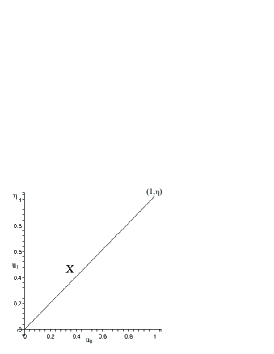
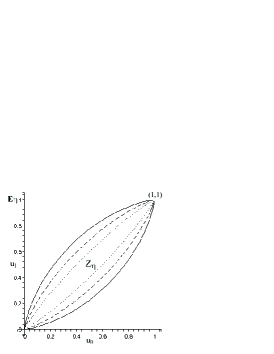
Figure 1: The segment $X=[(0,0),(1,\eta)]$ and the lift zonoid $Z_{\eta}$ for log-normal $\eta$ with volatilities $\sigma=0.25,0.5,0.75$, drift $\mu=-\frac{1}{2}\,\sigma^{2}$ and maturity $T=1$.

Since the lift zonoid uniquely determines the distribution of random vector $\eta=(\eta_{1},\dots,\eta_{n})$, it also determines prices of all payoffs associated with $S_{T}=(S_{T1},\dots,S_{Tn})$, assuming that the underlying probability measure is a martingale measure. For instance, in the univariate case $h_{Z_{\eta}}(-k,F)$ (resp. $h_{Z_{\eta}}(k,-F)$) is the non-discounted price of a European call (resp. put) option with strike $k$. A similar interpretation holds for basket options. The support function determines uniquely the lift zonoid, so that the prices of European vanilla options (basket calls and puts) determine uniquely the distribution of the assets and so prices of all other European options. In the univariate case this fact was noticed by Ross [31], Breeden and Litzenberger [5], while Carr and Madan [12] presented an explicit decomposition of general smooth payoff functions as integrals of vanilla options and riskless bonds. In view of the positive homogeneity of support functions and central symmetry of lift zonoids, see [29, Prop. 2.15], it suffices in fact to have all call prices with parameter vectors $(-k,u)$ with norm one in $\mathbb{R}^{n+1}$, where $k>0$ and $u$ stands for the vector containing the products of the weights and forward prices of the corresponding assets in the components. Alternatively, it suffices to have all call prices for any fixed $k>0$ and any $u\in\mathbb{R}^{n}$.

As just mentioned it is well known that the lift zonoid is centrally symmetric. Section 2 begins by showing that the central symmetry property of lift zonoids is a geometric interpretation of the call-put parity for European options.

The main question addressed in this paper concerns further symmetry properties of lift zonoids, their probabilistic characterisation and financial implications. Section 2 continues to show that in the univariate case (where lift zonoids are planar sets) the reflection at the line bisecting the first quadrant corresponds to the dual market transition at maturity. In view of this, random variables that lead to line symmetric lift zonoids are called self-dual. This property has an immediate financial interpretation as Bates’ rule [4] or the put-call symmetry [6, 10]. For instance, the lift zonoids of the log-normal distribution in the risk-neutral setting (see Figure 1) are line symmetric, which implies the put-call symmetry (or Bates’ rule) for the Black-Scholes economy. Section 2 then shows how to translate the geometric symmetry property into symmetry relationships for general integrable payoffs and, in particular, for various binary and gap options.

Section 3 highlights relationships between vanilla options and options on the maximum of the asset price and a strike. This leads to a concept of lift max-zonoids, which are particularly useful to describe options involving maxima of possibly weighted assets. This section also deals with a symmetry property of lift max-zonoids and shows how to relate option prices to certain norms on $\mathbb{R}^{2}$ yielding a relationship to the extreme values theory.

Section 4 characterises random vectors that possess symmetry properties generalising the classical put-call symmetry for basket options and options on the maximum of several assets. The symmetry (or self-duality) is understood with respect to each particular asset or for all assets simultaneously. Relationships between the self-duality property and the swap-invariance in Margrabe type options have been studied in [28]. In currency markets, the self-duality results can be interpreted with respect to real existing markets, yielding the basis for further applications, see [35]. The overall symmetry implies that expected payoffs from basket options are symmetric with respect to the weights of particular assets and the strike price. We show that symmetries for some vanilla type options (like Bates’ rule in the univariate case) imply a certain symmetry for every integrable payoff function. After discussing some fundamental results, we characterise the multivariate log-infinitely divisible distributions, exhibiting the multivariate put-call symmetry. The new effect in the multivariate setting is that independence of asset prices prevents them from being jointly self-dual. In other words, symmetry properties for several assets enforce certain dependency structure between them, which is explored in this paper.

In order to extend the application range of the self-duality property and also in view of incorporating the carrying costs, we then define quasi-self-dual random vectors and characterise their distributions. These random vectors become self-dual if their components are normalised by constants (representing carrying costs) and raised to a certain power. The related power transformation was used in [11, Sec. 6.2] in the one-dimensional case. Here we establish an explicit relationship between carrying costs and the required power of transformation for rather general price models based on Lévy processes.

These results are then used in Section 5 to obtain several new results for self-dual random variables thereby complementing the results from [11]. In particular, self-dual random variables have been characterised in terms of their distribution functions; it is shown that self-dual random variables always have non-negative skewness and several examples of self-dual random variables are given.

As in the univariate case also in the multiasset case there are various applications of symmetry results. First, symmetry results may be used for validating models or analysing market data, e.g. similarly as in [4] and [17] in the univariate case. Furthermore, they could be used for deriving certain investment strategies, see e.g. Section 6.4. The probably most important application will potentially be found in the area of hedging, especially in developing semi-static replicating strategies of multiasset barrier and possibly also more complicated path-dependent contracts. Following Carr and Lee [11], semi-static hedging is the replication of contracts by trading European-style claims at no more than two times after inception. As far as the relevance of this application is concerned we should mention that there has been a liquid market in structured products, particularly in Europe. At the moment the majority of the trades is still over-the-counter, but more and more trades are also organised at exchanges, especially at the quite new European exchange for structured products Scoach. Structured products often involve equity indices, sometimes several purpose-built shares, and quite often have barriers. Hence, developing robust hedging strategies for multi-asset path-dependent products seems to be of a certain importance. In the univariate case, Carr et al. [8, 9, 10, 11] and several other authors (see e.g. [2, 1, 30]) developed a machinery for replicating barrier contracts having fundamental relevance for other path-dependent contracts.

Section 6 contains first applications of the multivariate symmetry properties, especially for hedging complex barrier options, thereby extending results from [8, 9, 10] and [11] for some multiasset options. The development of a more general multivariate semi-static hedging machinery is left for future research.

2 Symmetries of lift zonoids and financial relations for a single asset case

2.1 Parities

We write $c(k,F)$ for the price of the European call option with strike $k$ on the asset with forward price $F$. Furthermore, let $p(k,F)$ denote the price of the equally specified put. The maturity time $T$ is supposed to be the same for all instruments.

One of the most basic relationships between options in arbitrage-free markets is the European call-put parity. In case of deterministic dividends, this parity can be expressed by

$$c(k,F)=e^{-rT}(F-k)+p(k,F)\,.$$ (2.1)

Recall that $\eta$ is defined by $S_{T}=F\eta$, where $S_{T}$ is the asset price at maturity and $F$ is the forward price. The lift zonoid $Z_{\eta}$ of $\eta$ is centrally symmetric around $\frac{1}{2}\,(1,\mathbf{E}\eta)$, see [29, Prop. 2.15]. If the expectation is taken with respect to a martingale measure, then $\mathbf{E}\eta=1$, whence $Z_{\eta,o}=Z_{\eta}-(\frac{1}{2}\,,\frac{1}{2}\,)$ is origin symmetric, so that $h_{Z_{\eta,o}}(u)=h_{Z_{\eta,o}}(-u)$ for all $u\in\mathbb{R}^{2}$. Interpreting the values of the support function of $Z_{\eta}$ as non-discounted call and put prices, this symmetry yields that

$$e^{rT}c(k,F) =h_{Z_{\eta}}(-k,F)=h_{Z_{\eta,o}+(\frac{1}{2}\,,\frac{1}{2}\,)}(-k,F)$$

$$=h_{Z_{\eta,o}}(k,-F)-\frac{1}{2}\,k+\frac{1}{2}\,F$$

$$=h_{Z_{\eta,o}}(k,-F)+\frac{1}{2}\,k-\frac{1}{2}\,F-k+F$$

$$=h_{Z_{\eta}}(k,-F)-k+F=e^{rT}p(k,F)+F-k\,,$$

i.e. we arrive at the classical European call-put parity. By defining appropriate multidimensional lift zonoids and using their point symmetry, the above proof can easily be extended to the call-put parity for Asian options with arithmetic mean and to the European call-put parity for basket options.

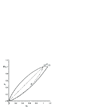
Figure 2: An approximation of the payoff set $A$ for the Black-Scholes economy with volatility $\sigma=0.5$, interest rate $r=0.12$, dividend yield $q=0$ and maturity $T=1$.

It is also easy to explain geometrically why the parities do not hold for American options. Let $C(k,F)$ (resp. $P(k,F)$) be the price of an American call (resp. put) with strike $k$ on the asset with forward price $F$. Since the functions $C$ and $P$ are sublinear, it is possible to define convex body $A$ with support function $h_{A}(-k,F)=e^{rT}C(k,F)$ and $h_{A}(k,-F)=e^{rT}P(k,F)$, for $k,F>0$. This convex body (that we call a payoff set) determines the values of American vanilla options and is, up to some rare exceptions, not centrally symmetric, see Figure 2.

2.2 Duality

Recall that $\eta$ defined from $S_{T}=F\eta$ is almost surely positive. If $\eta$ is distributed according to a martingale measure $\mathbf{Q}$, then a new probability measure $\tilde{\mathbf{Q}}$ can be defined from

$$\frac{d\tilde{\mathbf{Q}}}{d\mathbf{Q}}=\eta\,.$$

Since $\eta$ is usually represented as $e^{H_{T}}$ for a semimartingale $H_{t}$, $0\leq t\leq T$, and $-H_{t}$ is called the dual to $H_{t}$, the random variable $\tilde{\eta}=\eta^{-1}$ is said to be the dual of $\eta$. The dual lift zonoid $Z_{\tilde{\eta}}$ is defined as the $\tilde{\mathbf{Q}}$-expectation of the segment that joins the origin and $(1,\tilde{\eta})$.

Lemma 2.1.

If $Z_{\eta}$ is the lift zonoid generated by almost surely positive random variable $\eta$ with $\mathbf{E}\eta=1$, then

$$Z_{\tilde{\eta}}=\tilde{Z}_{\eta}\,,$$

where $\tilde{Z}_{\eta}$ denotes the reflection of $Z_{\eta}$ with respect to the line $\{(u_{0},u_{1})\in\mathbb{R}^{2}:\;u_{0}=u_{1}\}$.

Proof.

For $(u_{0},u_{1})\in\mathbb{R}^{2}$

$$h_{Z_{\tilde{\eta}}}(u_{0},u_{1}) =\mathbf{E}_{\tilde{\mathbf{Q}}}(u_{0}+u_{1}\tilde{\eta})_{+}=\mathbf{E}\big{[}(u_{0}+u_{1}\eta^{-1})_{+}\eta\big{]}$$

$$=h_{Z_{\eta}}(u_{1},u_{0})=h_{\tilde{Z}_{\eta}}(u_{0},u_{1})\,.$$

noticing that the support function of $\tilde{Z}_{\eta}$ is obtained from the support function of $Z_{\eta}$ by swapping the coordinates. ∎

Since $Z_{\eta}$ is centrally symmetric with respect to $(\frac{1}{2}\,,\frac{1}{2}\,)$, the set $\tilde{Z}_{\eta}$ can also be obtained by reflecting $Z_{\eta}$ with respect to the line $\{(u_{0},u_{1}):\;u_{1}=1-u_{0}\}$.

Lemma 2.1 relates the symmetry property of lift zonoids to the duality principle in option pricing at maturity. This principle traces its roots to observations by Merton [25], Grabbe [20], McDonald and Schroder [24], Bates [3], and Carr [6] and has been studied extensively over the recent years, e.g. Carr and Chesney [7] and Detemple [14] discuss American version of duality. For a detailed presentation of the duality principle in a general exponential semimartingale setting and for its various applications see Eberlein et al. [15] and the literature cited therein. The multiasset case has been studied in Eberlein et al. [16].

Consider a European call option valued at $c(k,F,\mathbf{Q})$ with strike $k$ and maturity $T$ on a share represented in a risk-neutral world by a $\mathbf{Q}$-price process $S_{t}=S_{0}e^{(r-q)t}\eta_{t}=F_{t}\eta_{t}$, i.e. the share is traded in a market with deterministic risk-free interest rate $r$ and attracts deterministic dividend-yield $q$, while $\eta_{t}$ is a $\mathbf{Q}$-martingale. In the most common setting this call option is related to a dual European put $\tilde{p}(S_{0},\tilde{F},\tilde{\mathbf{Q}})$ with strike $S_{0}$ and the same maturity $T$ on a share represented by the dual $\tilde{\mathbf{Q}}$-price process $\tilde{S}_{t}=ke^{(q-r)t}\tilde{\eta}_{t}=\tilde{F}_{t}\tilde{\eta}_{t}$, where $\tilde{\eta}_{t}$ is a $\tilde{\mathbf{Q}}$-martingale. In other words, the dual put is written on another (dual) share traded in the dual market with risk-free interest rate $q$ assuming that this dual share attracts dividend-yield $r$. By Lemma 2.1 we get the following geometric proof and interpretation of the European call-put duality,

$$\tilde{p}(S_{0},\tilde{F},\tilde{\mathbf{Q}}) =e^{-qT}\mathbf{E}_{\tilde{\mathbf{Q}}}(S_{0}-\tilde{F}\tilde{\eta})_{+}=e^{-qT}h_{Z_{\tilde{\eta}}}(S_{0},-\tilde{F})$$

$$=e^{-qT}h_{\tilde{Z}_{\eta}}(S_{0},-\tilde{F})$$

$$=e^{-qT}h_{Z_{\eta}}(-\tilde{F},S_{0})=e^{-qT}\mathbf{E}_{\mathbf{Q}}(S_{0}\eta-\tilde{F})_{+}$$

$$=e^{-rT}\mathbf{E}_{\mathbf{Q}}(S_{0}e^{(r-q)T}\eta-ke^{(q-r)T+(r-q)T})_{+}=c(k,F,\mathbf{Q})\,.$$

By the classical call-put parity, a call-call duality can be derived in a straightforward way. The duality for American options (see [7, 14, 37]) can be interpreted geometrically by reflecting the payoff set $A$ (see Figure 2) at the line bisecting the first quadrant.

2.3 Symmetries for vanilla options

If $Z_{\eta}$ is symmetric with respect to the line $\{(u_{0},u_{1}):\;u_{0}=u_{1}\}$ bisecting the first quadrant, i.e.

$$\tilde{Z}_{\eta}=Z_{\eta}\,,$$ (2.2)

the duality relates out-of-the-money to certain in-the-money calls in the same market. We call a positive random variable $\eta$ self-dual if (2.2) holds. This symmetry property (2.2) clearly depends on the probability measure used to define the expectation. It implies that $\mathbf{E}\eta=1$, i.e. in the one period setting each probability measure that makes $\eta$ self-dual is a martingale measure.

Theorem 2.2.

Assume that the asset price at maturity of an asset with deterministic dividend payments is $S_{T}=F\eta$ with self-dual $\eta$. Then

$$e^{rT}c(k,F)+k=e^{rT}c(F,k)+F\,.$$ (2.3)

Proof.

Noticing (2.2), we have

$$e^{rT}c(k,F)=h_{Z_{\eta}}(-k,F)=h_{\tilde{Z}_{\eta}}(F,-k)=h_{Z_{\eta}}(F,-k)=e^{rT}p(F,k)\,.$$

The proof is finished by applying the put-call parity. ∎

Since $c(k,F)$ is positively homogeneous in both arguments, i.e. $c(tk,tF)=tc(k,F)$ for $t\geq 0$, the symmetry relation (2.3) can also be written as

$$\frac{\tilde{c}(m)+e^{-rT}}{\tilde{c}(m^{-1})+e^{-rT}}=m\,,$$

where $m=F/k$ determines the moneyness of the call and $\tilde{c}(m)=c(1,m)$.

Corollary 2.3.

Assuming (2.2), the following European symmetries hold

$$p(k,F) =c(F,k)\,,$$ (2.4)

$$e^{rT}p(k,F)+F =k+e^{rT}p(F,k)\,.$$ (2.5)

Proof.

By (2.3) and (2.1) we obtain

$$c(F,k)=c(k,F)-Fe^{-rT}+ke^{-rT}=p(k,F)\,.$$

By combining the left-hand side of (2.3) with (2.4) for the reversed order of $k$ and $F$ and the right-hand side of (2.3) with (2.4) we arrive at (2.5). ∎

The above relations are known in the literature as put-call symmetry, see e.g. [4], [6], [10], and more recently [17, 18] for log-infinitely-divisible models, which are further discussed in Section 4.3. Further recent developments are presented in [11]. There are various applications of the put-call symmetry, especially in connection with hedging exotic options, see [10, 11] and Section 6.

2.4 General symmetry

The following result obtained in [11, Th. 2.2] (without use of lift zonoids) generalises the self-duality to a wide range of payoff functions.

Theorem 2.4.

An integrable random variable $\eta$ is self-dual if and only if for any payoff function $f:\mathbb{R}_{+}\mapsto\mathbb{R}$ such that $\mathbf{E}|f(F\eta)|<\infty$ for $F>0$,

$$\mathbf{E}f(F\eta)=\mathbf{E}[f(F\eta^{-1})\eta]\,.$$ (2.6)

Proof.

Changing measure from $\mathbf{Q}$ to its dual $\tilde{\mathbf{Q}}$, we arrive at

$$\mathbf{E}_{\mathbf{Q}}f(F\eta)=\mathbf{E}_{\tilde{\mathbf{Q}}}[f(F\eta)\eta^{-1}]=\mathbf{E}_{\tilde{\mathbf{Q}}}[f(F\tilde{\eta}^{-1})\tilde{\eta}]\\ =\mathbf{E}_{\mathbf{Q}}[f(F\eta^{-1})\eta]\,.$$

Since lift zonoids uniquely determine distributions of random variables, the last equality holds by Lemma 2.1 in view of the symmetry assumption (2.2). Conversely, if (2.6) holds for any integrable payoff-function, then it holds for any vanilla options, i.e. $h_{Z_{\eta}}(-k,F)=h_{Z_{\eta}}(F,-k)=h_{\tilde{Z}_{\eta}}(-k,F)$ for every $k>0$, implying (2.2). ∎

Denote by $\operatorname{BC}(k_{c},F)$ and $\operatorname{GC}(k_{c},F)$ the arbitrage-free values of a binary call and gap call with maturity $T$ and strike $k_{c}$, i.e. the European derivatives with payoffs $\operatorname{{1I}}_{S_{T}>k_{c}}$ and $S_{T}\operatorname{{1I}}_{S_{T}>k_{c}}$. Furthermore, $\operatorname{BP}(k_{p},F)$ and $\operatorname{GP}(k_{p},F)$ denote the arbitrage-free values of the equally specified puts, i.e. the European derivatives with payoffs $\operatorname{{1I}}_{S_{T}<k_{p}}$ and $S_{T}\operatorname{{1I}}_{S_{T}<k_{p}}$. Theorem 2.4 yields the following result, which is equivalent to [11, Cor. 2.9] being a generalisation of the binary put-call symmetry from [10].

Corollary 2.5.

Under the assumptions of Theorem 2.4 the following relationships hold:

$$\sqrt{k_{c}}\operatorname{BC}(k_{c},F)=\frac{1}{\sqrt{k_{p}}}\operatorname{GP}(k_{p},F),\qquad\sqrt{k_{p}}\operatorname{BP}(k_{p},F)=\frac{1}{\sqrt{k_{c}}}\operatorname{GC}(k_{c},F)\,,$$

where the forward price $F$ equals the geometric mean of the binary (resp. gap) call strike $k_{c}$ and the gap (resp. binary) put strike $k_{p}$, i.e. $F=\sqrt{k_{c}k_{p}}$.

Proof.

If $\sqrt{k_{c}k_{p}}=F$, then (2.6) yields that

$$e^{rT}\operatorname{BC}(k_{c},F) =\mathbf{E}[\operatorname{{1I}}_{F\eta>k_{c}}]=\mathbf{E}[\eta\operatorname{{1I}}_{F\eta^{-1}>k_{c}}]=\mathbf{E}\Big{[}\eta\frac{F}{\sqrt{k_{c}k_{p}}}\operatorname{{1I}}_{\sqrt{k_{c}k_{p}}>k_{c}\eta}\Big{]}$$

$$=\frac{1}{\sqrt{k_{c}k_{p}}}\mathbf{E}[S_{T}\operatorname{{1I}}_{k_{p}>S_{T}}]=\frac{e^{rT}}{\sqrt{k_{c}k_{p}}}\operatorname{GP}(k_{p},F)\,.$$

The proof of the second identity is similar. ∎

Thus, symmetry properties for particular options (vanilla, binary/gap, straddles, etc.) are nothing but writing down Equation (2.6) for special payoff functions.

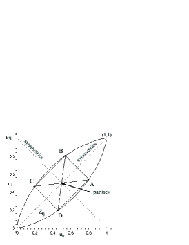
Figure 3: Symmetries of $Z_{\eta}$ for self-dual $\eta$ and their financial interpretations.

The random variable $\eta$ has no atoms if and only if the support function $h_{Z_{\eta}}$ is continuously differentiable on $\mathbb{R}^{2}\setminus\{0\}$, so that $Z_{\eta}$ is strictly convex, see [36, Sec. 2.5]. Then the unique point on the boundary of $Z_{\eta}$ (without the points $(0,0)$, $(1,1)$) at which $(u_{0},u_{1})\in\mathbb{R}^{2}\setminus\{0\}$ is the outward normal vector to $Z_{\eta}$ is given by

$$\operatorname{grad}h_{Z_{\eta}}(u_{0},u_{1})=\left(\frac{\partial h_{Z_{\eta}}}{\partial u_{0}},\frac{\partial h_{Z_{\eta}}}{\partial u_{1}}\right)\,.$$

Assuming that the underlying probability measure $\mathbf{Q}$ is a martingale measure and calculating the gradient of the support function $h_{Z_{\eta}}$ at $(u_{0},u_{1})=(-k,F)$ with $k,F>0$ yield another parametrisation of the upper boundary of $Z_{\eta}$ as

$$\operatorname{grad}h_{Z_{\eta}}(-k,F)=e^{rT}\left(\operatorname{BC}(k,F),\frac{\operatorname{GC}(k,F)}{F}\right),\quad k>0\,.$$

Analogously, the lower boundary is parametrised by

$$\operatorname{grad}h_{Z_{\eta}}(k,-F)=e^{rT}\left(\operatorname{BP}(k,F),\frac{\operatorname{GP}(k,F)}{F}\right),\quad k>0\,.$$

Hence, in non-atomic cases the boundaries of the lift zonoid $Z_{\eta}$ can be parametrised by non-discounted arbitrage-free values of binary and normalised gap options. Thus, the distribution of $\eta$ is also reflected in these pairs of options.

Figure 3 interprets financial parities and symmetries geometrically for the lift-zonoid $Z_{\eta}$. By comparing the coordinates of the points A, B, C, D we get relations between binary and gap options. By comparing the related values of the support function $h_{Z_{\eta}}$ we arrive at the put-call parity and symmetry for vanilla options. Combining A with C yields parities between certain in-the-money puts (vanilla, binary, and gap) and the related out-of-the-money calls. Connecting the points B and D yields the same parity results, except that B represents certain in-the-money calls and D the related out-of-the-money puts. Comparing C with D yields out-of-the-money put call symmetry results, while linking A with B leads to the same results for in-the-money options. Finally combining B with C (resp. A with D) results in the call-call (resp. put-put) symmetry.

3 Options on maximum and lift max-zonoids

Since the call payoff can be written as

$$(S_{T}-k)_{+}=\max(S_{T},k)-k\,,\quad S_{T},k\geq 0\,,$$ (3.1)

the expected call payoff can be related to another convex compact subset $M_{\eta}$ of $\mathbb{R}^{2}$ that has the support function

$$h_{M_{\eta}}(k,F)=\mathbf{E}\max(k,F\eta,0)\,,\quad(k,F)\in\mathbb{R}^{2}\,.$$ (3.2)

The set $M_{\eta}$ is defined as the Aumann expectation of the random triangle with vertices at the origin, $(1,0)$, and $(0,\eta)$. Because the financial quantities are non-negative, we often restrict the support function onto the first quadrant $\mathbb{R}_{+}^{2}$. Then it is possible to write (3.2) as

$$h_{M_{\eta}}(k,F)=\mathbf{E}\max(k,F\eta)\,,\quad(k,F)\in\mathbb{R}_{+}^{2}\,.$$ (3.3)

If $\eta=(\eta_{1},\dots,\eta_{n})$ is a random vector in $\mathbb{R}_{+}^{n}=[0,\infty)^{n}$, a similar to (3.2) construction leads to the set $M_{\eta}$ called the lift max-zonoid of $\eta$ and defined as the Aumann expectation of the random crosspolytope with vertices at the origin and the unit basis vectors $e_{0},e_{1},\dots,e_{n}$ in $\mathbb{R}^{n+1}$ scaled respectively by $1,\eta_{1},\dots,\eta_{n}$, i.e.

$$h_{M_{\eta}}(u_{0},u_{1},\dots,u_{n})=\mathbf{E}\max(0,u_{0},u_{1}\eta_{1},\dots,u_{n}\eta_{n})\,,(u_{0},u_{1},\dots,u_{n})\in\mathbb{R}^{n+1}\,.$$

Max-zonoids have been introduced in [27] in view of their use in extreme values theory. If $\mathbf{E}\eta=(1,\dots,1)$, then $M_{\eta}$ is a convex compact subset of the unit cube $[0,1]^{n+1}$ that contains the origin and all unit basis vectors. If $n=1$, then each such set is a lift max-zonoid of some random variable, while this no longer holds for two and more assets, see [27, Th. 2].

Theorem 3.1.

The lift max-zonoid $M_{\eta}$ of an integrable random vector $\eta\in\mathbb{R}_{+}^{n}$ determines uniquely the distribution of $\eta$.

Proof.

The support function $h_{M_{\eta}}(u_{0},u_{1},\dots,u_{n})$ for $u_{0},u_{1},\dots,u_{n}\geq 0$ can be written as $\mathbf{E}\max(u_{0},\zeta)$ for $\zeta=\max(u_{1}\eta_{1},\dots,u_{n}\eta_{n})$ and so determines uniquely the distribution of $\zeta$. The cumulative distribution function of $\zeta$ is given by

$$F_{\zeta}(t)=\mathbf{P}\{\eta_{1}\leq\frac{t}{u_{1}},\dots,\eta_{n}\leq\frac{t}{u_{n}}\}$$

and so determines uniquely the joint cumulative distribution function of $\eta_{1},\dots,\eta_{n}$. ∎

If the underlying probability measure is a martingale measure, Theorem 3.1 implies that prices of options on the maxima of weighted assets determine the joint distribution of the risky assets and so prices of all other payoffs. In view of the positive homogeneity of support functions it suffices that the expected values are known for parameter vectors $(u_{0},u)$ with norm one in $\mathbb{R}^{n+1}$, $u_{0}>0$ and $u$ with strictly positive coordinates. Alternatively, it suffices to know the expected values for fixed $u_{0}>0$ and $u$ with strictly positive coordinates.

The remainder of this section deals with the single asset case. Equation (3.1) suggests that in this case, the lift max-zonoid is closely related to the lift zonoid $Z_{\eta}$ of a random variable $\eta$.

Lemma 3.2.

If $M_{\eta}$ is the lift max-zonoid generated by a non-negative integrable random variable $\eta$, then

$$M_{\eta}=\operatorname{conv}\{(0,0)\cup(Z^{\prime}_{\eta}+(1,0))\}\,,$$

where $Z^{\prime}_{\eta}$ is the reflection of $Z_{\eta}$ with respect to the line $\{(u_{0},u_{1}):\;u_{0}=0\}$ and $\operatorname{conv}$ denotes the convex hull, see Figure 4.

Proof.

For $(u_{0},u_{1})\in\mathbb{R}^{2}$ the support function of the set in the right-hand side is given by

$$\max(0,h_{Z^{\prime}_{\eta}}(u_{0},u_{1})+u_{0}) =\max(0,h_{Z_{\eta}}(-u_{0},u_{1})+u_{0})$$

$$=\max(0,\mathbf{E}(u_{1}\eta-u_{0})_{+}+u_{0})\,.$$

By checking all possible signs of $u_{0}$ and $u_{1}$ it is easy to see that this support function equals $\mathbf{E}\max(0,u_{0},u_{1}\eta)=h_{M_{\eta}}(u_{0},u_{1})$. ∎

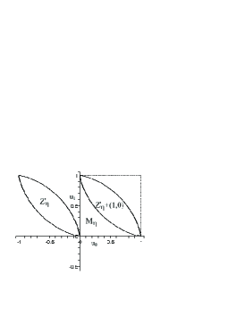
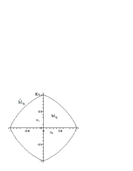
Figure 4: Relation between $M_{\eta}$ and $Z_{\eta}$ as well as the body $\hat{M}_{\eta}$ for log-normal $\eta$ with mean one and volatility $\sigma=0.5$ calculated for $T=1$.

Lemma 3.2 implies that the duality transform from Section 2.2 amounts to the symmetry of $M_{\eta}$ with respect to the line bisecting the first quadrant. Furthermore, $\eta$ is self-dual if and only if $M_{\eta}$ is symmetric with respect to this line, i.e.

$$\mathbf{E}\max(F\eta,k)=\mathbf{E}\max(F,k\eta)\,,\quad k,F\geq 0\,.$$ (3.4)

Indeed, since

$$h_{Z_{\eta}}(-u_{0},u_{1}) =\mathbf{E}\max(u_{1}\eta,u_{0})-u_{0}\,,$$

$$h_{Z_{\eta}}(u_{1},-u_{0}) =\mathbf{E}\max(u_{1},u_{0}\eta)-u_{0}\,,$$

for $u_{0},u_{1}\geq 0$, the symmetry property (2.2) is equivalent to (3.4).

The Euclidean space $\mathbb{R}^{2}$ can be equipped with various norms. Each norm on $\mathbb{R}^{2}$ can be described as the support function of a centrally symmetric (with respect to the origin) convex body that contains the origin in its interior. Although $M_{\eta}$ in Lemma 3.2 is a subset of $\mathbb{R}_{+}^{2}$ and so does not contain the origin in its interior, it is possible to use $h_{M_{\eta}}$ to define the norm on the whole plane as

$$\|x\|_{\eta}=h_{M_{\eta}}(|x|)=h_{\hat{M}_{\eta}}(x)\,,$$

where $|x|$ is the vector composed of the absolute values of the components of $x\in\mathbb{R}^{2}$ and $\hat{M}_{\eta}$ is obtained as the union of symmetrical transforms of $M_{\eta}$ with respect to the coordinate lines, see Figure 4. For instance in the martingale setting the call price satisfies

$$e^{rT}c(k,F)=\|x\|_{\eta}-k\,,\quad x=(k,F)\in\mathbb{R}^{2}_{+}\,.$$

Conversely, each norm on $\mathbb{R}_{+}^{2}$ determines uniquely the distribution of an integrable non-negative random variable.

Note that $\eta$ is self-dual if and only if the norm $\|\cdot\|_{\eta}$ is symmetric, i.e. $\|(u_{0},u_{1})\|_{\eta}=\|(u_{1},u_{0})\|_{\eta}$ for all $(u_{0},u_{1})\in\mathbb{R}^{2}_{+}$.

Example 3.3.

Consider the $\ell_{p}$-norm on $\mathbb{R}^{2}$, which is clearly symmetric. Evaluating the $\ell_{p}$-norm of $(t,1)$, we arrive at

$$(t^{p}+1)^{1/p}=\mathbf{E}\max(t,\eta)=t\mathbf{P}(\eta\leq t)+\int_{t}^{\infty}xp_{\eta}(x)\,dx\,,\quad t>0\,,$$

assuming that $\eta$ is absolutely continuous with density $p_{\eta}$. Differentiating with respect to $t$ yields that

$$\mathbf{P}(\eta\leq t)=t^{p-1}(t^{p}+1)^{1/p-1}\,.$$

Thus, $\eta$ has the density

$$p_{\eta}(t)=(p-1)t^{p-2}(t^{p}+1)^{1/p-2}\,,\quad t>0\,,$$

which is shown to imply the self-duality of $\eta$, see Corollary 5.2(a).

We conclude this section by stating a relation between norms and extreme values. It is known [19, 27] that each norm $\|\cdot\|$ on $\mathbb{R}_{+}^{2}$ corresponds to a bivariate max-stable random vector $(\xi_{1},\xi_{2})$ with unit Fréchet marginals, i.e.

$$\mathbf{P}(\xi_{1}\leq u_{1}^{-1},\;\xi_{2}\leq u_{2}^{-1})=\exp\{-\|(u_{1},u_{2})\|\}\,,\quad(u_{1},u_{2})\in\mathbb{R}_{+}^{2}\,.$$

An important norm on $\mathbb{R}^{2}$ related to the Black-Scholes formula and the theory of extreme values is mentioned in Example 5.3.

4 Multivariate symmetry

4.1 Characterisation of distributions with symmetry properties

It has been shown in Section 2 that geometry of the lift zonoid for a single asset price has a fundamental financial importance. The lifting operation amounts to adding an extra coordinate to the asset price or prices and so increases the dimension by one. For instance, the lift zonoid associated with the integrable price of a single asset is a subset of the plane, which is always centrally symmetric convex and compact. It is well known [36] that all centrally symmetric planar compact convex sets are zonoids, while this is not the case in dimension 3 and more. This fact already suggests an important dimensional effect that appears when dealing with more than one asset.

For the multiasset case the direct relationship between lift zonoids and lift max-zonoids is also lost. Indeed, the maximum of two numbers can be related to the stop-loss transform as $\max(a,b)=(a-b)_{+}+b$, while this no longer holds for the maximum of three numbers. The family of multivariate symmetries is also considerably richer than in the planar case.

Let $S_{T}=(S_{T1},\dots,S_{Tn})$ and integrable $\eta=(\eta_{1},\dots,\eta_{n})$ be as defined in (1.1). Assume that all coordinates of $\eta$ are positive, i.e. $\eta\in\mathbb{E}^{n}=(0,\infty)^{n}$ and $\eta=e^{\xi}$ for a random vector $\xi=(\xi_{1},\dots,\xi_{n})$, where the exponential function is applied coordinatewisely. For simplicity of notation, we do not write time $T$ as a subscript of $\eta$ and incorporate the forward prices $F_{j}$, $j=1,\dots,n$, into payoff functions, i.e. payoffs will be real-valued functions of $\eta$.

In the sequel two specific payoff functions are of particular importance, namely

$$f_{b}(u_{0},u_{1},\dots,u_{n})=\Big{(}\sum_{l=1}^{n}u_{l}\eta_{l}+u_{0}\Big{)}_{+},\quad u_{0},u_{1},\dots,u_{n}\in\mathbb{R}\,,$$

for a European basket option and

$$f_{m}(u_{0},u_{1},\dots,u_{n})=u_{0}\vee\bigvee_{l=1}^{n}u_{l}\eta_{l}\,,\qquad u_{0},u_{1},\dots,u_{n}\geq 0\,,$$

for a European derivative on the maximum of $n$ weighted risky assets together with a riskless bond, where $\vee$ denotes the maximum operation. Despite the fact that the payoff functions $f_{b}$ and $f_{m}$ depend on $\eta$, we stress their dependence on the coefficients, since it is crucial for symmetry properties.

By (3.1), call and put options on the maximum of several assets can be written by means of the payoff function $f_{m}$, e.g.

$$\Big{(}\bigvee_{l=1}^{n}u_{l}\eta_{l}-k\Big{)}_{+}=f_{m}(k,u_{1},\dots,u_{n})-k\,,\quad k\geq 0\,.$$

In view of Theorem 3.1, prices of these options uniquely characterise the distribution of an integrable random vector $\eta\in\mathbb{R}^{n}_{+}$.

If $X$ is the segment that joins the origin in $\mathbb{R}^{n+1}$ and $(1,\eta)$, then $f_{b}$ becomes the support function of $X$, so that the expected payoff is the support function $h_{Z_{\eta}}(u_{0},u_{1},\dots,u_{n})$ of the lift zonoid $Z_{\eta}$, i.e.

$$\mathbf{E}f_{b}(u_{0},u_{1},\dots,u_{n})=h_{Z_{\eta}}(u_{0},u_{1},\dots,u_{n})\,.$$

Similarly, for $u_{0},u_{1},\dots,u_{n}\geq 0$, the expectation of $f_{m}$ becomes the support function of the lift max-zonoid $M_{\eta}$.

Fix an arbitrary asset number $i\in\{1,\dots,n\}$ and assume that $\mathbf{Q}$ is a probability measure that makes $\eta$ integrable. Recall that $\mathbf{E}$ without subscript denotes the expectation with respect to $\mathbf{Q}$, otherwise the subscript is used to indicate the relevant probability measure. Since $\eta^{1/2}=(\eta_{1}^{1/2},\dots,\eta_{n}^{1/2})=e^{\frac{1}{2}\,\xi}$ is integrable, we can define new probability measures $\mathbf{Q}^{i}$ and $\mathcal{E}^{i}$ by

$$\frac{d\mathbf{Q}^{i}}{d\mathbf{Q}}=\frac{\eta_{i}}{\mathbf{E}\eta_{i}}\,,\qquad\frac{d\mathcal{E}^{i}}{d\mathbf{Q}}=\frac{e^{\frac{1}{2}\,\xi_{i}}}{\mathbf{E}e^{\frac{1}{2}\,\xi_{i}}}\,.$$

Hence, $\mathcal{E}^{i}$ is the Esscher (exponential) transform of $\mathbf{Q}$ with parameter $\frac{1}{2}\,e_{i}$, where $e_{i}$ is the $i$th standard basis vector in $\mathbb{R}^{n}$, see [32] and [34, Ex. 7.3] for the Esscher transform in the context of multivariate Lévy processes. Since $\mathbf{E}_{\mathcal{E}^{i}}e^{-\frac{1}{2}\,\xi_{i}}=(\mathbf{E}e^{\frac{1}{2}\,\xi_{i}})^{-1}$, we see that $\mathbf{Q}$ is the Esscher transform of $\mathcal{E}^{i}$ with parameter $-\frac{1}{2}\,e_{i}$.

For simplicity of notation, define families of functions $\varkappa_{i}:\mathbb{E}^{n}\mapsto\mathbb{E}^{n}$ and linear mappings $K_{i}:\mathbb{R}^{n}\mapsto\mathbb{R}^{n}$ acting as

$$\varkappa_{i}(x) =\left(\frac{x_{1}}{x_{i}},\dots,\frac{x_{i-1}}{x_{i}},\frac{1}{x_{i}},\frac{x_{i+1}}{x_{i}},\dots,\frac{x_{n}}{x_{i}}\right)\,,$$

$$K_{i}x =(x_{1}-x_{i},\dots,x_{i-1}-x_{i},-x_{i},x_{i+1}-x_{i},\dots,x_{n}-x_{i})\,$$ (4.1)

for $i=1,\dots,n$. The linear mapping $K_{i}$ can be represented by the matrix $K_{i}=(k_{lm})_{lm=1}^{n}$ with $k_{ll}=1$ for all $l\neq i$, $k_{li}=-1$ for $l=1,\dots,n$ with all remaining entries being $0$. Note that $\varkappa_{i}$ and $K_{i}$ are self-inverse, i.e. $\varkappa_{i}(\varkappa_{i}(x))=x$ and $K_{i}K_{i}x=x$, and that the $i$th coordinate of $K_{i}x$ is $-x_{i}$. The transpose of $K_{i}$ is denoted by $K_{i}^{\top}$. In the following we consider vectors as rows or columns depending on the situation.

The permutation of the zero-coordinate with the $i$th coordinate of a vector $(u_{0},u)\in\mathbb{R}^{n+1}$ is denoted by

$$\pi_{i}(u_{0},u)=(u_{i},u_{1},\dots,u_{i-1},u_{0},u_{i+1},\dots,u_{n})\quad\text{ for }i=1,\dots,n\,.$$

If $B\subset\mathbb{R}^{n+1}$, then $\pi_{i}(B)$ is the reflection of $B$ at the hyperplane $\{(u_{0},u)\in\mathbb{R}^{n+1}:u_{i}=u_{0}\}$.

Finally, $\varphi_{\xi}^{\mathbf{Q}}$ (resp. $\varphi_{\xi}^{\mathcal{E}^{i}}$) denotes the characteristic function of the random vector $\xi$ under the probability measure $\mathbf{Q}$ (resp. $\mathcal{E}^{i}$).

Univariate versions of the statements (i), (iii), (vi), and (vii) of the following theorem are already known from [11, Th. 2.2, Cor. 2.5].

Theorem 4.1.

Let $\eta=e^{\xi}$ be an $n$-dimensional $\mathbf{Q}$-integrable random vector with positive components and let $i$ be a fixed number from $\{1,\dots,n\}$. The following conditions are equivalent.

• For all $u_{0}\in\mathbb{R}$ and $u\in\mathbb{R}^{n}$,

  $$\mathbf{E}f_{b}(u_{0},u)=\mathbf{E}f_{b}(\pi_{i}(u_{0},u))\,.$$

• For all $u_{0}\geq 0$ and $u\in\mathbb{R}_{+}^{n}$,

  $$\mathbf{E}f_{m}(u_{0},u)=\mathbf{E}f_{m}(\pi_{i}(u_{0},u))\,.$$

• For any payoff function $f:\mathbb{E}^{n}\mapsto\mathbb{R}$ such that $\mathbf{E}|f(\eta)|<\infty$ we have

  $$\mathbf{E}f(\eta)=\mathbf{E}[f(\varkappa_{i}(\eta))\eta_{i}]\,.$$

• The lift zonoid $Z_{\eta}$ of $\eta$ satisfies $\pi_{i}(Z_{\eta})=Z_{\eta}$.

• The lift max-zonoid $M_{\eta}$ of $\eta$ satisfies $\pi_{i}(M_{\eta})=M_{\eta}$.

• The distribution of $\eta$ under $\mathbf{Q}$ is identical to the distribution of $\tilde{\eta}^{i}=\varkappa_{i}(\eta)$ under $\mathbf{Q}^{i}$.

• The distributions of $\xi$ and $K_{i}\xi$ under $\mathcal{E}^{i}$ coincide.

• For every $u\in\mathbb{R}^{n}$,

  $$\varphi_{\xi}^{\mathcal{E}^{i}}(u)=\varphi_{\xi}^{\mathcal{E}^{i}}(K_{i}^{\top}u)$$

  or, equivalently,

  $$\varphi_{\xi}^{\mathbf{Q}}\Big{(}u-\frac{1}{2}\,\boldsymbol{\imath}e_{i}\Big{)}=\varphi_{\xi}^{\mathbf{Q}}\Big{(}K_{i}^{\top}u-\frac{1}{2}\,\boldsymbol{\imath}e_{i}\Big{)}\,,$$

  where $\boldsymbol{\imath}=\sqrt{-1}$ is the imaginary unit and $e_{i}$ is the $i$th standard basis vector in $\mathbb{R}^{n}$.

Since (vi) corresponds to the duality transform in the univariate setting (see Section 2.2), we say that $\eta$ satisfying one of the above conditions is self-dual with respect to the $i$th numeraire and write shortly $\eta\in\operatorname{SD}_{i}$. If $\eta$ is self-dual with respect to all numeraires $i=1,\dots,n$, we call $\eta$ jointly self-dual.

Remark 4.2 (Relaxing of (i) and (ii)).

In view of the positive homogeneity of payoff functions $f_{b}$ and $f_{m}$ it suffices to impose (i) and (ii) for parameter vectors $(u_{0},u)$ with norm one in $\mathbb{R}^{n+1}$, or, in (i), for any fixed $u_{0}\neq 0$ and any $u\in\mathbb{R}^{n}$. Condition (ii) can be assumed only for any fixed $u_{0}>0$ and $u$ with strictly positive coordinates, i.e. for $u\in\mathbb{E}^{n}$.

Remark 4.3 (Martingale property).

If $\eta\in\operatorname{SD}_{i}$, then (iii) applied to $f$ identically equal one (or symmetry conditions (iv), (v), (vi) for lift (max-) zonoids) imply that $\mathbf{E}\eta_{i}=1$, i.e. $\mathbf{Q}$ is a martingale measure for the $i$th component of $\eta$ in the one-period setting. However, $\mathbf{Q}$ does not need to be a martingale measure for other components of $\eta$, quite differently from the univariate case [11]. The martingale property for all components is ensured by requiring that $\eta$ is jointly self-dual. Otherwise it has to be imposed additionally, if needed.

Remark 4.4.

If the forward prices are not included in the payoff function, then condition (iii) for the self-duality of $\eta$ with respect to the $i$th numeraire can be equivalently expressed as

$$\mathbf{E}f(S_{T1},\dots,S_{Tn})=\mathbf{E}f(F\circ\eta)=\mathbf{E}[f(F\circ\varkappa_{i}(\eta))\eta_{i}]\\ =\mathbf{E}\Big{[}f\big{(}\frac{S_{T1}F_{i}}{S_{Ti}},\dots,\frac{S_{T(i-1)}F_{i}}{S_{Ti}},\frac{(F_{i})^{2}}{S_{Ti}},\frac{S_{T(i+1)}F_{i}}{S_{Ti}},\dots,\frac{S_{Tn}F_{i}}{S_{Ti}}\big{)}\frac{S_{Ti}}{F_{i}}\Big{]}\,,$$

by applying (iii) to $\tilde{f}(\eta)=f(F\circ\eta)$.

Remark 4.5 (Conditioning in Theorem 4.1).

All conditions of Theorem 4.1 can be written conditionally on a fixed event or conditionally on a $\sigma$-algebra. This has the following application for stochastic processes. Consider a family $\{\eta(t),\,t\geq 0\}$ of random vectors being self-dual with respect to the $i$th numeraire. If $\tau$ is a non-negative random variable, which is independent of $\{\eta(t),\,t\geq 0\}$ then $\eta(\tau)$ satisfies all statements in Theorem 4.1 with the expectations taken conditionally on the $\sigma$-algebra generated by $\tau$, i.e. $\eta(\tau)$ is conditionally self-dual with respect to the $i$th numeraire.

To prove Theorem 4.1 we need the following multivariate extension of the duality principle at maturity by reflection, see Lemma 2.1. The dual lift zonoid $Z_{\tilde{\eta}^{i}}$ (resp. lift max-zonoid $M_{\tilde{\eta}^{i}}$) with respect to the $i$th numeraire $\eta_{i}$ is defined for the random vector $\tilde{\eta}^{i}=(\tilde{\eta}_{1}^{i},\dots,\tilde{\eta}_{n}^{i})=\varkappa_{i}(\eta)$ and the expectation with respect to $\mathbf{Q}^{i}$.

Lemma 4.6.

Let $\eta=(\eta_{1},\dots,\eta_{n})$ be an integrable random vector with $\mathbf{E}\eta_{i}=1$ for a fixed $i\in\{1,\dots,n\}$. Then

$$Z_{\tilde{\eta}^{i}}=\pi_{i}(Z_{\eta})\quad\text{and}\quad M_{\tilde{\eta}^{i}}=\pi_{i}(M_{\eta})\,.$$

Proof.

For $(u_{0},u)\in\mathbb{R}^{n+1}$ we have

$$h_{Z_{\tilde{\eta}^{i}}}(u_{0},u) =\mathbf{E}_{\mathbf{Q}^{i}}\Big{(}\sum_{l=1}^{n}u_{l}\tilde{\eta}_{l}^{i}+u_{0}\Big{)}_{+}=\mathbf{E}_{\mathbf{Q}^{i}}\Big{(}\sum_{l=1,\;l\neq i}^{n}u_{l}\frac{\eta_{l}}{\eta_{i}}+\frac{u_{i}}{\eta_{i}}+u_{0}\Big{)}_{+}$$

$$=\mathbf{E}\left[\Big{(}\sum_{l=1,\;l\neq i}^{n}u_{l}\frac{\eta_{l}}{\eta_{i}}+\frac{u_{i}}{\eta_{i}}+u_{0}\Big{)}_{+}\eta_{i}\right]$$

$$=\mathbf{E}\Big{(}\sum_{l=1,\;l\neq i}^{n}u_{l}\eta_{l}+u_{i}+u_{0}\eta_{i}\Big{)}_{+}$$

$$=h_{Z_{\eta}}(\pi_{i}(u_{0},u))=h_{\pi_{i}(Z_{\eta})}(u_{0},u)\,.$$

The proof for lift max-zonoids is similar. ∎

Proof of Th. 4.1.

We will establish all equivalences in several steps.

(i)$\Rightarrow$(iv)$\Rightarrow$(vi) The definition of the lift zonoid, (i) (also implying $\mathbf{E}\eta_{i}=1$), and Lemma 4.6 imply that for all $(u_{0},u)\in\mathbb{R}^{n+1}$

$$h_{Z_{\eta}}(u_{0},u) =\mathbf{E}f_{b}(u_{0},u)=\mathbf{E}f_{b}(\pi_{i}(u_{0},u))$$

$$=h_{Z_{\eta}}(\pi_{i}(u_{0},u))=h_{\pi_{i}(Z_{\eta})}(u_{0},u)=h_{Z_{\tilde{\eta}^{i}}}(u_{0},u)\,,$$

so that $Z_{\eta}$ and $Z_{\tilde{\eta}^{i}}$ coincide (see (iv)) as having identical support functions. Since the lift zonoid uniquely determines the distribution of an integrable random vector, this implies (vi).

(vi)$\Rightarrow$(iii)$\Rightarrow$(i) The definition of $\mathbf{Q}^{i}$, the self-inverse property of $\varkappa_{i}$ and (vi) yield that

$$\mathbf{E}_{\mathbf{Q}}f(\eta)=\mathbf{E}_{\mathbf{Q}^{i}}[f(\eta)\eta_{i}^{-1}]=\mathbf{E}_{\mathbf{Q}^{i}}[f(\varkappa_{i}(\tilde{\eta}^{i}))\tilde{\eta}_{i}^{i}]=\mathbf{E}_{\mathbf{Q}}[f(\varkappa_{i}(\eta))\eta_{i}]\,,$$

so that (iii) holds. By applying (iii) for the payoff function $f_{b}$ of a basket option we arrive at (i).

(iii)$\Rightarrow$(ii)$\Rightarrow$(v)$\Rightarrow$(vi)$\Rightarrow$(iii) By applying (iii) to the payoff function $f_{m}$ we obtain (ii). Now the definition of the lift max-zonoid, (ii), and Lemma 4.6 yield that

$$h_{M_{\eta}}(u_{0},u)=h_{M_{\eta}}(\pi_{i}(u_{0},u))=h_{\pi_{i}(M_{\eta})}(u_{0},u)=h_{M_{\tilde{\eta}^{i}}}(u_{0},u)\,$$

for every $(u_{0},u)\in\mathbb{E}^{n+1}$, and thus, for every $(u_{0},u)\in\mathbb{R}^{n+1}$, i.e. (v) and (vi) hold, since the lift max-zonoid uniquely identifies the distribution, by Theorem 3.1. It is already shown that (vi) implies (iii).

(iii)$\Leftrightarrow$(vii)$\Leftrightarrow$(viii) Since $m_{i}=\mathbf{E}(e^{\frac{1}{2}\,\xi_{i}})$ is finite,

$$\mathbf{E}f(\eta) =\mathbf{E}f(e^{\xi})=m_{i}\mathbf{E}_{\mathcal{E}^{i}}[f(e^{\xi})e^{-\frac{1}{2}\,\xi_{i}}]\,,$$

$$\mathbf{E}[f(\varkappa_{i}(\eta))\eta_{i}] =\mathbf{E}[f(e^{K_{i}\xi})e^{\xi_{i}}]=m_{i}\mathbf{E}_{\mathcal{E}^{i}}[f(e^{K_{i}\xi})e^{\frac{1}{2}\,\xi_{i}}]\,.$$

Thus, (iii) yields that

$$\mathbf{E}_{\mathcal{E}^{i}}[f(e^{\xi})e^{-\frac{1}{2}\,\xi_{i}}]=\mathbf{E}_{\mathcal{E}^{i}}[f(e^{K_{i}\xi})e^{\frac{1}{2}\,\xi_{i}}]=\mathbf{E}_{\mathcal{E}^{i}}[f(e^{K_{i}\xi})e^{-\frac{1}{2}\,(K_{i}\xi)_{i}}]$$ (4.2)

for any $\mathbf{Q}$-integrable payoff function $f$. Recall that the $i$th coordinate of $K_{i}\xi$ is $-\xi_{i}$. Choosing $f(x)=g(x)e^{\frac{1}{2}\,x_{i}}$, we see that the $\mathcal{E}^{i}$-expectations of $g(e^{\xi})$ and $g(e^{K_{i}\xi})$ coincide for all continuous functions $g$ with bounded support, whence $\xi$ coincides in distribution with $K_{i}\xi$ under $\mathcal{E}^{i}$. Conversely, if $\xi$ and $K_{i}\xi$ share the same distribution under $\mathcal{E}^{i}$, then (4.2) holds and implies (iii).

Furthermore, (vii) is equivalent to

$$\varphi_{\xi}^{\mathcal{E}^{i}}(u)=\varphi_{K_{i}\xi}^{\mathcal{E}^{i}}(u)=\varphi_{\xi}^{\mathcal{E}^{i}}(K_{i}^{\top}u)$$

for every $u\in\mathbb{R}^{n}$. Writing the characteristic functions as $\mathcal{E}^{i}$-expectations and referring to the change of measure, the latter condition is equivalent to

$$\mathbf{E}\Big{[}e^{\boldsymbol{\imath}\langle u,\xi\rangle}\frac{e^{\frac{1}{2}\,\xi_{i}}}{\mathbf{E}e^{\frac{1}{2}\,\xi_{i}}}\Big{]}=\mathbf{E}\Big{[}e^{\boldsymbol{\imath}\langle K_{i}^{\top}u,\xi\rangle}\frac{e^{\frac{1}{2}\,\xi_{i}}}{\mathbf{E}e^{\frac{1}{2}\,\xi_{i}}}\Big{]}\,,\quad u\in\mathbb{R}^{n}\,,$$

so that

$$\varphi_{\xi}^{\mathbf{Q}}\Big{(}u-\frac{1}{2}\,\boldsymbol{\imath}e_{i}\Big{)}=\varphi_{\xi}^{\mathbf{Q}}\Big{(}K_{i}^{\top}u-\frac{1}{2}\,\boldsymbol{\imath}e_{i}\Big{)}$$

for all $u\in\mathbb{R}^{n}$. ∎

In view of Theorem 4.1(iv,v), examples of random vectors $\eta\in\operatorname{SD}_{i}$ can be derived by constructing lift (max-) zonoids which are symmetric with respect to the hyperplane $\{(u_{0},\dots,u_{n})\in\mathbb{R}^{n+1}:\;u_{0}=u_{i}\}$, see Examples 3.3 and 4.13. The following result can be helpful for such constructions. Its univariate version is stated in [37, Ex. 8].

Theorem 4.7.

Consider an integrable random vector $\eta\in\mathbb{E}^{n}$ with distribution $\mathbf{Q}$.

• If $\eta$ is absolutely continuous with probability density $p_{\eta}$, then $\eta\in\operatorname{SD}_{i}$ if and only if

  $$p_{\eta}(x)=x_{i}^{-(n+2)}p_{\eta}(\varkappa_{i}(x))\qquad\text{ for almost all }x\in\mathbb{E}^{n}\,,$$ (4.3)

  equivalently, the density $p_{\xi}$ of $\xi=\log\eta$ satisfies

  $$p_{\xi}(x)=e^{-x_{i}}p_{\xi}(K_{i}x)\quad\text{ for almost all }x\in\mathbb{R}^{n}\,.$$ (4.4)

• If $\eta$ is discrete, then $\eta\in\operatorname{SD}_{i}$ if and only if $\mathbf{Q}(\eta=\varkappa_{i}(x))=x_{i}\mathbf{Q}(\eta=x)$ for each atom $x$ of $\eta$.

Proof.

(a) Condition (iii) of Theorem 4.1 can be written in the integral form as

$$\int_{\mathbb{R}_{+}^{n}}f(x)p_{\eta}(x)\,dx=\int_{\mathbb{R}_{+}^{n}}f(\varkappa_{i}(y))y_{i}p_{\eta}(y)\,dy=\int_{\mathbb{R}_{+}^{n}}f(x)\frac{1}{x_{i}^{n+2}}p_{\eta}(\varkappa_{i}(x))\,dx\,,$$

where the last equality is obtained by changing variables $x=\varkappa_{i}(y)$ and noticing that $\varkappa_{i}(\varkappa_{i}(x))=x$.

Consider the function $f(x)=\operatorname{{1I}}_{x\in[a_{1},b_{1}]\times\dots\times[a_{n},b_{n}]}$ for any parameters $a_{1},\dots,a_{n},b_{1},\dots,b_{n}\in\mathbb{R}$. Differentiating both sides with respect to $b_{1},\dots,b_{n}$ and by using the dominated convergence, we get (4.3) almost everywhere. For the converse, write the right-hand side of (iii) as integral, refer to (4.3) and change variables. The equivalence between (4.3) and (4.4) can be seen by the classical density transformation.

(b) In the discrete case (iii) can be written as

$$\sum_{l}f(x^{l})\mathbf{Q}(\eta=x^{l})=\sum_{l}f(\varkappa_{i}(x^{l}))x^{l}_{i}\mathbf{Q}(\eta=x^{l})\,,$$ (4.5)

where the sum stretches over all atoms $x^{l}$ with $x^{l}_{i}$ being the $i$th component of $x^{l}$. Since (4.5) also holds for $f(x^{l})=\operatorname{{1I}}_{x=x^{l}}$ for any fixed atom $x$, we obtain that $x^{*}=\varkappa_{i}(x)$ is also an atom with

$$\mathbf{Q}(\eta=x)=x^{*}_{i}\mathbf{Q}(\eta=x^{*})=\frac{1}{x_{i}}\mathbf{Q}(\eta=\varkappa_{i}(x))\,.$$

For the converse we have for any $(u_{0},u)\in\mathbb{R}^{n+1}$

$$h_{Z_{\eta}}(u_{0},u) =\sum_{l}\Big{(}u_{0}+\sum_{m=1}^{n}u_{m}x^{l}_{m}\Big{)}_{+}\mathbf{Q}(\eta=x^{l})$$

$$=\sum_{l}\Big{(}u_{0}+\sum_{m=1}^{n}u_{m}x^{l}_{m}\Big{)}_{+}\;\frac{1}{x^{l}_{i}}\mathbf{Q}(\eta=\varkappa_{i}(x^{l}))$$

$$=\sum_{l^{*}}\Big{(}u_{i}+u_{0}x^{l^{*}}_{i}+\sum_{m=1,\;m\neq i}^{n}u_{m}x^{l^{*}}_{m}\Big{)}_{+}\mathbf{Q}(\eta=x^{l^{*}})$$

$$=h_{Z_{\eta}}(\pi_{i}(u_{0},u))\,,$$

where $x^{l^{*}}=\varkappa_{i}(x^{l})$, so that we obtain (i) of Theorem 4.1. ∎

Now we give a result about the marginal distribution of $\eta_{i}$ for the random vector $\eta$ being self-dual with respect to this numeraire.

Lemma 4.8.

If $\eta\in\operatorname{SD}_{i}$, then $\eta_{i}$ is a self-dual random variable.

Proof.

Choose in Theorem 4.1(ii) vector $u$ with all coordinates being zero apart from $u_{0}$ and $u_{i}$. Then (ii) reads $\mathbf{E}(u_{0}\vee u_{i}\eta_{i})=\mathbf{E}(u_{i}\vee u_{0}\eta_{i})$ for every $u_{0},u_{i}\geq 0$. This is exactly the symmetry condition (3.4). ∎

4.2 Jointly self-dual random vectors

Recall that random vector $\eta$ is called jointly self-dual if it is self-dual with respect to all numeraires. Since permutations of coordinate $0$ and an arbitrary $i\in\{1,\dots,n\}$ generate by successive applications the transpositions of any two $i,j\in\{0,1,\dots,n\}$, the expected payoff functions $f_{b}$ and $f_{m}$ for jointly self-dual $\eta$ are invariant with respect to any permutation of their arguments, e.g.

$$\mathbf{E}f_{b}(u_{0},u_{1},\dots,u_{n})=\mathbf{E}f_{b}(u_{l_{0}},u_{l_{1}},\dots,u_{l_{n}})$$ (4.6)

for each permutation $i\mapsto l_{i}$. In view of this, Theorem 4.1 implies the following result.

Theorem 4.9.

Random vector $\eta$ is jointly self-dual if and only if its lift (respectively lift max-) zonoid $Z_{\eta}$ (respectively $M_{\eta}$) is symmetric with respect to each hyperplane $\{(u_{0},u_{1},\dots,u_{n})\in\mathbb{R}^{n+1}:\;u_{i}=u_{j}\}$ for all $i,j=0,\dots,n$, $i\neq j$.

Corollary 4.10.

If $\eta$ is jointly self-dual, then all its components are identically distributed self-dual random variables with expectation one and $\eta$ is exchangeable, i.e. its distribution does not change after any permutation of its coordinates.

Proof.

The components of $\eta$ are self-dual by Lemma 4.8 and so have expectation one. If $\eta$ is jointly self-dual, then Theorem 4.9 yields that for every $(u_{0},u)\in\mathbb{R}_{+}^{n+1}$ and any $i,j=1,\dots,n$,

$$\mathbf{E}\Big{(}u_{0}\vee u_{i}\eta_{i}\vee\bigvee_{l=1,\;l\neq i}^{n}u_{l}\eta_{l}\Big{)}=\mathbf{E}\Big{(}u_{0}\vee u_{i}\eta_{j}\vee u_{j}\eta_{i}\vee\bigvee_{l=1,\;l\neq i,j}^{n}u_{l}\eta_{l}\Big{)}\,.$$

By setting $u_{l}=0$ for all $l\neq 0,i$ we arrive at

$$\mathbf{E}(u_{0}\vee u_{i}\eta_{i})=\mathbf{E}(u_{0}\vee u_{i}\eta_{j})\quad\text{ for every }(u_{0},u_{i})\in\mathbb{R}_{+}^{2}\,.$$

Thus, for any $i,j=1,\dots,n$ the random variables $\eta_{i}$ and $\eta_{j}$ have the same lift max-zonoid. By Theorem 3.1, all coordinates of $\eta$ share the same distribution.

Theorem 4.9 yields that $\eta=(\eta_{1},\dots,\eta_{n})$ and $(\eta_{l_{1}},\dots,\eta_{l_{n}})$ obtained by any permutation of its coordinates share the same lift max-zonoid and thus the same distribution, i.e. $\eta$ is exchangeable. ∎

It should be noted that the converse statement to Corollary 4.10 does not hold, i.e. the exchangeability of $\eta$ does not imply joint self-duality. This is easily seen as a consequence of the following result, which says that any non-trivial random vector $\eta$ with independent coordinates cannot be jointly self-dual.

Theorem 4.11.

Assume that $n\geq 2$.

• If $\eta\in\operatorname{SD}_{i}$ and $\eta_{i}$ and $\eta_{j}$ are independent for some $j\neq i$, then $\eta_{i}$ equals 1 almost surely.

• If $\eta$ is a jointly self-dual random vector with independent coordinates, then all coordinates of $\eta$ are deterministic and equal 1 almost surely.

Proof.

It suffices to prove only (a). By Theorem 4.1(ii) letting $u_{l}=0$ for $l\neq 0,i,j$,

$$\mathbf{E}\big{(}u_{0}\vee u_{i}\eta_{i}\vee u_{j}\eta_{j}\big{)}=\mathbf{E}\big{(}u_{i}\vee u_{0}\eta_{i}\vee u_{j}\eta_{j}\big{)}$$

for all $u_{0},u_{i},u_{j}\in\mathbb{R}_{+}$. In particular, if $u_{i}=0$, then

$$\mathbf{E}(u_{0}\vee u_{j}\eta_{j})=\mathbf{E}(u_{0}\eta_{i}\vee u_{j}\eta_{j})\quad\text{ for all }(u_{0},u_{j})\in\mathbb{R}_{+}^{2}\,.$$

Since $\eta_{i}$ is self-dual by Lemma 4.8, the conditioning on $\eta_{j}$ yields that $\mathbf{E}(u_{0}\eta_{i}\vee u_{j}\eta_{j})=\mathbf{E}(u_{0}\vee u_{j}\eta_{i}\eta_{j})$. Hence,

$$\mathbf{E}(u_{0}\vee u_{j}\eta_{j})=\mathbf{E}(u_{0}\vee u_{j}\eta_{i}\eta_{j})\quad\text{ for all }(u_{0},u_{j})\in\mathbb{R}_{+}^{2}\,,$$

whence $\eta_{j}$ coincides in distribution with $\eta_{i}\eta_{j}$, see Theorem 3.1. If $\xi_{l}=\log\eta_{l}$ for $l=i,j$, then $\xi_{j}$ and $\xi_{i}+\xi_{j}$ share the same distribution. Therefore, the characteristic function of $\xi_{i}$ identically equals one for some neighbourhood of the origin, whence $\xi_{i}=0$ almost surely. ∎

Remark 4.12 (Random vectors sampled from Lévy processes).

Assume that $\zeta_{1},\dots,\zeta_{n}$ are independent integrable random variables. Consider the vector

$$\eta=(\zeta_{1},\zeta_{1}\zeta_{2},\zeta_{1}\zeta_{2}\zeta_{3},\dots,\zeta_{1}\cdots\zeta_{n})\,.$$

This construction is important, since then $\xi=\log\eta$ is a vector whose components form a random walk. However, $\eta$ cannot be jointly self-dual as a vector, unless in the trivial deterministic case. Indeed, setting $u_{0},u_{1},u_{2}\geq 0$ and $u_{3}=\cdots=u_{n}=0$, writing the expected payoff $f_{m}$ conditionally on $\zeta_{2}$ and using the self-duality of $\zeta_{1}$ (which follows from $\eta\in\operatorname{SD}_{1}$) we see that

$$\mathbf{E}(u_{0}\vee u_{1}\eta_{1}\vee u_{2}\eta_{2})=\mathbf{E}(u_{0}\zeta_{1}\vee u_{1}\vee u_{2}\zeta_{2})$$

is symmetric in $u_{0},u_{1},u_{2}$ if $\eta$ is jointly self-dual. Thus, $(\zeta_{1},\zeta_{2})$ is a jointly self-dual vector with independent components, which is necessarily trivial by Theorem 4.11. An extension of this argument shows that $\zeta_{1}=\cdots=\zeta_{n}=1$ almost surely. Therefore, it is not possible to obtain jointly self-dual random vectors by taking exponentials of the values of a Lévy process at different time points.

Example 4.13.

The most obvious convex body in $\mathbb{R}^{n+1}$ being symmetric with respect to the hyperplanes $u_{0}=u_{i}$, $i=1,\dots,n$, is the closed unit ball $B_{1}(0)$ of radius one centred at the origin. The value of the corresponding derivative equals the discounted magnitude of the weight vector. It is shown in [27] that $M_{\eta}=B_{1}(0)\cap\mathbb{R}_{+}^{n+1}$ is a max-zonoid. By Theorem 4.9, $M_{\eta}$ is the lift max-zonoid of a jointly self-dual random vector $\eta$, such that for all $(u_{0},u)\in\mathbb{R}_{+}^{n+1}$

$$h_{M_{\eta}}(u_{0},u)=\|(u_{0},u)\| =\mathbf{E}\Big{(}u_{0}\vee\bigvee_{l=1}^{n}u_{l}\eta_{l}\Big{)}=u_{0}+\int_{u_{0}}^{\infty}\mathbf{P}\Big{(}\bigvee_{l=1}^{n}u_{l}\eta_{l}>t\Big{)}\,dt$$

$$=u_{0}+\int_{u_{0}}^{\infty}\Big{(}1-F_{\eta}\big{(}\frac{t}{u_{1}},\dots,\frac{t}{u_{n}}\big{)}\Big{)}\,dt\,,$$

where $F_{\eta}$ is the joint cumulative distribution function of $\eta$. Using the expression for the Euclidean norm $\|(u_{0},u)\|$, differentiating with respect to all components and setting $u_{0}=1$ yield the following expression for the density of $\eta$

$$p_{\eta}(u)=\frac{2^{n}\Gamma(n+\frac{1}{2}\,)}{\sqrt{\pi}\big{(}1+\sum_{l=1}^{n}u_{l}^{-2}\big{)}^{\frac{1}{2}\,+n}\prod_{l=1}^{n}u_{l}^{3}}\,,\quad u=(u_{1},\dots,u_{n})\in\mathbb{E}^{n}\,,$$

where $\Gamma(\cdot)$ denotes the Gamma function. It is easy to check that $p_{\eta}$ satisfies (4.3) for every $i=1,\dots,n$.

Example 4.14.

Let $\zeta_{0},\zeta_{1},\dots,\zeta_{n}$ be i.i.d. self-dual random variables (their examples are provided in Section 5). Define $\eta_{i}=\zeta_{0}\zeta_{i}$ for $i=1,\dots,n$. Conditioning on $\zeta_{1},\dots,\zeta_{n}$ yields that

$$\mathbf{E}(u_{0}\vee u_{1}\eta_{1}\vee\cdots\vee u_{n}\eta_{n}) =\mathbf{E}\big{[}\mathbf{E}(u_{0}\vee\zeta_{0}(u_{1}\zeta_{1}\vee\cdots\vee u_{n}\zeta_{n})|\zeta_{1},\dots,\zeta_{n})\big{]}$$

$$=\mathbf{E}(u_{0}\zeta_{0}\vee u_{1}\zeta_{1}\vee\cdots\vee u_{n}\zeta_{n})$$

is symmetric in $u_{0},u_{1},\dots,u_{n}$, i.e. $\eta=(\eta_{1},\dots,\eta_{n})$ is jointly self-dual. Note that $\eta_{1},\dots,\eta_{n}$ are all self-dual random variables, but are no longer independent. In particular if the $\zeta$’s are log-normally distributed with $\mu=-\frac{1}{2}\,$ and $\sigma=1$, then $\log\eta$ is normally distributed with mean $(-\frac{1}{2}\,,\dots,-\frac{1}{2}\,)$ and the covariance matrix having diagonal elements one and all other $\frac{1}{2}\,$. We will return to this situation in Example 4.19.

4.3 Exponentially self-dual infinitely divisible random vectors

A random vector $\xi$ has an infinitely divisible distribution if and only if $\xi=L_{1}$ for a Lévy process $L_{t}$, $t\geq 0$, see [33]. In view of the widespread use of Lévy models for derivative pricing we aim to characterise infinitely divisible random vectors $\xi=\log\eta$ for $\eta$ being self-dual with respect to the $i$th numeraire or all numeraires. If $\eta\in\operatorname{SD}_{i}$, then $\xi$ is said to be exponentially self-dual with respect to the $i$th numeraire and we write shortly $\xi\in\operatorname{ESD}_{i}$.

The Euclidean norm $\|\cdot\|$ is not invariant with respect to the transformation $x\mapsto K_{i}x$ defined by (4.1). For simplifying the formulation of the results we introduce the following norm on $\mathbb{R}^{n}$

$$|\!|\!|u|\!|\!|^{2}=\frac{1}{2}\,(\|u\|^{2}+\|K_{i}u\|^{2})\,,\quad u\in\mathbb{R}^{n}\,,$$ (4.7)

where the number $i\in\{1,\dots,n\}$ is fixed in the sequel. It is easy to see that $|\!|\!|\cdot|\!|\!|$ is indeed a norm, which is equivalent to the Euclidean norm on $\mathbb{R}^{n}$. Since $K_{i}$ is self-inverse, $|\!|\!|u|\!|\!|=|\!|\!|K_{i}u|\!|\!|$ for every $u\in\mathbb{R}^{n}$.

We use the following formulation of the Lévy-Khintchine formula, see [33, Ch. 2], for the characteristic function of $\xi$

$$\varphi_{\xi}^{\mathbf{Q}}(u)=\mathbf{E}e^{\boldsymbol{\imath}\langle u,\xi\rangle}=\exp\bigg{\{}\boldsymbol{\imath}\langle\gamma,u\rangle-\frac{1}{2}\,\langle u,Au\rangle\\ +\int_{\mathbb{R}^{n}}(e^{\boldsymbol{\imath}\langle u,x\rangle}-1-\boldsymbol{\imath}\langle u,x\rangle\operatorname{{1I}}_{|\!|\!|x|\!|\!|\leq 1})d\nu(x)\bigg{\}}\,,$$ (4.8)

for $u\in\mathbb{R}^{n}$, where $A$ is a symmetric non-negative definite $n\times n$ matrix, $\gamma\in\mathbb{R}^{n}$ is a constant vector and $\nu$ is a measure on $\mathbb{R}^{n}$ (called the Lévy measure) satisfying $\nu(\{0\})=0$ and

$$\quad\int_{\mathbb{R}^{n}}\min(\|x\|^{2},1)d\nu(x)<\infty\,.$$ (4.9)

Note that the latter condition can be equivalently written in the new norm $|\!|\!|\cdot|\!|\!|$.

Theorem 4.15.

Let $\eta$ be an integrable random vector under probability measure $\mathbf{Q}$ such that $\xi=\log\eta$ is infinitely divisible under $\mathbf{Q}$. Then $\xi\in\operatorname{ESD}_{i}$ if an only if for the generating triplet $(A,\nu,\gamma)$ the following three conditions hold.

• The matrix $A=(a_{lj})_{lj=1}^{n}$ satisfies $a_{ij}=a_{ji}=\frac{1}{2}\,a_{ii}$ for all $j=1,\dots,n$, $j\neq i$.

• The Lévy measure satisfies

  $$d\nu(x)=e^{-x_{i}}d\nu(K_{i}x)\quad\text{ almost everywhere }$$ (4.10)

  meaning that $\nu(B)=\int_{K_{i}B}e^{x_{i}}d\nu(x)$ for all Borel $B$.

• The $i$th coordinate of $\gamma$ satisfies

  $$\gamma_{i}=\int_{|\!|\!|x|\!|\!|\leq 1}x_{i}(1-e^{\frac{1}{2}\,x_{i}})\,d\nu(x)-\frac{1}{2}\,a_{ii}\,.$$ (4.11)

Proof.

Since $\eta$ is positive integrable, $0<\mathbf{E}e^{\frac{1}{2}\,\xi_{i}}<\infty$, so that the Esscher transform $\mathcal{E}^{i}$ of $\mathbf{Q}$ with parameter $\frac{1}{2}\,e_{i}$ and the inverse transform are well defined. According to [32] or [34, Ex. 7.3], $\xi$ under $\mathcal{E}^{i}$ has also an infinitely divisible distribution, so that

$$\varphi_{\xi}^{\mathcal{E}^{i}}(u)=\exp\bigg{\{}\boldsymbol{\imath}\langle\gamma^{\mathcal{E}^{i}},u\rangle-\frac{1}{2}\,\langle u,Au\rangle\\ +\int_{\mathbb{R}^{n}}(e^{\boldsymbol{\imath}\langle u,x\rangle}-1-\boldsymbol{\imath}\langle u,x\rangle\operatorname{{1I}}_{|\!|\!|x|\!|\!|\leq 1})d\nu^{\mathcal{E}^{i}}(x)\bigg{\}}$$

for a new vector $\gamma^{\mathcal{E}^{i}}$ and Lévy measure $\nu^{\mathcal{E}^{i}}$. Note that the matrix $A$ is invariant under the Esscher transform, see [32] or [34, Ex. 7.3].

By Theorem 4.1(viii) $\xi\in\operatorname{ESD}_{i}$ if and only if

$$\varphi_{\xi}^{\mathcal{E}^{i}}(u)=\varphi_{\xi}^{\mathcal{E}^{i}}(K_{i}^{\top}u)\quad\text{ for all }u\in\mathbb{R}^{n}\,.$$ (4.12)

By the Lévy-Khintchine formula,

$$\varphi_{\xi}^{\mathcal{E}^{i}}(K_{i}^{\top}u)=\exp\bigg{\{}\boldsymbol{\imath}\langle\gamma^{\mathcal{E}^{i}},K_{i}^{\top}u\rangle-\frac{1}{2}\,\langle K_{i}^{\top}u,AK_{i}^{\top}u\rangle\\ +\int_{\mathbb{R}^{n}}(e^{\boldsymbol{\imath}\langle K_{i}^{\top}u,x\rangle}-1-\boldsymbol{\imath}\langle K_{i}^{\top}u,x\rangle\operatorname{{1I}}_{|\!|\!|x|\!|\!|\leq 1})d\nu^{\mathcal{E}^{i}}(x)\bigg{\}}\,.$$

Noticing that $\langle K_{i}^{\top}u,x\rangle=\langle u,K_{i}x\rangle$, changing the variable $x$ to $K_{i}x$ in the last integral, using the $K_{i}$-invariance of $|\!|\!|\cdot|\!|\!|$ and the self-inverse property of $K_{i}$, we see that

$$\varphi_{\xi}^{\mathcal{E}^{i}}(K_{i}^{\top}u)=\exp\bigg{\{}\boldsymbol{\imath}\langle K_{i}\gamma^{\mathcal{E}^{i}},u\rangle-\frac{1}{2}\,\langle u,K_{i}AK_{i}^{\top}u\rangle\\ +\int_{\mathbb{R}^{n}}(e^{\boldsymbol{\imath}\langle u,x\rangle}-1-\boldsymbol{\imath}\langle u,x\rangle\operatorname{{1I}}_{|\!|\!|x|\!|\!|\leq 1})d\nu^{\mathcal{E}^{i}}(K_{i}x)\bigg{\}}\,.$$

The uniqueness of the parameters $A$, $\nu^{\mathcal{E}^{i}}$, and $\gamma^{\mathcal{E}^{i}}$ of the Lévy-Khintchine representation for $\varphi_{\xi}^{\mathcal{E}^{i}}$ (see [33, Th. 8.1]) implies that (4.12) holds if and only if

$$A =K_{i}AK_{i}^{\top}\,,$$ (4.13)

$$\gamma^{\mathcal{E}^{i}} =K_{i}\gamma^{\mathcal{E}^{i}}\,,$$ (4.14)

and the Lévy measure $\nu^{\mathcal{E}^{i}}$ is $K_{i}$-invariant.

Using the self-inverse property of $K_{i}$, representing $K_{i}$ as the difference of the unit matrix and the matrix $K^{\prime}_{i}$ which has all zeroes apart from the $i$th column $1,\dots,1,2,1,\dots,1$ with $2$ at the $i$th position, and by equating the entries in $K^{\prime}_{i}A=A(K^{\prime}_{i})^{\top}$, we easily obtain that (4.13) holds if and only if $a_{ij}=a_{ji}=\frac{1}{2}\,a_{ii}$ for every $j=1,\dots,n$, $j\neq i$. Next, (4.14) holds if and only if the $i$th component of $\gamma^{\mathcal{E}^{i}}$ is $0$.

Since the norm $|\!|\!|\cdot|\!|\!|$ does not change integrability properties in the Lévy-Khintchine representation, it is possible to replicate the proof from [32] to show that the Esscher transform with parameter $-\frac{1}{2}\,e_{i}$ leaves $A$ invariant while other parts of the Lévy triplet are transformed as

$$d\nu(x) =e^{-\frac{1}{2}\,x_{i}}d\nu^{\mathcal{E}^{i}}(x)\,,$$

$$\gamma =\gamma^{\mathcal{E}^{i}}+\int_{|\!|\!|x|\!|\!|\leq 1}x(e^{-\frac{1}{2}\,x_{i}}-1)d\nu^{\mathcal{E}^{i}}(x)+A\big{(}-\frac{1}{2}\,e_{i}\big{)}\,.$$

The latter condition is equivalent to (4.11), noticing that the $i$th component of $A(\frac{1}{2}\,e_{i})$ is $a_{ii}/2$, $d\nu^{\mathcal{E}^{i}}(x)=e^{\frac{1}{2}\,x_{i}}d\nu(x)$ and $\gamma^{\mathcal{E}^{i}}$ has zero as its $i$th component, while other components are arbitrary.

Furthermore, for almost all $x$,

$$d\nu(x)=e^{-\frac{1}{2}\,x_{i}}d\nu^{\mathcal{E}^{i}}(x)=e^{-x_{i}}e^{-\frac{1}{2}\,(-x_{i})}d\nu^{\mathcal{E}^{i}}(K_{i}x)=e^{-x_{i}}d\nu(K_{i}x)\,,$$

where again we used the fact that the $i$th component of $K_{i}x$ is $-x_{i}$ and that $\nu^{\mathcal{E}^{i}}$ is $K_{i}$-invariant.

Conversely, the integrability of $\eta$ ensures the existence of the Esscher transform of $\mathbf{Q}$ with parameter $\frac{1}{2}\,e_{i}$. By doing this transform and the converse calculations it is easy to verify that Theorem 4.1(viii) applies, i.e. $\eta=e^{\xi}\in\operatorname{SD}_{i}$. ∎

Since an infinitely divisible random variable $\xi$ is symmetric if and only if $\gamma$ vanishes and the Lévy measure is symmetric, the above proof is very short in the univariate case and immediately yields the corresponding univariate result stated in [17, 18], see also [11] and Corollary 5.9.

The $\operatorname{SD}_{i}$-property of $\eta$ implies that the $i$th component of $\eta$ has expectation one. If this holds for other components, e.g. if $\eta$ forms a martingale, this imposes further restrictions on the coordinates of $\gamma$, namely

$$\gamma_{j}+\frac{1}{2}\,a_{jj}+\int_{\mathbb{R}^{n}}(e^{x_{j}}-1-x_{j}\operatorname{{1I}}_{|\!|\!|x|\!|\!|\leq 1})d\nu(x)=0\,,\quad j=1,\dots,n\,.$$

Remark 4.16 (The role of the norm).

If we use the Euclidean norm to define the truncation in (4.8), then this change only affects the value of $\gamma$, while $A$ and $\nu$ remain the same. If $\gamma_{\|\cdot\|}$ denotes the “drift” calculated for the Euclidean norm, then

$$\gamma_{\|\cdot\|}=\gamma+\int_{\mathbb{R}^{n}}x(\operatorname{{1I}}_{\|x\|\leq 1}-\operatorname{{1I}}_{|\!|\!|x|\!|\!|\leq 1})d\nu\,,$$

so that (4.11) transforms into

$$\gamma_{\|\cdot\|,i}=\int_{\mathbb{R}^{n}}x_{i}\big{(}\operatorname{{1I}}_{\|x\|\leq 1}-\operatorname{{1I}}_{|\!|\!|x|\!|\!|\leq 1}e^{\frac{1}{2}\,x_{i}}\big{)}d\nu(x)-\frac{1}{2}\,a_{ii}\,.$$

Remark 4.17 (Jointly self-dual case).

Assume that the conditions of Theorem 4.15 hold for each $i=1,\dots,n$. The first condition implies that $A$ equals up to a constant factor the matrix which has all $1$ on diagonal and $\frac{1}{2}\,$ outside. By applying (4.10) consecutively to coordinates $i\neq j$ and noticing that $K_{i}K_{j}K_{i}$ defines the transposition of the $i$th and $j$th coordinates of $n$-dimensional vectors, we see that in this case the Lévy measure $\nu$ is invariant under permutations and all components of $\gamma$ coincide.

Remark 4.18 (Finite mean case).

Now we also assume that $\xi$ has finite mean, which is the case if and only if $\int_{\|x\|>1}\|x\|d\nu(x)<\infty$, see [33, Cor. 25.8]. Then we can rewrite (4.8) in the following form

$$\varphi_{\xi}^{\mathbf{Q}}(u)=\exp\left\{\boldsymbol{\imath}\langle\mu,u\rangle-\frac{1}{2}\,\langle u,Au\rangle+\int_{\mathbb{R}^{n}}(e^{\boldsymbol{\imath}\langle u,x\rangle}-1-\boldsymbol{\imath}\langle u,x\rangle)d\nu(x)\right\}$$ (4.15)

for $u\in\mathbb{R}^{n}$, where $\mu$ is the $\mathbf{Q}$-expectation of $\xi$. Replicating the proof of Theorem 4.15 (or by adjusting $\gamma$ and using $d\nu(x)=e^{-x_{i}}d\nu(K_{i}x)$) we obtain that $\xi\in\operatorname{ESD}_{i}$ if and only if conditions (1) and (2) of Theorem 4.15 hold, while (4.11) is replaced by

$$\mu_{i}=\int_{\mathbb{R}^{n}}x_{i}(1-e^{\frac{1}{2}\,x_{i}})\,d\nu(x)-\frac{1}{2}\,a_{ii}\,.$$ (4.16)

Example 4.19 (Log-normal distribution, Black-Scholes setting).

Assume that $\eta$ is log-normal with underlying normal vector $\xi=\log\eta$, so that

$$\varphi_{\xi}^{\mathbf{Q}}(u)=\exp\Big{\{}\boldsymbol{\imath}\langle\mu,u\rangle-\frac{1}{2}\,\langle u,Au\rangle\Big{\}}\,,\quad u\in\mathbb{R}^{n}\,.$$

Then $\eta\in\operatorname{SD}_{i}$ if and only if the covariance matrix $A=(a_{lm})_{lm=1}^{n}$ satisfies $a_{li}=a_{il}=\frac{1}{2}\,a_{ii}$ for $l=1,\dots,n$, $l\neq i$, and $\mu_{i}=-\frac{1}{2}\,a_{ii}$, see (4.16).

Finally, $\eta$ is jointly self-dual if and only if $a_{ll}=\sigma^{2}$ for all $l=1,\dots,n$, $a_{lm}=\frac{1}{2}\,\sigma^{2}$ for all $l\neq m$, i.e. for $\sigma>0$ the correlations between $\xi_{i}$ and other components of $\xi$ are $\frac{1}{2}\,$, and the mean is $-\frac{\sigma^{2}}{2}$ for all $l=1,\dots,n$. The mean and covariance matrix of $\xi$ are then

$$-\,\frac{\sigma^{2}}{2}(1,\dots,1)\quad\text{and}\quad\sigma^{2}\begin{pmatrix}1&\frac{1}{2}\,&\cdots&\frac{1}{2}\,\\ \frac{1}{2}\,&1&\cdots&\frac{1}{2}\,\\ \vdots&\vdots&\vdots&\vdots\\ \frac{1}{2}\,&\frac{1}{2}\,&\cdots&1\end{pmatrix}\,.$$ (4.17)

Remark 4.20 (Square integrable case and covariance).

As a consequence of Example 4.19, for log-normal $\eta=e^{\xi}\in\operatorname{SD}_{i}$ the correlations between the $i$th and other components of $\xi$ are $\frac{1}{2}\,\sqrt{a_{ii}/a_{ll}}$ (assuming $a_{ii},a_{ll}>0$), while other correlations are not affected. In order to relax this correlation structure between the $i$th and other components, it is useful to introduce a jump component. For doing that, we assume $\int_{\|x\|>1}\|x\|^{2}d\nu(x)<\infty$, i.e. $\xi$ is square-integrable. Then the elements of the covariance matrix of $\xi$ are given by

$$v_{lj}=a_{lj}+\int_{\mathbb{R}^{n}}x_{l}x_{j}d\nu(x)\,,$$

see [33, Ex. 25.12], i.e. despite of the constrains on the Lévy measure given in (4.10) there are various possibilities for the covariance and correlation structures. Simple examples can be constructed as in the following remark, see also Remark 4.27 and Example 4.31 (for $\alpha=1$).

Remark 4.21 (Lévy measures).

Assume that $\xi\in\operatorname{ESD}_{i}$ is infinitely divisible with the Lévy measure $\nu$. If $\nu$ is finite, then the second condition of Theorem 4.15 means that random vector $\zeta$ distributed according to the normalised $\nu$ is $\operatorname{ESD}_{i}$ itself. In particular, if $\nu$ is absolutely continuous, its density satisfies (4.4). An immediate example of $\nu$ is Gaussian law with the mean and variance from Example 4.19, so that $e^{\zeta}$ is log-normally distributed as in Example 4.19. Since this $\nu$ is finite, the non-Gaussian part of $\xi$ corresponds to the compound Poisson law with Gaussian jumps.

4.4 Quasi-self-dual vectors

As we have seen, the symmetry properties of random price changes (interpretation of $\eta$ in a risk-neutral case) are considered separately from the forward prices of the assets. In some cases, notably for semi-static hedging of barrier options with carrying costs, see [8, 9, 11], the symmetry is imposed on price changes adjusted with carrying costs $a=e^{\lambda}\in\mathbb{R}^{n}$, where usually $\lambda_{j}=r-q_{j}$ for the risk-free interest rate $r$ and $q_{j}$ is the dividend yield of the $j$th asset, $j=1,\dots,n$.

In view of applications to derivative pricing it is natural to assume that all components of $\eta$ have expectation one, i.e. $\mathbf{Q}$ is a one-period martingale measure. Then the random vector

$$e^{\lambda}\circ\eta=(e^{\lambda_{1}}\eta_{1},\dots,e^{\lambda_{n}}\eta_{n})$$

cannot be self-dual with respect to the $i$th numeraire (resp. for all numeraires) unless $\lambda_{i}=0$ (resp. all components of $\lambda$ vanish), since the multiplication by $e^{\lambda}$ moves the expectation away from one. One can however relate $e^{\lambda}\circ\eta$ to a self-dual random vector by means of a power transformation.

Definition 4.22.

A random vector $\eta\in\mathbb{E}^{n}$ is said to be quasi-self-dual (of order $\alpha$) if there exist $\lambda\in\mathbb{R}^{n}$ and $\alpha\neq 0$ such that $(e^{\lambda}\circ\eta)^{\alpha}$ is integrable and self-dual with respect to the $i$th numeraire. We then write $\eta\in\operatorname{QSD}_{i}(\lambda,\alpha)$.

If $\eta\in\operatorname{QSD}_{i}(\lambda,\alpha)$, then $\mathbf{E}(e^{\lambda_{i}}\eta_{i})^{\alpha}=1$ by Lemma 4.8, so that the values of $\alpha$ and $\lambda_{i}$ are closely related to each other. Later in this section, we discuss this relation for a special case of quasi-self-dual Lévy models. If useful, $\lambda$ can also have other interpretations than being the pure carrying costs and one can also drop the assumption that $\eta$ is a one-period martingale itself. If imposed, the martingale assumption will be explicitly mentioned.

By Theorem 4.1(iii), $\eta\in\operatorname{QSD}_{i}(\lambda,\alpha)$ yields that

$$\mathbf{E}f(e^{\lambda}\circ\eta)=\mathbf{E}f\big{(}\big{(}(e^{\lambda}\circ\eta)^{\alpha}\big{)}^{\frac{1}{\alpha}}\big{)}=\mathbf{E}[f(\varkappa_{i}(e^{\lambda}\circ\eta))(a_{i}\eta_{i})^{\alpha}]\,.$$ (4.18)

Define random vector $\zeta=\lambda+\xi$, where $\eta=e^{\xi}$ for $\xi=(\xi_{1},\dots,\xi_{n})$. Then $e^{\lambda}\circ\eta=e^{\zeta}$. If we consider the payoff function as a function of asset prices $S_{T}=(S_{T1},\dots,S_{Tn})$ with $S_{Tj}=S_{0j}e^{\zeta_{j}}$ for $j=1,\dots,n$, then (4.18) can be written as

$$\mathbf{E}f(S_{T})=\mathbf{E}\Big{[}f\Big{(}\frac{S_{0i}}{S_{Ti}}(S_{T1},\dots,S_{T(i-1)},S_{0i},S_{T(i+1)},\dots,S_{Tn}\big{)}\Big{)}\Big{(}\frac{S_{Ti}}{S_{0i}}\Big{)}^{\alpha}\Big{]}\,.$$

Fix an asset number $i\in\{1,\dots,n\}$ and assume now that $\mathbf{Q}$ is a probability measure such that $\eta\in\operatorname{QSD}_{i}(\lambda,\alpha)$. Since $\eta^{\alpha}$ is positive integrable, $0<\mathbf{E}e^{\frac{\alpha}{2}\zeta_{i}}<\infty$. Hence, we can define probability measure $\tilde{\mathcal{E}}^{i}$ by

$$\frac{d\tilde{\mathcal{E}}^{i}}{d\mathbf{Q}}=\frac{e^{\frac{\alpha}{2}\zeta_{i}}}{\mathbf{E}e^{\frac{\alpha}{2}\zeta_{i}}}\,,\qquad\frac{d\mathbf{Q}}{d\tilde{\mathcal{E}}^{i}}=\frac{e^{-\frac{\alpha}{2}\zeta_{i}}}{\mathbf{E}_{\tilde{\mathcal{E}}^{i}}e^{-\frac{\alpha}{2}\zeta_{i}}}\,,$$

i.e. the Esscher transform of $\mathbf{Q}$ with parameter $\frac{\alpha}{2}e_{i}$ and the corresponding inverse transform.

It is obvious that $\eta\in\operatorname{QSD}_{i}(\lambda,\alpha)$ is equivalent to any of the condition of Theorem 4.1 for $(e^{\lambda}\circ\eta)^{\alpha}=e^{\alpha\zeta}$. The following theorem yields a more direct characterisation.

Theorem 4.23.

Let $\eta^{\alpha}$ be integrable for some $\alpha\neq 0$. Then $\eta\in\operatorname{QSD}_{i}(\lambda,\alpha)$ is equivalent to one of the following conditions for $\zeta$ defined from $e^{\zeta}=e^{\lambda}\circ\eta=e^{\lambda+\xi}$.

• For any payoff function $f:\mathbb{E}^{n}\mapsto\mathbb{R}$ such that $\mathbf{E}|f(e^{\zeta})|<\infty$

  $$\mathbf{E}f(e^{\zeta})=\mathbf{E}[f(e^{K_{i}\zeta})e^{\alpha\zeta_{i}}]\,.$$ (4.19)

• The distributions of $\zeta$ and $K_{i}\zeta$ under $\tilde{\mathcal{E}}^{i}$ coincide.

• For every $u\in\mathbb{R}^{n}$,

  $$\varphi_{\zeta}^{\tilde{\mathcal{E}}^{i}}(u)=\varphi_{\zeta}^{\tilde{\mathcal{E}}^{i}}(K_{i}^{\top}u)$$

  or, equivalently,

  $$\varphi_{\xi}^{\mathbf{Q}}\Big{(}u-\frac{\alpha}{2}\boldsymbol{\imath}e_{i}\Big{)}=\varphi_{\xi}^{\mathbf{Q}}\Big{(}K_{i}^{\top}u-\frac{\alpha}{2}\boldsymbol{\imath}e_{i}\Big{)}e^{-\boldsymbol{\imath}\lambda_{i}(\sum_{l=1}^{n}u_{l}+u_{i})}\,.$$

Moreover, if additionally $\eta$ is integrable, we have that $\eta\in\operatorname{QSD}_{i}(\lambda,\alpha)$ if and only if (4.19) holds for $f$ being payoffs from basket options with arbitrary strikes and weights of assets.

Note also that all conditions of Theorem 4.23 can be written conditionally on a fixed event or conditionally on a $\sigma$-algebra, cf. Remark 4.5. The joint quasi-self-duality can be achieved by raising the components of $\eta$ to different powers.

Proof of Th. 4.23.

For (i) it suffices to note that $\eta$ is quasi-self-dual if and only if $\alpha\zeta\in\operatorname{ESD}_{i}$ and refer to (4.18) and Theorem 4.1(iii).

Replace $\eta$ by $e^{\lambda}\circ\eta$, $\mathbf{E}[f(\varkappa_{i}(\eta))\eta_{i}]$ by $\mathbf{E}[f(\varkappa_{i}(e^{\lambda}\circ\eta))(e^{\lambda_{i}}\eta_{i})^{\alpha}]$, $\mathcal{E}^{i}$ by $\tilde{\mathcal{E}}^{i}$, $\xi$ by $\zeta$, and $\frac{1}{2}\,$ by $\frac{\alpha}{2}$ in the proof of the equivalence (iii)$\Leftrightarrow$(vii) in Theorem 4.1 to see that (i) is equivalent to (ii). A similar argument yields the equivalence of (ii) and $\varphi_{\zeta}^{\tilde{\mathcal{E}}^{i}}(u)=\varphi_{\zeta}^{\tilde{\mathcal{E}}^{i}}(K_{i}^{\top}u)$ for all $u\in\mathbb{R}^{n}$ as well as the equivalence of this equation with

$$\varphi_{\zeta}^{\mathbf{Q}}\Big{(}u-\frac{\alpha}{2}\boldsymbol{\imath}e_{i}\Big{)}=\varphi_{\zeta}^{\mathbf{Q}}\Big{(}K_{i}^{\top}u-\frac{\alpha}{2}\boldsymbol{\imath}e_{i}\Big{)}$$ (4.20)

for all $u\in\mathbb{R}^{n}$. Writing the characteristic functions as $\mathbf{Q}$-expectations and using that $\zeta=\lambda+\xi$ yields that

$$\mathbf{E}\exp\big{\{}\boldsymbol{\imath}\langle u-\frac{\alpha}{2}\boldsymbol{\imath}e_{i},\xi\rangle+\boldsymbol{\imath}\langle u-\frac{\alpha}{2}\boldsymbol{\imath}e_{i},\lambda\rangle\big{\}}\\ =\mathbf{E}\exp\big{\{}\boldsymbol{\imath}\langle K_{i}^{\top}u-\frac{\alpha}{2}\boldsymbol{\imath}e_{i},\xi\rangle+\boldsymbol{\imath}\langle K_{i}^{\top}u-\frac{\alpha}{2}\boldsymbol{\imath}e_{i},\lambda\rangle\big{\}}\,.$$

Dividing by $\exp\{\boldsymbol{\imath}\langle u-\frac{\alpha}{2}\boldsymbol{\imath}e_{i},\lambda\rangle\}$ yields the equivalence of the second statement in (iii) and (4.20).

If for integrable $\eta=e^{\zeta-\lambda}$

$$\mathbf{E}(u_{0}+\langle u,e^{\zeta}\rangle)_{+}=\mathbf{E}\big{[}(u_{0}+\langle u,\varkappa_{i}(e^{\zeta})\rangle)_{+}e^{\alpha\zeta_{i}}\big{]}$$ (4.21)

holds for every $(u_{0},u)\in\mathbb{R}^{n+1}$ we first have that $\mathbf{E}e^{\alpha\zeta_{i}}=1$ by letting $u_{0}=1$ and $u_{1}=u_{2}=\dots=u_{n}=0$. Hence, we can define the measure $\mathbf{P}$ by

$$\frac{d\mathbf{P}}{d\mathbf{Q}}=e^{\alpha\zeta_{i}}\,,$$

so that

$$\mathbf{E}(u_{0}+\langle u,e^{\zeta}\rangle)_{+}=\mathbf{E}\big{[}(u_{0}+\langle u,\varkappa_{i}(e^{\zeta})\rangle)_{+}e^{\alpha\zeta_{i}}\big{]}=\mathbf{E}_{\mathbf{P}}(u_{0}+\langle u,\varkappa_{i}(e^{\zeta})\rangle)_{+}$$

for every $(u_{0},u)\in\mathbb{R}^{n+1}$, i.e., by [29, Th. 2.21], $e^{\zeta}$ under $\mathbf{Q}$ and $\varkappa_{i}(e^{\zeta})$ under $\mathbf{P}$ share the same distribution. Hence, a payoff function is $\mathbf{Q}$-integrable if and only if $\mathbf{E}_{\mathbf{P}}|f(\varkappa_{i}(e^{\zeta}))|<\infty$ and for every $\mathbf{Q}$-integrable payoff-function we have

$$\mathbf{E}f(e^{\zeta})=\mathbf{E}_{\mathbf{P}}f(\varkappa_{i}(e^{\zeta}))=\mathbf{E}[f(\varkappa_{i}(e^{\zeta}))e^{\alpha\zeta_{i}}]\,,$$

i.e. we arrive at (4.19). The other implication is obvious. ∎

We now use Theorem 4.23 to characterise all quasi-self-dual $\eta$ such that $\xi=\log\eta$ is infinitely divisible with the Lévy-Khintchine representation (4.8).

Theorem 4.24.

Let the random vector $\xi=\log\eta$ be infinitely divisible under $\mathbf{Q}$ with the generating triplet $(A,\nu,\gamma)$ and let $\eta^{\alpha}$ be integrable for some $\alpha\neq 0$. Then $\eta\in\operatorname{QSD}_{i}(\lambda,\alpha)$ if an only if the following three conditions hold.

• The matrix $A=(a_{lj})_{lj=1}^{n}$ satisfies $a_{ij}=a_{ji}=\frac{1}{2}\,a_{ii}$ for all $j=1,\dots,n$, $j\neq i$.

• The Lévy measure satisfies

  $$d\nu(x)=e^{-\alpha x_{i}}d\nu(K_{i}x)\quad\text{ almost everywhere }$$ (4.22)

  meaning that $\nu(B)=\int_{K_{i}B}e^{\alpha x_{i}}d\nu(x)$ for all Borel $B$.

• The $i$th coordinate of $\gamma$ satisfies

  $$\gamma_{i}=\int_{|\!|\!|x|\!|\!|\leq 1}x_{i}(1-e^{\frac{\alpha}{2}x_{i}})\,d\nu(x)-\frac{\alpha}{2}a_{ii}-\lambda_{i}\,.$$ (4.23)

Proof.

Denote $\zeta=\lambda+\xi$. Since $0<\mathbf{E}e^{\frac{\alpha}{2}\zeta_{i}}<\infty$, the Esscher transform $\tilde{\mathcal{E}}^{i}$ of $\mathbf{Q}$ with parameter $\frac{\alpha}{2}e_{i}$ and the inverse transform are well defined. Therefore, $\zeta$ under $\tilde{\mathcal{E}}^{i}$ has also an infinitely divisible distribution. By using Theorem 4.23(iii) instead of Theorem 4.1(viii) and replacing $\mathcal{E}^{i}$ by $\tilde{\mathcal{E}}^{i}$, $\xi$ by $\zeta$, $\frac{1}{2}\,$ by $\frac{\alpha}{2}$ (4.8) in the proof of Theorem 4.15, we obtain (1), (2), and

$$\gamma_{i}=\int_{|\!|\!|x|\!|\!|\leq 1}x_{i}(1-e^{\frac{\alpha}{2}x_{i}})d\nu(x)-\frac{\alpha}{2}a_{ii}$$

for the generating triplet of $\zeta$ under $\mathbf{Q}$. Since $\xi=\zeta-\lambda$ we only have to adjust $\gamma_{i}$ by $-\lambda_{i}$ to finish the proof of the first implication.

The integrability of $\eta^{\alpha}$ implies the existence of the Esscher transform of $\mathbf{Q}$ with parameter $\frac{\alpha}{2}e_{i}$. By doing this transform and the converse calculations it is easy to verify that Theorem 4.23(iii) applies, i.e. $\eta=e^{\xi}\in\operatorname{QSD}_{i}(\lambda,\alpha)$. ∎

Note that condition (1) is identical to Theorem 4.15(1). As a consequence of Theorem 4.15(2) and 4.24(2), we immediately get the following results.

Corollary 4.25.

Let the random vector $\xi=\log\eta$ be infinitely divisible under $\mathbf{Q}$ with non-vanishing Lévy-measure $\nu$. Then $\eta$ cannot be quasi-self-dual of two different orders with respect to the same numeraire.

Corollary 4.26.

If $\xi_{t}$, $t\geq 0$, is the Lévy process with generating triplet $(A,\nu,\gamma)$ that satisfies the conditions of Theorem 4.24, then $e^{\xi_{t}}\in\operatorname{QSD}_{i}(\lambda t,\alpha)$ for all $t\geq 0$.

Proof.

It suffices to note that $\varphi_{\xi_{t}}^{\mathbf{Q}}(u)=(\varphi_{\xi_{1}}^{\mathbf{Q}}(u))^{t}$ for all $t\geq 0$ and raise the corresponding identity from Theorem 4.23(iii) into power $t$. ∎

Remark 4.27 (Lévy measures in the quasi-self-dual case).

In order to construct a Lévy measure $\nu$ satisfying (4.22), note that

$$e^{\frac{\alpha}{2}x_{i}}d\nu(x)=e^{\frac{\alpha}{2}(K_{i}x)_{i}}d\nu(K_{i}x)\,,$$

meaning that the measure $\nu_{0}$ with density $\frac{d\nu_{0}}{d\nu}(x)=e^{\frac{\alpha}{2}x_{i}}$ is $K_{i}$-invariant. Therefore, in the background one always needs to have a $K_{i}$-invariant Lévy measure.

Since the Lebesgue measure on $\mathbb{R}^{n}$ is $K_{i}$-invariant, a simple example of $\nu_{0}$ is provided by the Lebesgue measure restricted onto $B_{R}$, where $B_{R}=\{x:|\!|\!|x|\!|\!|\leq R\}$ is the ball of radius $R$ in the $|\!|\!|\cdot|\!|\!|$ norm. A further implication of the $K_{i}$-invariance property of the Lebesgue measure on $\mathbb{R}^{n}$ is that the Lebesgue density $p_{\nu_{0}}$ of an absolutely continuous $K_{i}$-invariant measure $\nu_{0}$ is also $K_{i}$-invariant, i.e. $p_{\nu_{0}}(x)=p_{\nu_{0}}(K_{i}x)$ for almost every $x\in\mathbb{R}^{n}$. Then (4.22) can be equivalently written as $p_{\nu}(x)=e^{-\alpha x_{i}}p_{\nu}(K_{i}x)$. Clearly, condition (4.9) is always satisfied for a finite $\nu$ without atom at the origin, which then yields the compound Poisson part of $\xi$ from $\eta=e^{\xi}\in\operatorname{QSD}_{i}(\lambda,\alpha)$. The integrability condition on $\eta^{\alpha}$ additionally requires that

$$\int_{\|x\|>1}e^{\alpha x_{j}}e^{-\frac{\alpha}{2}x_{i}}\,d\nu_{0}(x)<\infty\,,\quad j=1,\dots,n\,,$$

see [33, Th. 25.17].

Remark 4.28 (Determining $\alpha$ from the carrying costs in the risk-neutral case).

Assume that $\mathbf{E}\eta_{j}=1$ for all $j=1,\dots,n$ and $\eta\in\operatorname{QSD}_{i}(\lambda,\alpha)$ with given $\lambda$. Since $\varphi_{\xi}^{\mathbf{Q}}(-\boldsymbol{\imath}e_{j})=\mathbf{E}\eta_{j}=1$, we see that

$$\gamma_{j}=-\int_{\mathbb{R}^{n}}(e^{x_{j}}-1-x_{j}\operatorname{{1I}}_{|\!|\!|x|\!|\!|\leq 1})d\nu(x)-\frac{1}{2}\,a_{jj}\,,\quad j=1,\dots,n\,.$$ (4.24)

If $\alpha=1$, then the above condition for $j=i$ yields (4.11) (or (4.23) for $\alpha=1$ and $\lambda=0$). Indeed, it suffices to check that

$$\int_{\mathbb{R}^{n}}(1-e^{x_{i}}+x_{i}e^{\frac{1}{2}\,x_{i}}\operatorname{{1I}}_{|\!|\!|x|\!|\!|\leq 1})\,d\nu(x)\\ =\int\limits_{\{x_{i}<0\}}(1-e^{x_{i}}+x_{i}e^{\frac{1}{2}\,x_{i}}\operatorname{{1I}}_{|\!|\!|x|\!|\!|\leq 1})e^{-x_{i}}\,d\nu(K_{i}x)+\int\limits_{\{x_{i}>0\}}(1-e^{x_{i}}+x_{i}e^{\frac{1}{2}\,x_{i}}\operatorname{{1I}}_{|\!|\!|x|\!|\!|\leq 1})\,d\nu(x)\\ =\int\limits_{\{y_{i}>0\}}(e^{y_{i}}-1-y_{i}e^{\frac{1}{2}\,y_{i}}\operatorname{{1I}}_{|\!|\!|y|\!|\!|\leq 1})\,d\nu(y)+\int\limits_{\{x_{i}>0\}}(1-e^{x_{i}}+x_{i}e^{\frac{1}{2}\,x_{i}}\operatorname{{1I}}_{|\!|\!|x|\!|\!|\leq 1})\,d\nu(x)=0\,.$$

However, for non-vanishing $\lambda$ we need to combine (4.24) with (4.23) to see that $\alpha$ must satisfy

$$-\int_{\mathbb{R}^{n}}(e^{x_{i}}-1-x_{i}\operatorname{{1I}}_{|\!|\!|x|\!|\!|\leq 1})d\nu(x)-\frac{1}{2}\,a_{ii}=\int\limits_{|\!|\!|x|\!|\!|\leq 1}x_{i}(1-e^{\frac{\alpha}{2}x_{i}})\,d\nu(x)-\frac{\alpha}{2}a_{ii}-\lambda_{i}\,,$$

or, equivalently,

$$a_{ii}\alpha=a_{ii}-2\lambda_{i}+2\int_{\mathbb{R}^{n}}(e^{x_{i}}-1-x_{i}e^{\frac{\alpha}{2}x_{i}}\operatorname{{1I}}_{|\!|\!|x|\!|\!|\leq 1})d\nu(x)\,.$$ (4.25)

It should be noted that in the Lévy processes setting from Corollary 4.26 the values of $\alpha$ calculated for all $t\geq 0$ coincide.

Remark 4.29 (Finite mean case).

Assume that $\eta=e^{\xi}\in\operatorname{QSD}_{i}(\lambda,\alpha)$. If, as in Remark 4.18, $\xi$ has finite mean, then (4.23) is replaced by

$$\mu_{i}=\int_{\mathbb{R}^{n}}x_{i}(1-e^{\frac{\alpha}{2}x_{i}})\,d\nu(x)-\frac{\alpha}{2}a_{ii}-\lambda_{i}\,,$$ (4.26)

where $\mu$ is the expectation of $\xi$. If $\mathbf{Q}$ is a martingale measure for $\eta_{i}$, then $\varphi_{\xi}^{\mathbf{Q}}(-\boldsymbol{\imath}e_{i})=\mathbf{E}e^{\xi_{i}}=1$ yields that

$$\mu_{i}=-\int_{\mathbb{R}^{n}}(e^{x_{i}}-1-x_{i})d\nu(x)-\frac{1}{2}\,a_{ii}\,.$$ (4.27)

Combining (4.26) with (4.27) yields

$$a_{ii}\alpha =a_{ii}-2\lambda_{i}+2\int_{\mathbb{R}^{n}}(e^{x_{i}}-1-x_{i}e^{\frac{\alpha}{2}x_{i}})d\nu(x)$$

$$=a_{ii}-2\lambda_{i}+2\int_{\mathbb{R}}(e^{x_{i}}-1-x_{i}e^{\frac{\alpha}{2}x_{i}})d\nu_{i}(x_{i})\,,$$ (4.28)

where $\nu_{i}$ is the marginal Lévy measure defined by $\nu_{i}(B)=\nu(\{x\in\mathbb{R}^{n}:\;x_{i}\in B\})$ for Borel $B\subset\mathbb{R}$, $0\notin B$, see [33, Prop. 11.10].

Compared to (4.25), Equation (4.28) yields a considerable simplification in calculating $\alpha$. Since $\nu_{i}$ is the Lévy measure corresponding to $\eta_{i}$, it is possible to calculate $\alpha$ from only the distribution of the $i$th component of $\eta$ and the corresponding carrying costs $\lambda_{i}$.

In the purely non-Gaussian case (i.e. if $A$ vanishes) it is useful to write the integral in (4.28) as its principal value. Then the principal value of the integral of $x_{i}e^{\frac{\alpha}{2}x_{i}}$ vanishes, since $d\nu_{i}(x_{i})=e^{-\frac{\alpha}{2}x_{i}}d\nu_{0i}(x_{i})$ for a symmetric measure $\nu_{0i}$, and

$$\lambda_{i} =\int_{\mathbb{R}}-(e^{x_{i}}-1)d\nu_{i}(x_{i})=\int_{\mathbb{R}}-(e^{x_{i}}-1)e^{-\frac{\alpha}{2}x_{i}}d\nu_{0i}(x_{i})$$

$$=\int_{\mathbb{R}}-(e^{(1-\frac{\alpha}{2})x_{i}}-e^{-\frac{\alpha}{2}x_{i}})d\nu_{0i}(x_{i})\,.$$

If $\nu_{0i}$ has a finite Laplace transform $\psi$ on the real line, then $\alpha$ solves

$$\lambda_{i}=\psi(1-\frac{\alpha}{2})-\psi(-\frac{\alpha}{2})\,.$$

Example 4.30 (Log-normal model with carrying costs).

By Corollary 4.25, among all log-infinitely divisible distributions only the log-normal one can be quasi-self-dual of two orders with respect to the same numeraire. Applying (4.25) for the univariate log-normal case with $a_{ii}=\sigma^{2}>0$ (and vanishing $\nu$) yields that

$$\alpha=1-\frac{2\lambda}{\sigma^{2}}\,,$$

as stated in [8, 9, 11]. Hence, the univariate log-normal distribution in the Black-Scholes setting is self-dual and quasi-self-dual of order $1-\frac{2\lambda}{\sigma^{2}}$ at the same time. By (4.25), this is also true for multivariate log-normal models from Example 4.19 being self-dual with respect to the $i$th numeraire, i.e. this distribution is at the same time quasi-self-dual of order $\alpha=1-2\lambda_{i}/a_{ii}$ with respect to the same numeraire.

Example 4.31 (Determining $\alpha$ for non-trivial Lévy measures).

Start with the univariate case (i.e. $n=1$) and choose $\nu_{0}$ from Remark 4.27 to be the centred Gaussian measure with variance $\beta^{2}>0$. If normalised to have the total mass one, $\nu$ becomes the density of the normal law with mean $-\,\frac{\alpha\beta^{2}}{2}$ and variance $\beta^{2}$. Solving (4.25) or equivalently (4.28) for this particular measure $\nu$ and $a_{ii}=\sigma^{2}>0$ yields that

$$\alpha=\frac{1}{\beta^{2}\sigma^{2}}\left(2\mathrm{LambertW}\Big{(}\frac{\beta^{2}}{\sigma^{2}}\exp\big{\{}\frac{\beta^{2}(\lambda+1)}{\sigma^{2}}\big{\}}\Big{)}\sigma^{2}+\beta^{2}\sigma^{2}-2\beta^{2}\lambda-2\beta^{2}\right)\,,$$

where $\mathrm{LambertW}(x)=g(x)$ is the principal branch of the $\mathrm{LambertW}$ function that satisfies $g(x)e^{g(x)}=x$ for all $x$. In the purely non-Gaussian case the required power is given by

$$\alpha=1-\frac{2}{\beta^{2}}\log(1+\lambda)\,.$$

In the multivariate case we start with $\nu_{0}$ being the centred Gaussian law having positive definite covariance matrix $B$ that satisfies Theorem 4.24(1) for some fixed $i$ and define measure $\nu$ with density

$$\frac{d\nu}{d\nu_{0}}(x)=e^{-\frac{\alpha}{2}x_{i}}\,.$$

Then (4.22) holds and the $i$th marginal $\nu_{i}$ of $\nu$ has the density $e^{-\frac{\alpha}{2}x_{i}}$ with respect to the $i$th marginal of $\nu_{0}$, the latter being the centred Gaussian law with variance $\beta^{2}=b_{ii}$. Since the $i$th marginal for the normalised $\nu$ coincides with the Lévy measure constructed above in the univariate case, we obtain the same $\alpha$ as in the univariate case with $\beta=\sqrt{b_{ii}}$.

5 Distributions of self-dual random variables

5.1 Characterisation and examples

In this section we specialise the results from Section 4 for studying self-dual random variables. Denote by $\bar{F}(x)=\mathbf{P}(\eta>x)$ the tail of the cumulative distribution function of a positive random variable $\eta$ and by

$$\bar{F}_{I}(z)=\int_{0}^{z}\bar{F}(t)dt\,,\quad z\geq 0\,,$$

the integrated tail. Note that $\bar{F}_{I}(0)=0$ and $\bar{F}_{I}(\infty)=1$ in case $\mathbf{E}\eta=1$.

Theorem 5.1.

An integrable positive random variable $\eta$ is self-dual if and only if $\bar{F}_{I}(\infty)=1$ and

$$z\bar{F}_{I}(z^{-1})=\bar{F}_{I}(z)\quad\text{ for all }z>0\,.$$ (5.1)

Proof.

It is easy to check that

$$\bar{F}_{I}(z)=\mathbf{E}\min(\eta,z)\,,\quad z\geq 0\,.$$

Now apply Theorem 2.4 or Theorem 4.1 (iii) to the payoff function $f(\eta)=\min(\eta,z)$ to see that

$$\bar{F}_{I}(z)=\mathbf{E}\min(\eta,z)=\mathbf{E}[\min(\eta^{-1},z)\eta]=\mathbf{E}\min(1,z\eta)=z\bar{F}_{I}(z^{-1})\,.$$

In the opposite direction, (5.1) yields that

$$\mathbf{E}\max(\eta,z)=\mathbf{E}[\eta+z-\min(\eta,z)]=\mathbf{E}[1+z\eta-\min(1,z\eta)]=\mathbf{E}\max(1,z\eta)\,,$$

i.e. by rescaling (cf. Remark 4.2) we arrive at the self-duality property (3.4). ∎

Theorem 4.7 in the univariate case yields the following result, which is known from [37, Ex. 8].

Corollary 5.2.

Let $\eta$ be a positive integrable random variable with distribution $\mathbf{Q}$.

• If $\eta$ is absolutely continuous with probability density $p_{\eta}$, then $\eta$ is self-dual if and only if

  $$p_{\eta}(x)=x^{-3}\,p_{\eta}(x^{-1})\quad\text{ for almost all }x>0\,.$$ (5.2)

  If $\xi=\log\eta$, the self-duality of $\eta$ (i.e. the exponential self-duality of $\xi$) is equivalent to

  $$p_{\xi}(x)=e^{-x}\,p_{\xi}(-x)\quad\text{ for almost all }x\in\mathbb{R}\,.$$

• If $\eta$ has a discrete distribution, then $\eta$ is self-dual if and only if $\mathbf{Q}(\eta=x^{-1})=x\mathbf{Q}(\eta=x)$ for each atom $x$ of $\eta$.

Clearly, if the density $p_{\eta}$ is continuous, then (5.2) holds for all $x>0$. For instance, the probability density of the log-normal distribution of mean one satisfies (5.2). It is also satisfied by mixtures of log-normal densities that appear in the (uncorrelated) Hull-White stochastic volatility model, see [21, Th. 3.1]. The self-duality property of stochastic volatility models is explored in [11, Th. 3.1].

Example 5.3 (Log-normal model).

If $S_{T}=F\eta$ has the log-normal distribution, the Black-Scholes formula yields that

$$\mathbf{E}\max(F\eta,k)=F\Phi(d^{\prime})+k\Phi(d^{\prime\prime})\,,$$ (5.3)

where $k,F>0$,

$$d^{\prime}=\lambda+\frac{1}{2\lambda}\,\log\frac{F}{k}\,,\quad d^{\prime\prime}=\lambda-\frac{1}{2\lambda}\,\log\frac{F}{k}\,,\quad\lambda=\frac{1}{2}\,\sigma\sqrt{T}\,,$$

and $\Phi$ is the cumulative distribution function for the standard normal variable. Note that the conventional Black-Scholes formula is obtained by subtracting $k$ from (5.3) and then discounting. By looking at the right-hand side of (5.3) it is easy to see that it is symmetric with respect to $F$ and $k$, i.e. $\eta$ is a self-dual random variable.

The right-hand side of (5.3) defines a (symmetric) norm on $\mathbb{R}_{+}^{2}$ called the Hüsler-Reiss norm of $x=(k,F)$, see [27]. Thus, the derivative given by the maximum of the asset price and the strike has the price given by the discounted norm of the vector composed of the forward and the strike. Notably, expression (5.3) appears in the literature on extreme values, see [22], as the limit distribution of coordinatewise maxima for triangular arrays of bivariate Gaussian vectors with correlation $\varrho(n)$ that approaches one with rate $(1-\varrho(n))\log n\to\lambda^{2}\in[0,\infty]$ as $n\to\infty$.

In order to construct further examples of probability density functions $p_{\eta}$ that satisfy (5.2) it suffices to define $p_{\eta}(x)$ for $x\geq 1$ and then extend it for $x\in(0,1)$ using (5.2) with a subsequent normalisation to ensure that the total mass is one. Clearly, one has to bear in mind that $\mathbf{E}\eta=1$ presumes the integrability of $xp_{\eta}(x)$ (alongside with $p_{\eta}(x)$ itself) at zero and infinity.

Example 5.4 (Self-dual random variables with heavy tails).

The log-normal distribution has a light tail at infinity. It is possible to construct a self-dual heavy-tail distribution by setting

$$p(x)=\\ \begin{cases}c_{\gamma}x^{\gamma}&\text{if}\;x\in(0,1]\,,\\ c_{\gamma}x^{-(3+\gamma)}&\text{if}\;x>1\,,\end{cases}$$ (5.4)

for $\gamma>-1$, where $c_{\gamma}=(1+\gamma)(2+\gamma)/(3+2\gamma)$ normalises the probability density.

Example 5.5 (Discrete self-dual random variable).

If $\eta$ takes values $\frac{1}{2}\,,1,2$ with probabilities $\frac{1}{3},\frac{1}{2}\,,\frac{1}{6}$, then Corollary 5.2(b) implies that $\eta$ is self-dual.

Remark 5.6.

If $\eta$ is not self-dual, then (3.4) is clearly violated, but the resulting inequalities can not be the same way around for every $k,F\geq 0$. Without loss of generality assume that $F=1$. Then $\mathbf{E}\max(k,\eta)\leq\mathbf{E}\max(k\eta,1)$ for all $k\geq 0$ with the strict inequality for some $k=k_{0}$ leads to a contradiction, since

$$\mathbf{E}\max(k_{0},\eta)<\mathbf{E}\max(k_{0}\eta,1) =k_{0}\mathbf{E}\max(\eta,k_{0}^{-1})$$

$$\leq k_{0}\mathbf{E}\max(k_{0}^{-1}\eta,1)=\mathbf{E}\max(\eta,k_{0})\,.$$

5.2 Moments of self-dual random variables

It is immediate that all self-dual random variables have expectation one. Carr and Lee [11, Cor. 2.6] show that

$$\mathbf{E}\eta^{n}=\mathbf{E}\eta^{-n+1}\,,\quad n\geq 1\,.$$ (5.5)

In particular, if $\mathbf{E}\eta^{2}<\infty$, then

$$\mathrm{Cov}(\eta^{-1},\eta)=1-\mathbf{E}\eta^{-1}=(\mathbf{E}\eta)^{2}-\mathbf{E}\eta^{2}=-\mathrm{Var}(\eta)\,.$$

Theorem 5.7.

Each non-trivial self-dual variable $\eta$ with finite third moment has a positive skewness $\mathbf{E}(\eta-\mathbf{E}\eta)^{3}/(\mathrm{Var}(\eta))^{3/2}$.

Proof.

In view of (5.5),

$$\mathbf{E}(\eta-\mathbf{E}\eta)^{3} =\mathbf{E}(\eta^{3}-3\mathbf{E}\eta^{2}+2)$$

$$=\mathbf{E}(\eta^{3}-3\mathbf{E}\eta^{2}+2+6(\eta-1)+\eta^{-1}-\eta^{2})$$

$$=\mathbf{E}\Big{[}(\eta-1)^{2}(\eta+\eta^{-1}-2)\Big{]}\geq 0\,.$$

This also shows that the skewness vanishes if and only if $\eta=1$ almost surely. ∎

Remark 5.8 (Product of self-dual variables).

If $\eta_{1}$ and $\eta_{2}$ are two independent self-dual random variables, then

$$\mathbf{E}\max(k,\eta_{1}\eta_{2}) =\mathbf{E}[\mathbf{E}(\max(k,\eta_{1}\eta_{2})|\eta_{1})]$$

$$=\mathbf{E}[\mathbf{E}(\max(k\eta_{2},\eta_{1})|\eta_{2})]=\mathbf{E}\max(k\eta_{1}\eta_{2},1)\,,$$

i.e. the product $\eta_{1}\eta_{2}$ is self-dual. By taking successive products it is possible to construct a sequence of self-dual random variables, whose logarithms build a random walk. Note however that the values of this random walk at different time points are not jointly self-dual, cf. Remark 4.12.

5.3 Exponentially self-dual variables

Theorem 4.1(viii) implies that $\xi$ is exponentially self-dual if and only if the characteristic function $\varphi_{\xi}^{\mathbf{Q}}$ satisfies

$$\varphi_{\xi}^{\mathbf{Q}}(u-\frac{1}{2}\,\boldsymbol{\imath})=\varphi_{\xi}^{\mathbf{Q}}(-u-\frac{1}{2}\,\boldsymbol{\imath})\,,\quad u\in\mathbb{R}\,.$$

If $\xi$ has an absolutely continuous distribution, Corollary 5.2(a) yields that $\xi$ is self-dual if and only if $e^{\frac{1}{2}\,y}p_{\xi}(y)$ is an even function of $y$.

If $\xi$ is also infinitely divisible, then its distribution is characterised by the Lévy triplet $(\sigma^{2},\nu,\gamma)$. Note that in the univariate case $K_{1}x=-x$, the norm (4.7) becomes the Euclidean one and $A$ reduces to a single number $\sigma^{2}$. Theorem 4.15 yields the following univariate result, known from Fajardo and Mordecki [17, 18]; to see that their “drift” with truncation function $\operatorname{{1I}}_{|x|\leq 1}$ is equal to $\gamma$ from Corollary 5.9 use $e^{-x}d\nu(-x)=d\nu(x)$. The latter condition on the Lévy measure appears also in Carr and Lee [11, Th. 4.1].

Corollary 5.9.

An integrable random variable $\eta=e^{\xi}$ with $\xi$ being infinitely divisible represented by the Lévy triplet $(\sigma^{2},\nu,\gamma)$ is exponentially self-dual if and only if $d\nu(x)=e^{-x}d\nu(-x)$ and

$$\gamma=\int_{|x|\leq 1}x(1-e^{\frac{1}{2}\,x})d\nu(x)-\frac{\sigma^{2}}{2}\,.$$ (5.6)

If $\xi$ is integrable, then (5.6) can be replaced by the following condition on its expectation

$$\mu=\int_{\mathbb{R}}x(1-e^{\frac{1}{2}\,x})d\nu(x)-\frac{\sigma^{2}}{2}\,.$$

While Corollary 5.9 is obtained as a univariate version of Theorem 4.15, it is alternatively possible first to describe the (univariate) dual market in terms of its generating triplet, and then ensure that the generating triplets of the original and dual markets coincide, implying that $\eta$ is self-dual, see [17]. The latter approach also describes the dynamics of the dual market in the univariate case.

If $\mathbf{E}|\xi|^{3}<\infty$, then [13, Prop. 3.13] yields that

$$\mathbf{E}(\xi-\mathbf{E}\xi)^{3}=\int_{\mathbb{R}}x^{3}d\nu(x)=\int_{0}^{\infty}x^{3}(1-e^{x})d\nu(x)\,.$$

Thus, the skewness of exponentially self-dual $\xi$ is negative except in the log-normal case, where it is zero.

5.4 Quasi-self-dual variables and asymmetry corrections

Let $S_{T}=S_{0}a\eta$ for $S_{0},a>0$ with $\eta$ being a general positive random variable, so that the forward price is given by $F=S_{0}a$. Assume that $\eta$ is absolutely continuous with non-vanishing density $p_{\eta}$ and $\mathbf{E}\eta=1$. Then it is possible to find a function $q_{a\eta}$ such that

$$\mathbf{E}f(S_{T})=\mathbf{E}[f(S_{0}/(a\eta))q_{a\eta}(a\eta)] =\mathbf{E}[f(F/(a^{2}\eta))q_{a\eta}(a\eta)]$$

$$=\mathbf{E}[f((S_{0})^{2}/S_{T})q_{a\eta}(a\eta)]\,$$ (5.7)

for each function $f:\mathbb{R}_{+}\mapsto\mathbb{R}$ such that $f(S_{T})$ is integrable. Indeed, it suffices to choose

$$q_{a\eta}(x)=\frac{p_{a\eta}(x^{-1})}{x^{2}p_{a\eta}(x)}=\frac{p_{S_{T}}(x^{-1}S_{0})}{x^{2}p_{S_{T}}(xS_{0})}\,.$$

By choosing $x=a\eta=S_{T}/S_{0}$ we arrive at

$$\mathbf{E}f(S_{T})=\mathbf{E}\Big{[}f\big{(}\frac{(S_{0})^{2}}{S_{T}}\big{)}\big{(}\frac{S_{T}}{S_{0}}\big{)}^{-2}\;\frac{p_{S_{T}}((S_{0})^{2}/S_{T})}{p_{S_{T}}(S_{T})}\Big{]}\,.$$

Apart from trivial cases, the density $p_{S_{T}}$ of $S_{T}$ depends on $T$. In view of applications to semi-static hedging described in [11] it is beneficial if the correcting expression

$$q_{S_{t}}(x)=\frac{p_{S_{t}}((S_{0})^{2}/x)}{p_{S_{t}}(x)}$$

at any time $t\in[0,T]$ depends only on $x$ and $S_{0}$ but not on $t$. This is the case if $\eta$ is self-dual with no carrying costs (then $q_{S_{t}}(x)=(x/S_{0})^{3}$, $x>0$, by Theorem 2.4), or quasi-self-dual with parameters $a=e^{\lambda}$ and some $\alpha\neq 0$, being the case if and only if $q_{S_{t}}(x)=(x/S_{0})^{2+\alpha}$, $x>0$. In the latter case (5.7) turns into

$$\mathbf{E}f(F\eta)=\mathbf{E}\Big{[}f\big{(}\frac{F}{a^{2}\eta}\big{)}a^{\alpha}\eta^{\alpha}\Big{]}\,.$$

By letting $f(x)=(x-k)_{+}^{\alpha}$ and noticing that $\mathbf{E}(a\eta)^{\alpha}=1$ in the quasi-self-dual case, this implies the following property

$$\mathbf{E}(F\eta-k)_{+}^{\alpha}=a^{-\alpha}\mathbf{E}(F-ka^{2}\eta)_{+}^{\alpha}=\mathbf{E}\eta^{\alpha}\;\mathbf{E}(F-k\eta(\mathbf{E}\eta^{\alpha})^{-2/\alpha})_{+}\,,$$

which can be termed as the power put-call symmetry.

6 Barrier options and semi-static hedging

6.1 Time-dependent framework

Consider a finite horizon model with the asset prices given by

$$S_{t}=S_{0}\circ e^{t\lambda}\circ\eta_{t}=S_{0}\circ e^{t\lambda+\xi_{t}}=(S_{01}e^{t\lambda_{1}+\xi_{t1}},\dots,S_{0n}e^{t\lambda_{n}+\xi_{tn}})\,,\quad t\in[0,T]\,,$$

where $\lambda\in\mathbb{R}^{n}$ represent deterministic carrying costs and all components of $\eta_{t}=e^{\xi_{t}}$ are martingales with $\xi_{t}$, $t\in[0,T]$, being a Lévy process. Fix $i\in\{1,\dots,n\}$ and assume that $\eta_{t}\in\operatorname{QSD}_{i}(t\lambda,\alpha)$ for every $t\in[0,T]$. This condition is satisfied (with $\alpha=1$ and $\lambda=0$) for all exponentially self-dual Lévy models with no carrying costs analysed in Section 4.3 and for quasi-self-dual Lévy models from Section 4.4 for non-vanishing $\lambda$, see Corollary 4.26.

Let $\tau$ be a stopping time with values in $[0,T]$ and let $\mathfrak{F}_{\tau}$ be the corresponding stopping $\sigma$-algebra. Since $\xi_{t}$ is a Lévy process, $(\xi_{\tau},\xi_{T})$ and $(\xi_{\tau},\xi_{\tau}+\xi^{\prime}_{T-\tau})$ share the same distribution, where $\xi^{\prime}_{t}$, $t\in[0,T]$, is an independent copy of the process $\xi_{t}$, $t\in[0,T]$. Hence, $(S_{\tau},S_{T})$ and $(S_{\tau},S_{\tau}\circ e^{\lambda(T-\tau)+\xi^{\prime}_{T-\tau}})$ also coincide in distribution. Then

$$\mathbf{E}[f(S_{T})|\mathfrak{F}_{\tau}]=\mathbf{E}[f(S_{T})|S_{\tau}] =\mathbf{E}[f(S_{\tau}\circ e^{\lambda(T-\tau)+\xi^{\prime}_{T-\tau}})|S_{\tau}]$$

$$=\mathbf{E}[f(S_{\tau}\circ e^{\lambda(T-\tau)+\xi^{\prime}_{T-\tau}})|\mathfrak{F}_{\tau}]\,,$$

where $f$ is any integrable payoff function. The quasi-self-duality of $\eta^{\prime}_{T-\tau}=e^{\xi^{\prime}_{T-\tau}}$ with respect to the $i$th numeraire adjusted for conditional expectations (see Remark 4.5) yields that

$$\mathbf{E}[f(S_{T})|\mathfrak{F}_{\tau}]=\mathbf{E}[f(S_{\tau}\circ e^{K_{i}(\lambda(T-\tau)+\xi^{\prime}_{T-\tau})})e^{\alpha(\lambda_{i}(T-\tau)+\xi^{\prime}_{(T-\tau)i})}|\mathfrak{F}_{\tau}]\,,$$

whence

$$\mathbf{E}[f(S_{T})|\mathfrak{F}_{\tau}]\\ =\mathbf{E}\Big{[}f\Big{(}\frac{S_{T1}S_{\tau i}}{S_{Ti}},\dots,\frac{S_{T(i-1)}S_{\tau i}}{S_{Ti}},\frac{S_{\tau i}^{2}}{S_{Ti}},\frac{S_{T(i+1)}S_{\tau i}}{S_{Ti}},\dots,\frac{S_{Tn}S_{\tau i}}{S_{Ti}}\Big{)}\Big{(}\frac{S_{Ti}}{S_{\tau i}}\Big{)}^{\alpha}|\mathfrak{F}_{\tau}\Big{]}\,,$$ (6.1)

cf. Remark 4.4. If $S_{\tau i}=H$ almost surely for a constant $H$, then

$$\mathbf{E}[f(S_{T})|\mathfrak{F}_{\tau}]\\ =\mathbf{E}\Big{[}f\Big{(}\frac{S_{T1}H}{S_{Ti}},\dots,\frac{S_{T(i-1)}H}{S_{Ti}},\frac{H^{2}}{S_{Ti}},\frac{S_{T(i+1)}H}{S_{Ti}},\dots,\frac{S_{Tn}H}{S_{Ti}}\Big{)}\Big{(}\frac{S_{Ti}}{H}\Big{)}^{\alpha}|\mathfrak{F}_{\tau}\Big{]}.$$ (6.2)

Identity (6.2) for $\alpha=1$, $\lambda=0$ yields the self-dual case, and in the univariate case $n=1$ corresponds to [11, Eq. (5.3)]. Classical examples with trivial carrying costs (i.e. $\lambda=0$) are options on futures or options on shares with dividend-yield being equal to the risk-free interest rate. For the univariate quasi-self-dual case, see [11, Cor. 5.10].

Remark 6.1.

Instead of the self-duality property, it is possible to impose (6.1) for stopping times $\tau\in[0,T]$ that might appear in relation to hedging of particular barrier options. This observation leads to extensions for independently time-changed multidimensional Lévy processes by means of conditioning arguments described in [11, Th. 4.2, 5.4]. Further models without jumps can be obtained on the basis of the multivariate Black-Scholes model with characteristics described in Example 4.19 by applying independent common stochastic clocks being continuous with respect to calendar time.

6.2 Multivariate hedging with a single univariate barrier

Assume a risk-neutral setting for a price process $S_{t}$, $t\in[0,T]$, and fix a barrier level at $H>0$ such that $S_{0i}\neq H$ with given $i\in\{1,\dots,n\}$. For simplicity of notation, define function $\hat{\varkappa}_{i}:\mathbb{E}^{n}\mapsto\mathbb{E}^{n}$ acting as

$$\hat{\varkappa}_{i}(S_{T},H)=\frac{H}{S_{Ti}}\big{(}S_{T1},\dots,S_{T(i-1)},H,S_{T(i+1)},\dots,S_{Tn}\big{)}\,.$$

Define $\Xi_{ti}$ to be the (closed) line segment with end-points $S_{0i}$ and $S_{ti}$ and let

$$\tau_{H}=\inf\{t\geq 0:\;H\in\Xi_{ti}\}\quad\text{and}\quad\chi=\operatorname{{1I}}_{\tau_{H}\leq T}\,,$$

cf. [11, Sec. 5.2] who used a bit different way to handle the two cases when the initial price is respectively lower and higher than the barrier. Furthermore, assume that the asset price dynamics satisfy (6.1) for the stopping time $\tau=\tau_{H}$ and that $S_{\tau_{H}i}=H$ a.s. on the event that $\{\tau_{H}\leq T\}$, what is guaranteed, e.g. by the sample path continuity of the $i$th component of $S_{t}$, $t\geq 0$. In case of discontinuous Lévy processes, the symmetry condition (4.22) on the Lévy measure implies the presence of jumps of both signs, so it is much more difficult to ensure that $S_{\tau_{H}}=H$ a.s.

Take any integrable payoff function $f$ and consider an option with payoff $\chi f(S_{T})$, i.e. the knock-in option with barrier $H$ for the $i$th asset. In order to replicate this option using only options that depend on the terminal value $S_{T}$ consider a European claim on

$$f(S_{T})\operatorname{{1I}}_{H\in\Xi_{Ti}}+\Big{(}\frac{S_{Ti}}{H}\Big{)}^{\alpha}f(\hat{\varkappa}_{i}(S_{T},H))(\operatorname{{1I}}_{H\in\Xi_{Ti}}-\operatorname{{1I}}_{S_{Ti}=H})\,.$$ (6.3)

Here one has to bear in mind that this is only practicable provided that the considered claims are liquid or can be replicated by liquid instruments. However, there is a fast growing literature about sub- and super-replication of multiasset instruments, see e.g. [23] and the literature cited therein.

On the event that $\{\tau_{H}>T\}$, the claim in (6.3) expires worthless as desired. If the barrier knocks in, we can exchange (6.3) for a claim on $f(S_{T})$ at zero costs. To confirm this, define $\hat{\Xi}_{ti}$ to be the (closed) line segment with end-points $S_{0i}$ and $H^{2}S_{ti}^{-1}$. Note that $H\notin\hat{\Xi}_{ti}$ if and only if $H\in\Xi_{ti}\setminus\{S_{ti}\}$. Hence, on the event that $\{\tau_{H}\leq T\}$, by (6.2), we have

$$\mathbf{E}[f(S_{T})|\mathfrak{F}_{\tau}] =\mathbf{E}[f(S_{T})\operatorname{{1I}}_{H\in\Xi_{Ti}}|\mathfrak{F}_{\tau}]+\mathbf{E}[f(S_{T})\operatorname{{1I}}_{H\notin\Xi_{Ti}}|\mathfrak{F}_{\tau}]$$

$$=\mathbf{E}[f(S_{T})\operatorname{{1I}}_{H\in\Xi_{Ti}}|\mathfrak{F}_{\tau}]+\mathbf{E}\Big{[}\big{(}\frac{S_{Ti}}{H}\big{)}^{\alpha}f(\hat{\varkappa}_{i}(S_{T},H))\operatorname{{1I}}_{H\notin\hat{\Xi}_{Ti}}|\mathfrak{F}_{\tau}\Big{]}$$

$$=\mathbf{E}[f(S_{T})\operatorname{{1I}}_{H\in\Xi_{Ti}}|\mathfrak{F}_{\tau}]$$

$$\qquad+\mathbf{E}\Big{[}\big{(}\frac{S_{Ti}}{H}\big{)}^{\alpha}f(\hat{\varkappa}_{i}(S_{T},H))(\operatorname{{1I}}_{H\in\Xi_{Ti}}-\operatorname{{1I}}_{S_{Ti}=H})|\mathfrak{F}_{\tau}\Big{]}\,.$$

For simplicity we assume from now on that $S_{Ti}$ has a non-atomic distribution, so that (6.3) becomes

$$\Big{(}f(S_{T})+\big{(}\frac{S_{Ti}}{H}\big{)}^{\alpha}f(\hat{\varkappa}_{i}(S_{T},H))\Big{)}\operatorname{{1I}}_{H\in\Xi_{Ti}}\,.$$ (6.4)

Consider general basket call $f(S_{T})=(\sum_{j=1}^{n}u_{j}S_{Tj}-k)_{+}$. By (6.4) the hedge for the knock-in basket call with payoff function $\chi f(S_{T})$ is given by the derivative with payoff function

$$\Big{\{}\Big{(}\sum_{j=1}^{n}u_{j}S_{Tj}-k\Big{)}_{+}+\Big{(}\frac{S_{Ti}}{H}\Big{)}^{\alpha-1}\Big{(}u_{i}H-\big{(}\frac{k}{H}S_{Ti}-\sum_{j=1,\;j\neq i}^{n}u_{j}S_{Tj}\big{)}\Big{)}_{+}\Big{\}}\operatorname{{1I}}_{H\in\Xi_{Ti}}\,,$$

which depends only on $S_{T}$.

If (6.1) holds with $\alpha=1$, this hedge becomes

$$\Big{\{}\Big{(}\sum_{j=1}^{n}u_{j}S_{Tj}-k\Big{)}_{+}+\Big{(}u_{i}H-\big{(}\frac{k}{H}S_{Ti}-\sum_{j=1,\;j\neq i}^{n}u_{j}S_{Tj}\big{)}\Big{)}_{+}\Big{\}}\operatorname{{1I}}_{H\in\Xi_{Ti}}\,,$$ (6.5)

being the sum of a basket call and a spread put with knocking condition depending only on the $i$th component $S_{Ti}$ at maturity.

In some cases the knocking condition at maturity can be incorporated into the payoff function. For this, note that we can write all integrable payoff functions in the form

$$f(S_{T})=f_{0}(S_{T})\operatorname{{1I}}_{S_{T}\in\Theta}\,,\quad\text{ where }\quad\Theta=\{x:f(x)\neq 0\}\,,$$

with $\Theta$ possibly being $\mathbb{E}^{n}$. For example, the basket call $(\sum_{j=1}^{n}u_{j}S_{Tj}-k)_{+}$ can be written as $(\sum_{j=1}^{n}u_{j}S_{Tj}-k)\operatorname{{1I}}_{\sum_{j=1}^{n}u_{j}S_{Tj}>k}$. Of course if $H\notin\Xi_{Ti}$ would imply that $\hat{\varkappa}_{i}(S_{T},H)\notin\Theta$ and $S_{T}\notin\Theta$ at the same time, then it is possible to omit $\operatorname{{1I}}_{H\in\Xi_{Ti}}$ in (6.4), but this is not the case for standard payoff functions. If $H\in\Xi_{Ti}$ implies that $S_{T}\notin\Theta$ (resp. $\hat{\varkappa}_{i}(S_{T},H)\notin\Theta$) then the first (second) summand in (6.4) is always zero. If furthermore $H\notin\Xi_{Ti}$ implies that $\hat{\varkappa}_{i}(S_{T},H)\notin\Theta$ ($S_{T}\notin\Theta$) then we can omit the first (second) summand in (6.4) and hedge with the second (first) summand without the knocking condition $\operatorname{{1I}}_{H\in\Xi_{Ti}}$, i.e. in (6.5) we can hedge with a conventional basket option.

Example 6.2.

Consider a bivariate price process $(S_{t1},S_{t2})$ in a risk-neutral setting satisfying (6.1) with $\alpha=1$ and $i=1$ for the stopping time $\tau=\tau_{H}=\inf\{t:S_{t1}\leq H\}$ with barrier $H$ such that $0<H<S_{01}$. First assume again that $S_{t1}$ can not jump over $H$. For the spread option

$$f(S_{T1},S_{T2})=(aS_{T1}-bS_{T2}-k)_{+}\,,\quad a,b>0\,,$$

assume additionally that $aH\leq k$ and define $\chi=\operatorname{{1I}}_{\tau_{H}\leq T}$. By using the hedging strategy described in (6.4) and $aH\leq k$ we obtain a henge for $\chi f(S_{T1},S_{T2})$ by

$$(aS_{T1}-bS_{T2}-k)_{+}\operatorname{{1I}}_{H\in[S_{T1},S_{01}]}+\Big{(}aH-\frac{k}{H}S_{T1}-bS_{T2}\Big{)}_{+}\operatorname{{1I}}_{H\in[S_{T1},S_{01}]}\\ =\Big{(}aH-\frac{k}{H}S_{T1}-bS_{T2}\Big{)}_{+}\operatorname{{1I}}_{H\in[S_{T1},S_{01}]}=\Big{(}aH-\frac{k}{H}S_{T1}-bS_{T2}\Big{)}_{+}\,,$$

i.e. it is possible to hedge with a basket put. Therefore, the related knock-out option can be hedged with a long position in the spread call with payoff function $f(S_{T1},S_{T2})=(aS_{T1}-bS_{T2}-k)_{+}$ and a short position in the above hedge. Note that we only assumed that $b>0$ so that the knock-in level can but need not be deep out-of-the-money. If $S_{t1}$ can jump over the barrier $H$ we get a super-replication in case of the knock-in option and a more problematic sub-replication in case of the knock-out option.

Assuming (6.1) for the stopping time $\tau_{H}$ with $\alpha\neq 1$, where $S_{t1}$ does not jump over $H$, the hedge for the knock-in option has to be modified as

$$\Big{(}\frac{S_{T1}}{H}\Big{)}^{\alpha-1}\Big{(}aH-\frac{k}{H}S_{T1}-bS_{T2}\Big{)}_{+}\,,$$

while the modification for the knock-out is now obvious. This example can easily be extended in a higher dimensional setting as long as all risky assets without knocking barrier enter the payoff function with a minus sign.

Example 6.3.

Consider a bivariate price process in a risk-neutral setting. Assume that $S_{01}>k>0$ and that (6.1) holds for $\tau=\tau_{k}=\inf\{t:S_{t1}\leq k\}$, $\alpha=1$, and $i=1$, while $S_{t1}$ can not jump over $k$. Introduce (possibly negative) payoff function

$$g(S_{T1},S_{T2})=(S_{T1}-k)+(S_{T2}\wedge(S_{T1}-k))\,,$$

where $a\wedge b=\min(a,b)$.

By (6.4) with $\alpha=1$ we obtain a hedge for $\operatorname{{1I}}_{\tau_{k}\leq T}g(S_{T1},S_{T2})$ as

$$\Big{\{}\big{(}(S_{T1}-k)+(S_{T2}\wedge(S_{T1}-k))\big{)}+\big{(}(k-S_{T1})+(S_{T2}\wedge(k-S_{T1}))\big{)}\Big{\}}\operatorname{{1I}}_{k\in[S_{T1},S_{01}]}\,.$$

Here we can get rid of the indicator function by noticing that the above payoff function can be written as

$$\big{(}(S_{T1}-k)+(S_{T2}\wedge(S_{T1}-k))\big{)}-(S_{T1}+S_{T2}-k)_{+}+(k+S_{T2}-S_{T1})_{+}\,.$$

Furthermore, for the related knock-out option we get a hedge given by a long position in the basket call with payoff function $(S_{T1}+S_{T2}-k)_{+}$ and a short position in the put spread with payoff function $(k-(S_{T1}-S_{T2}))_{+}$.

6.3 Examples of hedging in jointly self-dual cases

In this section we create hedges for more complex instruments and bivariate models satisfying (6.1) for two different numeraires, e.g. for jointly self-dual exponential Lévy models with generating triplets satisfying the conditions in Remark 4.17.

Example 6.4 (Options with knocking-conditions depending on two assets).

Assume a risk-neutral setting for a price process $S_{t}=(S_{t1},S_{t2})$, $t\in[0,T]$, where (6.1) holds for both assets with $\alpha=1$ and the subsequently defined stopping times. Furthermore, let $k_{x},k_{y}>0$ be constants such that $k_{x}<S_{01},S_{02}<k_{y}$ and define the stopping times $\tau_{ix}=\inf\{t>0:S_{ti}\leq k_{x}\}$, $\tau_{iy}=\inf\{t>0:S_{ti}\geq k_{y}\}$ and the corresponding stopping $\sigma$-algebras $\mathfrak{F}_{\tau_{ix}}$, $\mathfrak{F}_{\tau_{iy}}$, $i=1,2$, as well as the stopping time $\tau=\tau_{1x}\wedge\tau_{2x}$ with the corresponding stopping $\sigma$-algebra $\mathfrak{F}_{\tau}$. Assume also that the price processes can not jump over the barriers $k_{x}$ and $k_{y}$ respectively.

Consider the claims

$$X =(S_{T1}-S_{T2}-k_{x})_{+}\operatorname{{1I}}_{\tau=\tau_{1x}\leq T}+(S_{T2}-S_{T1}-k_{x})_{+}\operatorname{{1I}}_{\tau_{1x}\neq\tau=\tau_{2x}\leq T}\,,$$

$$Y =(k_{y}-S_{T1}-S_{T2})_{+}\big{(}\operatorname{{1I}}_{\tau_{1y}\leq T<\tau_{2y}}-\operatorname{{1I}}_{\tau_{2y}\leq T<\tau_{1y}}\big{)}\,,$$

i.e. $X$ is a knock-in spread option on the difference between the share which first hits $k_{x}$ and the other one only being knocked-in if at least one share hits $k_{x}$ before $T$. At maturity, $Y$ is a long position in a basket put if and only if the first but not the second asset price hits the price level $k_{y}$ and a short position in the same basket put if and only the second but not the first asset hits $k_{y}$ before $T$.

The claim $X$ can be hedged with a long position in the European basket put with payoff $(k_{x}-S_{T1}-S_{T2})_{+}$. The claim $Y$ can be hedged by entering a long position in the spread option with payoff $(S_{T1}-S_{T2}-k_{y})_{+}$ along with a short position in the spread option with payoff $(S_{T2}-S_{T1}-k_{y})_{+}$. To see that, apply identity (6.2) for $\alpha=1$, so that

$$\mathbf{E}[(k_{z}-S_{T1}-S_{T2})_{+}|\mathfrak{F}_{\tau_{1z}}] =\mathbf{E}[(S_{T1}-S_{T2}-k_{z})_{+}|\mathfrak{F}_{\tau_{1z}}]\,,$$ (6.6)

$$\mathbf{E}[(k_{z}-S_{T1}-S_{T2})_{+}|\mathfrak{F}_{\tau_{2z}}] =\mathbf{E}[(S_{T2}-S_{T1}-k_{z})_{+}|\mathfrak{F}_{\tau_{2z}}]\,,$$ (6.7)

$z=x,y$, while the value of the European spread option with payoff $(S_{T1}-S_{T2}-k)_{+}$ (resp. $(S_{T2}-S_{T1}-k)_{+}$) remains unchanged by applying (6.2) at $\tau_{2}$ (resp. $\tau_{1}$).

As far as $X$ is concerned we have that in case where $\{\tau>T\}$ neither $X$ is knocked in nor the basket-put in the hedge portfolio is in the money, since $S_{T1},S_{T2}>k_{x}$. If $\{\tau=\tau_{1x}\leq T\}$, by (6.6) we can exchange the long position in the hedge portfolio for the needed spread, if $\tau_{1x}\neq\tau=\tau_{2x}\leq T$ the same is true due to (6.7).

As far as $Y$ is concerned we have that if $\{\tau_{iy}>T\}$, $i=1,2$, both instruments in the hedging portfolio are out of the money since $S_{T1},S_{T2}\leq k_{y}$, i.e. have payoff zero as $Y$. On the event that we first have $\{\tau_{1y}\leq T\}$ we can change the long position in the spread option with payoff $(S_{T1}-S_{T2}-k_{y})_{+}$ in a long position in the basket put with payoff $(k_{y}-S_{T1}-S_{T2})_{+}$ while letting the short position unchanged. Provided that additionally $\{\tau_{2y}\in[\tau_{1y},T]\}$, by (6.7), we can also exchange the short position for the same basket put, so that we can close our positions as required, otherwise, i.e. $\{\tau_{2y}>T\}$, the long position in the hedge portfolio yields a potentially needed payoff of $Y$ while the short position still matures worthless. On the event that we first have $\{\tau_{2y}\leq T\}$, by (6.7), we can change the short position in the needed basket put while letting the long position unchanged. If furthermore $\{\tau_{1y}\in[\tau_{2y},T]\}$ we can again close our position due to (6.6). Otherwise, unlike the long position, the short position in the hedge portfolio may be in the money at maturity but in that case $Y$ at maturity would be a long position for the hedger with the same payoff.

Assuming that (6.1) holds for $\alpha_{1}$ resp. $\alpha_{2}$ with respect to the corresponding components (where other assumptions remain unchanged), we can apply (6.2) in the same way to see that the hedge should theoretically be modified to a long position in the European derivative with payoff $(S_{T1}-S_{T2}-k_{y})_{+}(k_{y}^{-1}S_{T1})^{\alpha_{1}-1}$ along with a short position in the European derivative with payoff $(S_{T2}-S_{T1}-k_{y})_{+}(k_{y}^{-1}S_{T2})^{\alpha_{2}-1}$.

For creating semi-static hedges of barrier spread-options with certain knocking conditions, e.g. claims of the form

$$Z=(S_{T1}-S_{T2}-k)_{+}\operatorname{{1I}}_{S_{t1}>S_{t2},\forall t\in[0,T]}\,,\quad k>0\,,$$

in equal carrying cost cases the full strength of the joint self-duality is not needed. It suffices to assume exchangeability being implied by the joint self-duality, see Corollary 4.10 and [28] for details including model characterisations, weakening of the exchangeability assumption and hedges for several related derivatives.

6.4 Semi-static super-hedges of basket options

The following super-hedges may be quite expensive for replication purpose. Thus, they seem to be more useful if one would like to speculate with a basket option and get some additional money by writing a different knock-in basket option, where the maximum loss should be limited to the initially invested capital.

In the sequel we work in the same setting as in Section 6.2 with the additional assumptions that $\alpha=1$ and $S_{0i}>H>0$. Define again the stopping time $\tau_{H}=\inf\{t:S_{ti}\leq H\}$ and let $\mathfrak{F}_{\tau_{H}}$ be the corresponding $\sigma$-algebra. Consider the knock-in basket option with the following payoff function

$$\chi\Big{(}\sum_{j=1}^{n}u_{j}S_{Tj}-k\Big{)}_{+}\,,\quad k,u_{i}>0,\ u_{j}\in\mathbb{R}\ \text{ for }\ j=1,\dots,n\,,\ j\neq i\,,$$

where $\chi=\operatorname{{1I}}_{\tau_{H}\leq T}$.

By (6.2) for $\alpha=1$ we have

$$\mathbf{E}\Big{[}\big{(}\sum_{j=1}^{n}u_{j}S_{Tj}-k\big{)}_{+}|\mathfrak{F}_{\tau_{H}}\Big{]}=\mathbf{E}\Big{[}\big{(}\sum_{j=1,\;j\neq i}^{n}u_{j}S_{Tj}-\frac{k}{H}S_{Ti}+u_{i}H\big{)}_{+}|\mathfrak{F}_{\tau_{H}}\Big{]}\,.$$

Hence, the maximum loss of buying the basket option in the right-hand side of the above equation and short-selling the initial knock-in basket call does not exceed the initial costs of this strategy. Note that in this setting, jumps over the barrier $H$ would add a further aspect of super-hedging.

If (6.1) holds for $\alpha\neq 1$ where $S_{ti}$ can not jump over $H$, use again (6.2). The long position in the described strategy would then be determined by the payoff function

$$\Big{(}\frac{S_{Ti}}{H}\Big{)}^{\alpha-1}\big{(}\sum_{j=1,\;j\neq i}^{n}u_{j}S_{Tj}-\frac{k}{H}S_{Ti}+u_{i}H\big{)}_{+}\,,$$

while the short position remains unchanged.

References

- [1] L. B. G. Andersen, J. Andreasen, and D. Eliezer. Static replication of barrier options: some general results. J. Comput. Finance, 5:1–25, 2002.
- [2] J. Andreasen. Behind the mirror. Risk, 14:108–110, 2001.
- [3] D. S. Bates. The crash of ’87 — was it expected? The evidence from options markets. J. Finance, 46:1009–1044, 1991.
- [4] D. S. Bates. The skewness premium: Option pricing under asymmetric processes. Advances in Futures and Options Research, 9:51–82, 1997.
- [5] D. T. Breeden and R. H. Litzenberger. Prices of state-contingent claims implicit in options prices. J. of Business, 51:621–651, 1978.
- [6] P. Carr. European put call symmetry. Technical report, Cornell University, 1994.
- [7] P. Carr and M. Chesney. American put call symmetry. Preprint, 1996.
- [8] P. Carr and A. Chou. Breaking barriers. Risk, 10:139–145, 1997.
- [9] P. Carr and A. Chou. Hedging complex barrier options. Working paper, NYU’s Courant Institute and Enuvis Inc., 2002.
- [10] P. Carr, K. Ellis, and V. Gupta. Static hedging of exotic options. J. Finance, 53:1165–1190, 1998.
- [11] P. Carr and R. Lee. Put-call symmetry: extensions and applications. Math. Finance, 2009. http://www.math.nyu.edu/research/carrp/papers/pdf/PCSR22.pdf.
- [12] P. Carr and D. B. Madan. Towards a theory of volatility trading. In R. Jarrow, editor, Volatility, pages 417–427, London, 1998. Risk Publications.
- [13] R. Cont and P. Tankov. Financial Modelling with Jump Processes. Chapman & Hall/CRC, London, 2004.
- [14] J. Detemple. American options: symmetry properties. In J. Cvitanić, E. Jouini, and M. Musiela, editors, Option Pricing, Interest Rates and Risk Management, pages 67–104. Camb. Univ. Press, Cambridge, 2001.
- [15] E. Eberlein, A. Papapantoleon, and A. N. Shiryaev. On the duality principle in option pricing: semimartingale setting. Finance and Stochastics, 12:265–292, 2008.
- [16] E. Eberlein, A. Papapantoleon, and A. N. Shiryaev. Esscher transform and the duality principle for multidimensional semimartingales. Ann. Appl. Probab., 2009. To appear. http://front.math.ucdavis.edu/0809.0301
- [17] J. Fajardo and E. Mordecki. Skewness premium with Lévy processes. Working paper, IBMEC, 2006.
- [18] J. Fajardo and E. Mordecki. Symmetry and duality in Lévy markets. Quant. Finance, 6:219–227, 2006.
- [19] M. Falk. A representation of bivariate extreme value distributions via norms on . Extremes, 9:63–68, 2006.
- [20] O. Grabbe. The pricing of call and put options on foreign exchange. J. Int. Money and Finance, 2:239–253, 1983.
- [21] A. Gulishashvili and E.-M. Stein. Asymptotic behavior of the distribution of the stock price in models with stochastic volatility. C. R. Acad. Sci., Paris, Ser. I, 343:519–523, 2006.
- [22] J. Hüsler and R.-D. Reiss. Maxima of normal random vectors: between independence and complete dependence. Statist. Probab. Lett., 7:283–286, 1989.
- [23] P. Laurence and T.-H. Wang. Sharp distribution free lower bounds for spread options and the corresponding optimal subreplicating portfolios. Insurance Math. Econom., 44:35–47, 2009.
- [24] R. McDonald and M. Schroder. A parity result for American options. J. Computational Finance/Working paper, Northwestern University, 1998/1990.
- [25] R. C. Merton. The theory of rational option pricing. The Bell J. of Economics and Management Science, 4:141–183, 1973.
- [26] I. Molchanov. Theory of Random Sets. Springer, London, 2005.
- [27] I. Molchanov. Convex geometry of max-stable distributions. Extremes, 11:235–259, 2008.
- [28] I. Molchanov and M. Schmutz. Semi-static hedging under exchangeability type conditions. Technical report, University of Bern, Bern, 2009. http://front.math.ucdavis.edu/0901.4914
- [29] K. Mosler. Multivariate Dispersion, Central Regions and Depth. The Lift Zonoid Approach, volume 165 of Lect. Notes Statist. Springer, Berlin, 2002.
- [30] R. Poulsen. Barrier options and their static hedges: simple derivations and extensions. Quant. Finance, 6:327–335, 2006.
- [31] S. A. Ross. Options and efficiency. Quart. J. of Economics, 90:75–89, 1976.
- [32] K. Sato. Subordination depending on a parameter. In B. Grigelionis and et al., editors, Probability Theory and Mathematical Statistics, volume 2, pages 372–382, Utrecht/Vilnius, 1990. VSP/Mokslas.
- [33] K. Sato. Lévy Processes and Infinitely Divisible Distributions. Cambridge University Press, Cambridge, 1999.
- [34] K. Sato. Density transformation in Lévy processes. MaPhySto, Lecture Notes, 7, 2000.
- [35] M. Schmutz. Semi-static hedging for certain Margrabe type options with barriers. Technical report, University of Bern, Bern, 2008. http://front.math.ucdavis.edu/0810.5146
- [36] R. Schneider. Convex Bodies. The Brunn–Minkowski Theory. Cambridge University Press, Cambridge, 1993.
- [37] M. Schroder. Changes of numeraire for pricing futures, forwards and options. Rev. Finan. Studies, 12:1143–1163, 1999.